www.clim-past.net/12/2181/2016/ doi:10.5194/cp-12-2181-2016
© Author(s) 2016. CC Attribution 3.0 License.
North American regional climate reconstruction from ground
surface temperature histories
Fernando Jaume-Santero1,2, Carolyne Pickler1,2, Hugo Beltrami2,3, and Jean-Claude Mareschal1
1Centre de Recherche en Géochimie et en Géodynamique (GEOTOP), Université du Québec à Montréal, Montréal, Québec, Canada
2Climate & Atmospheric Sciences Institute and Department of Earth Sciences, St. Francis Xavier University, Antigonish, Nova Scotia, Canada
3Centre pour l’étude et la simulation du climat à l’échelle régionale (ESCER), Université du Québec à Montréal, Montréal, Québec, Canada
Correspondence to:Hugo Beltrami ([email protected])
Received: 2 August 2016 – Published in Clim. Past Discuss.: 5 August 2016
Revised: 11 November 2016 – Accepted: 19 November 2016 – Published: 14 December 2016
Abstract. Within the framework of the PAGES NAm2k project, 510 North American borehole temperature–depth profiles were analyzed to infer recent climate changes. To facilitate comparisons and to study the same time period, the profiles were truncated at 300 m. Ground surface tem-perature histories for the last 500 years were obtained for a model describing temperature changes at the surface for several climate-differentiated regions in North America. The evaluation of the model is done by inversion of temperature perturbations using singular value decomposition and its so-lutions are assessed using a Monte Carlo approach. The re-sults within 95 % confidence interval suggest a warming be-tween 1.0 and 2.5 K during the last two centuries. A regional analysis, composed of mean temperature changes over the last 500 years and geographical maps of ground surface tem-peratures, show that all regions experienced warming, but this warming is not spatially uniform and is more marked in northern regions.
1 Introduction
The energy imbalance between incoming and outgoing radia-tion in the upper atmosphere due to increased concentraradia-tions of greenhouse gases is well documented (e.g., Hansen et al., 2011; von Schuckmann et al., 2016). The redistribution of the excess energy between climate subsystems, the atmosphere,
the oceans, and the solid Earth drives changes in global-and regional-scale climate. As the consequences of climate change are expected to be negative for natural ecosystems and society, it is necessary that the projected changes in cli-mate be established with sufficient details and certainty to provide the framework for policy directives intended to mit-igate, adapt, and build resilience at the community scale. Al-though there are multiple measures of climate change, sur-face air temperature (SAT) is the most common indicator be-cause of the availability of data over the postindustrial period and also because it represents, in one way or another, the thermal conditions near the ground where people live.
The great majority of information on the future charac-ter and dynamics of the climate system comes from exper-iments with general circulation models (GCMs). GCMs are useful tools to assess future climate scenarios under differ-ent represdiffer-entative concdiffer-entration pathways (RCPs). However, because of the limited resolution of GCMs, many climati-cally relevant processes operating at less than the GCM grid-size scale are parametrized differently among model teams, such that GCM simulations for the same RCP yield a climate state with a wide range of variability. Thus, GCM simula-tions must be compared with data to assess the validity of their climate change projections (PAGES 2k-PMIP3 group, 2015; Smith et al., 2015).
obtained from climate-dependent natural phenomena to re-construct long-term past climate changes (e.g., Masson-Delmotte et al., 2013). Some of these indicators include data extracted from paleoclimate archives, such as ice cores (e.g., Oeschger and Langway, 1989; Bauer et al., 2013; Thomp-son et al., 2013), tree rings (e.g., Douglass, 1919; Briffa et al., 1990; George and Ault, 2014), pollen (e.g., Davis et al., 2003; Viau et al., 2006, 2012; Jacques et al., 2015) or geothermal data measured in boreholes (e.g., Mareschal and Beltrami, 1992; Bodri and Cermak, 2007; González-Rouco et al., 2009).
However, these proxy indicators are responses to a com-plex dynamical system and do not represent a direct measure of climate variability. While they allow for the determination and comparison of past climate trends, each of these meth-ods of paleoclimatic reconstruction has different resolution, advantages, disadvantages, and uncertainties.
Furthermore, due to spatial and natural limitations, the sig-nificance of the global and regional climate reconstructions decreases as it extends back in time. Calibration disparities and different reconstruction methods among these proxies give rise to a diverse range of weaknesses and strengths, mak-ing each paleo-indicator better suitable for a specific times-pan. From a large set of natural phenomena, those sensitive to temperature variations can be used as climate indicators to reproduce past temperature histories.
Collaborative efforts have been conducted under the “2k Network” of the Past Global Changes (PAGES) project to produce a global array of regional climate reconstructions for the past 2000 years using proxy datasets derived from different natural sources (PAGES 2k Consortium, 2013). It is within this multidisciplinary framework that geothermal data measured in boreholes can contribute with low-frequency trends retrieved from anomalies of the underground thermal regime.
Temperature–depth profiles measured in boreholes have commonly been used to study the magnitude and spatial vari-ability of the flow of heat from the interior of the Earth (Bullard, 1939; Benfield, 1939; Jaupart and Mareschal, 2015, and references therein). It has been known since the times of Fourier and Kelvin that underground temperatures are af-fected by past surface conditions. Assuming a coupling be-tween ground surface temperate (GST) and SAT, borehole temperature reconstructions can be used as climate indica-tors for hundreds to thousands of years before present. Lane (1923) and Hotchkiss and Ingersoll (1934) were the first to use temperature–depth profiles for paleoclimatic studies in an attempt to determine the timing of the last glacial retreat. It was only in the 1970s that studies to infer past climate from borehole temperature profiles (BTPs) became more system-atic, developing into the field of borehole climatology (Cer-mak, 1971; Sass et al., 1971; Beck, 1977).
Following the work of Lachenbruch and Marshall (1986), and because of concern about climate change, paleoclimatic reconstructions from borehole temperature data have become
widespread and have yielded local, regional, and global anal-yses (see Lewis, 1992; Bodri and Cermak, 2007; González-Rouco et al., 2009). However, the majority of the data are from the Northern Hemisphere.
In North America, several local and regional analyses have been performed (e.g., Beltrami and Mareschal, 1992; Guillou-Frottier et al., 1998; Chouinard et al., 2007). How-ever, very few studies so far have addressed the entire North American continent.
In this paper, and within the framework of the PAGES NAm2k project, we aim to estimate regional trends in the GST change of the past 500 years in North America from a dataset containing almost twice the number of data and larger depth range (>300 m) compared to previous analyses. The dataset analyzed here contains 510 borehole temperature– depth profiles distributed over the North American continent.
2 Methodology
The thermal regime of Earth’s subsurface is governed by the outflow of heat from the Earth’s interior and by the temporal variations in the GST. For a homogeneous subsurface with no internal heat sources and with no GST variations, the tem-perature in the subsurface increases linearly with depth. This profile can be considered as in a quasi-steady state relative to the timescale of recent climatic variations, since it depends solely on heat flux from Earth’s interior, which varies over much longer timescales. Persistent temporal changes in GST propagate into the subsurface and are recorded as transient perturbations to this geothermal quasi-steady state. Because of heat diffusion, the amplitude of the subsurface anomalies is proportional to the duration and magnitude of the GST perturbations and decreases with time since their occurrence. Since these temperature fluctuations diffuse downward, only the low-frequency climate signals are preserved. To recon-struct the temporal evolution of the GSTs, the variation in the subsurface temperature as a function of depth is measured in boreholes following the procedure described in Sect. 2.4. The transient perturbation is then retrieved from the bore-hole temperature profile (BTP) and inverted as described in Sect. 2.3 in order to reconstruct the temporal GST changes.
Thus, changes in GST are not necessarily related to climate. Some of these perturbations of the surface environment can be observed at the time of measurement and should be con-sidered prior to interpretation. When all non-climatic effects have been ruled out, the interpretation of the perturbations of the temperature profiles allows us to reconstruct the past temperature changes at the surface.
2.1 Temperature–depth equation
In order to interpret the temperature–depth profiles, we must be able to describe quantitatively the thermal regime of sub-surface and also how it is affected by changes in sub-surface temperature. This requires the solution of the heat diffusion equation for a continuous medium given by (Carslaw and Jaeger, 1959)
d dt ρcpT
−∇·(λ∇T)= ˙Qs, (1) whereρis the density,cpis the specific heat of the medium at constant pressure,λis the thermal conductivity,∇is the vector differential operator andQ˙sis the heat production rate per unit volume.
Because heat production rates in crustal rocks are small (on the order of 1 µW m−3) and the effect of heat production is negligible for holes that are only a few hundred meters deep (<1 mW m−2), we have neglected heat production in this study.
Assuming that heat production can be neglected (Qs˙ ≈0), that there is no advection of heat (v·∇T =0) and that Earth is interpreted as a homogeneous half-space, the temperature at a depthzis given by the superposition of the steady-state profile and the transient perturbation due to time variations in surface temperature:
T(z)=T0+q0R(z)+Tt(z), (2)
where T0 is the long-term surface temperature, q0 is the quasi-steady-state heat flux andR(z) is the thermal depth de-fined as (Bullard, 1939)
R(z)= z Z
0 dz′
λ(z′), (3)
whereλ(z′) is the thermal conductivity at depthz′. For con-stant conductivity, Eq. (2) is written as
T(z)=T0+Ŵ0z+Tt(z), (4)
whereŴ0=q0/λis the quasi-steady-state temperature gradi-ent.
If thermal conductivity can be assumed constant for the measured depth interval (λ(z)=λ), the transient component of temperature is calculated from the one-dimensional heat conduction equation (Carslaw and Jaeger, 1959).
∂T ∂t =κ
∂2T
∂z2 , (5)
whereκ=ρcλ
p is the thermal diffusivity, also assumed con-stant for all cases (κ≈10−6m2s−1 or κ≈31.6 m2yr−1). The main reason to use an average value is because thermal diffusivity measurements were not made on rock samples for most of the boreholes. Equation (5) must be solved with ini-tial and boundary conditions: the temperature perturbation at the surface,T(z=0, t)=T0(t), no perturbation forz→ ∞, T(z= ∞, t)=0, and T(z, t=0)=0. The use of the one-dimensional Eq. (5) is valid if the surface temperature vari-ations have much larger spatial scale than their penetra-tion depth (Clauser and Mareschal, 1995). Equapenetra-tion (5) also shows that the diffusivity determines the scaling relationship between timeτ and depthL, scaling asτ ∝L2/κ. Periodic surface temperature variations propagate as a damped wave with skin depthδ=√κT /π (Jaupart and Mareschal, 2011). For standard values ofκfor rocks, the amplitude of the wave associated with the annual temperature cycle is 10 % of its surface value at 10 m depth. For 100- and 1000-year cycles, the amplitude of the wave is 10 % its surface value at 100 and 300 m, respectively.
2.2 Parametrization of the temperature anomaly
Assuming that Earth’s underground thermal regime is at equilibrium and there are negligible diffusivity (κ) changes in the subsurface, the transient perturbation temperature Tt(z)=T(z, t=0) defined over a semi-infinite half-space with surface temperatureT(z=0, t)=T0(t) at timetbefore present is given by (Carslaw and Jaeger, 1959)
Tt(z)= ∞ Z
0 z
2√π κtexp
−z2 4κt
T0(t)t−32 dt. (6)
For an instantaneous temperature change 1T at time t before present, integrating the Eq. (6) yields (Carslaw and Jaeger, 1959)
Tt(z)=1T erfc
z
2√κt
, (7)
where erfc is the complementary error function:
erfc(x)=1−erf(x)=1−√2 π
x Z
0
exp(−u2)du. (8)
In order to approximate GST changes, we assume that GST can be replaced by its average value over time intervals of several years, so that the daily, annual, and solar activity cycles are removed.
Defining the ground temperature changes as1TkduringK time steps (i.e.,1Tk for tk−1< t < tk wherek=1, . . ., K), we find that the transient perturbation is the sum of the con-tributions for each time step:
Tt(z)= K X
k=1 1Tk
erfc
z
2√κtk
−erfc
z
2√κtk−1
Equation (9) gives the temperature anomaly Tt(z) due to a sequence of GST changes 1Tk for K time intervals. The problem consists in determining the GST history from the temperature versus depth anomaly,Tt(z), at a given site. This is routinely done using inversion techniques.
2.3 Inversion
Combination of Eqs. (2) and (9) yields a linear equation with the parameters T0,Ŵ0, and 1Tk for each depth with tem-perature data. Thus, the inversion consists of solving the re-sulting system of linear equations. Obtaining the solution, however, is never straightforward because the system is “ill-conditioned”, i.e., its solution is unstable (a small change in the data causes a very large change in the solution) and, for all practical purposes, the solution is non-unique. Differ-ent methods have been developed to solve inverse problems: the Backus–Gilbert method (Parker, 1977, 1994), singular value decomposition (SVD) (Lanczos, 1961; Jackson, 1972), Bayesian inversion (Tarantola and Valette, 1982), Tikhonov regularization (Tikhonov and Arsenin, 1977), and Monte Carlo simulations (Mosegaard and Tarantola, 1995). One of the first applications of inversion to borehole temperature data was based on the Backus–Gilbert method (Vasseur et al., 1983); Shen and Beck (1991) proposed an algorithm based on the Bayesian approach, while Mareschal and Beltrami (1992) used SVD. Because of the very small number of pa-rameters, these methods of inversion are not computationally intensive. The Monte Carlo method, which has been used by Mareschal et al. (1999) and Kukkonen and Jõeleht (2003), explores the entire parameter space and requires larger com-putational resources than the other methods. In this study, we have used SVD to find the GST history because of its sim-plicity and then used a Monte Carlo procedure to determine the range of model parameters that satisfy the data within some error bounds.
2.3.1 Subsurface temperature anomaly
In this study we determined the long-term surface tempera-ture and quasi-steady-state geothermal gradient by linear re-gression to the lowermost 100 m of the measured tempera-ture profile. This linear regression represents the geothermal quasi-steady state (Eq. 2) from which the subsurface temper-ature anomalies are estimated. The anomalyTt(z) is obtained by subtracting this quasi-equilibrium thermal profile from the measured temperature profile. The least-squares regression also yields an estimate of the maximum error on slope and intercept estimates (95 % confidence interval). These error bounds represent the upper and lower limits for the quasi-steady-state temperature profile, hereafter referred to as the extremal geothermal steady states. Figure 1 shows an exam-ple of a measured temperature profile and its estimate sub-surface temperature anomaly, near Lynn Lake, Manitoba.
Figure 1.Temperature profile measured at Fox Mine (CA-9519), Lynn Lake, northern Manitoba, Canada. Main panel: measurements are shown in circlesT(z), the red line represents the geothermal steady state, obtained by linear regression of the lowermost 100 m, and extrapolated to the surface (z=0). Blue and green lines rep-resent the 95 % confidence interval from the linear regression. In-set: transient perturbation or anomaly relative to the geothermal steady state (red line) and the 95 % confidence interval (blue and green lines). For this site, the geothermal steady state is given by Ŵoz+T0=(10.51kmK±0.34kmK)×z+(1.44◦C±0.19◦C) (zin km).
2.3.2 Singular value decomposition
After removal of the quasi-steady-state component of the temperature profile, we are left with a system of linear equa-tions betweenJ temperature anomaliesTt(zj)=Tj′for each depth and theKparameters of the surface temperature his-tory1Tk:
T1′ .. . Tj′
.. . TJ′
=
A11 · · · A1k · · · A1K ..
. . .. ... . .. ... Aj1 · · · Aj k · · · Aj K
..
. . .. ... . .. ... AJ1 · · · AJ k · · · AJ K
1T1 .. . 1Tk .. . 1TK , (10)
where theAj kare given by Eq. (9)
Aj k=erfc
z
j
2√κtk
−erfc
z
j
2√κtk−1
. (11)
The number of equationsJ could be greater, equal, or less than the number of parametersK. In general, this number is larger than the number of parameters, but this does not ensure that the system of Eq. (10) has a unique solution.
Written formally, the matrix of Eq. (10)
where2is the data vector,Ais the rectangular (J×K) ma-trix containing the coefficients of the equations, andxis the
vector of unknown coefficients.
SVD decomposes the matrix as (Lanczos, 1961)
A=U3V⊤, (13)
whereUis an (J×J) orthonormal matrix in data space,V is an (K×K) orthonormal matrix in parameter space and
3is aJ×Krectangular matrix with only non-zero values, called “singular values”λl(l=1, . . .L) on the diagonal, with L≤min(J, K). The singular values are the square root of the eigenvalues of theJ×Jsymmetric matrix (A⊤A). IfL < J, the system is overdetermined, and ifL < K, it is underdeter-mined. Regardless of whether the system is overdetermined, underdetermined, or both, it admits a generalized solution given by
X=V3−1U⊤2, (14)
where3−1is aK×J rectangular matrix withL elements 1
λl on the diagonal completed with zeros. This provides a solution which is usually not very meaningful (Mareschal and Beltrami, 1992) because it is unstable and dominated by noise. The instability of the solution comes the presence of very small singular values λl. In the case of borehole tem-perature profiles, the fifth largest singular value is 0.01 times the largest one, and the tenth is<10−8times the largest one, that is, less than numerical noise. In order to stabilize the solution, we eliminate the part associated to the very small singular values. This is done by replacing with 0 the inverse of all the singular values less than a “cut-off value”, typi-cally on the order of 10−2. This means that the solution is obtained as a linear combination of four orthogonal vectors in parameter space. Each vector represents a surface temper-ature history, and the vectors selected are those that have the largest impact on the data. By eliminating the small singu-lar values, we choose to neglect the part of the solution that has little or no effect on the data and therefore cannot be de-termined. In general, the selection of a cutoff value is done by trial and error, by increasing the number of singular val-ues and inspecting the solution for signs of instabilities and loss of resolution, i.e., large non-physically meaningful fluc-tuations or no useful information. For this study, we used a cut-off of 0.03, which resulted in four singular values be-ing retained for all profiles except for CU-C-357 measured in Cuba, where only 3 singular values were retained.
The choice of a proper parametrization is useful to re-duce the number of parameters to be estimated. This can be achieved by increasing the duration of the GST history model time intervals. For very long reconstructions a logarithmic distribution has been used (e.g., Mareschal et al., 1999). For the present study, we have used a model consisting of a series of 10 time intervals of varying duration after testing with dif-ferent parametrizations and verified that similar results were obtained (see Appendix A). Their temporal length is smaller
Figure 2.Ground surface temperature history for CA-9519 (Fox Mine, 1995). The red line represents the GST history reconstructed from inversion. The blue and green lines are the GSTs for the anomalies estimated from the 95 % uncertainty limits of the quasi-steady-state profile.
for the near (past 100 years) than for the remote past. The distribution used here is
tk= {0,25,50,75,100,150,200,250,300,400,500}. (15)
When regional averages are made, the GST histories are shifted in time to account for the date when they were logged (i.e., years before present is the year of measurement).
As an example, Fig. 2 shows the result of inversion of the subsurface temperature anomaly for the Fox Mine site, and the results from the inversions of the two extremal geother-mal steady states.
2.3.3 Forward model
GST histories can be forward-modeled using Eq. (9) to assess the fit of the SVD inversion with respect the initial anomaly profile. A Monte Carlo procedure was applied (Mareschal et al., 1999; Kukkonen and Jõeleht, 2003; Chouinard et al., 2007) by randomly perturbing the model parameters to find the range of GST histories that fit the data within a maximum root mean square (RMS) error less or equal than the differ-ence between the forward-modeled SVD reconstruction and the anomaly. Using the Monte Carlo approach to invert the temperature profiles is particularly inefficient because it re-quires a very large number of simulations to explore the en-tire parameter space. It requires at least 107–108longer com-putational time than using the SVD inversion. However, this can be alleviated by using a priori information or the result of an existing GST history from inversion to reduce the re-gion explored in parameter space. After the Monte Carlo in-version, the mean and standard deviation of all the accepted models are estimated to show the trend of all the solutions with a same or better fit than the inversion for four singular values. For the present study, we halted the calculations af-ter 500 models are accepted or afaf-ter 5 million forward model comparisons.
Figure 3.CA-9519 (Fox Mine, 1995) mean GST history (red) and 2σuncertainty intervals (blue) from the Monte Carlo inversion. The grey lines represent all the perturbed models within an interval de-termined by the RMS misfit from the SVD inversion.
2.4 Data
We have compiled from different sources (Table 1) a set of temperature–depth profiles for North America. Thousands of borehole temperature profiles have been measured in North America, but the majority of them are not suitable for cli-mate reconstructions. For instance, bottom hole tempera-tures, commonly measured during oil exploration drilling, are not measured at equilibrium and are affected by errors several times larger than the signals we want to detect. Water wells are usually too shallow to be useful and likely to be af-fected by water flow. Many holes were drilled for geothermal energy in the western US, but these are often perturbed by water circulation. For heat flow or climate studies, the most useful boreholes are those that have been drilled by mining companies for exploration or development purposes. Oil ex-ploration wells cannot be used for several reasons: holes that are not put in production must be cemented and they are not accessible for steady-state measurements. In addition, oil ex-ploration boreholes have a large diameter and are suscepti-ble to perturbations due to convection in the hole. Further-more, sedimentary rocks are permeable and often affected by convection as well. Hence, their temperature profiles are not suitable for climate studies. Drilling perturbs the thermal regime of the subsurface around the drill site and some time is needed for thermal re-equilibration. As a rule of thumb, the time to return to equilibrium is∼5–6 times the duration of drilling. The temperature in the hole is measured with a cali-brated thermistor. The probe is lowered in the hole and mea-surements are made at fixed intervals along the length of the hole, which results in varying depth intervals as most bore-holes are inclined. The sampling interval is usually 10 m, and sometimes 50 ft for US and old Canadian temperature logs. Continuous measurements can be obtained, but these are not common because they require heavy equipment. Measure-ments made above the water table are rarely equilibrated; consequently, the upper 20 or 30 m of the temperature logs must be discarded. This is also done in order to eliminate the annual temperature variation signal. In heat flow studies, core samples must be obtained to determine the underlying
rock’s thermal conductivity and heat production. Changes in thermal conductivity are thus included in the interpretation of these data.
2.4.1 Data selection
Different criteria have been applied in selecting the temper-ature profiles. Tempertemper-ature profiles must be at least 300 m deep to contain the signal to allow for the reconstruction of the climate of the past 500 years. Profiles must include at least 10 measurements, as well as measurements in the up-permost 100 m. Profiles that meet these conditions are then visually inspected to detect discontinuities, signs of water flow, or other perturbations that make them unsuitable for interpretation. The vertical temperature gradient profile am-plifies the noise and usually provides a better diagnostic for the level of noise in the measurements. Although we have not established a quantitative criterion for selecting profiles based on the noise level, we have examined the vertical gra-dients to eliminate obviously unsuitable profiles.
After selection process, we retained 510 profiles. These data will be available in a public database in Figshare (Jaume-Santero et al., 2016). Borehole locations are not uni-formly distributed across the continent (Fig. 4). Several re-gions are very poorly sampled because they are very difficult to access (Alaska and most of Canada, north of 56◦). Fur-thermore, in the northernmost regions, drill holes cannot be routinely logged because of permafrost. Temperature logging in frozen ground requires special equipment to be emplaced at the end of drilling and is very costly. The southern part of the Canadian Shield is the region most extensively sampled because of the mining activity and because the temperature profiles are less likely to be perturbed in the crystalline rocks of the Shield. In contrast, numerous drill holes are available in the southwestern US, but most of them cannot be used because they are perturbed by water flow. The sedimentary cover in many regions of the US explains why no suitable holes have been found for many states, including Texas and Oklahoma and the southeastern US. This very uneven dis-tribution of suitable boreholes is demonstrated in Table 2, which shows the number of temperature profiles for each of the regions defined for Pages2k (McKay, 2014).
3 Results and discussion
Table 1.Sources of the temperature–depth profiles.
Source name Availability
University of Michigan http://www.earth.lsa.umich.edu/
SMU Geothermal Lab http://geothermal.smu.edu/
GEOTOP-IPGP heat flow database http://www.geotop.ca/
USGS array www.aoncadis.org/dataset/USGS_DOI_GTN-P/file.html
NOAA borehole datasets Huang et al. (1999) Canadian geothermal data compilation Jessop et al. (2005) Richard Scattolini, PhD thesis Scattolini (1978)
Data extracted from public databases and published papers. All rights belong to original publishers.
Figure 4.Location of the 510 selected boreholes. The colors repre-sent the maximum depth of each borehole.
Table 2. Distribution of borehole between regions as defined for PAGES2k (McKay, 2014).
Region Number of
profiles
Arctic 78
Pacific NW 78
Central & eastern Canada 220
Western US 21
Eastern US 9
Midwestern US 100
Caribbean 4
RMS difference between model and data be no larger than the misfit for the SVD, the 2σ range of accepted models is no larger than 0.44 K.
3.1 North American GST change
We have calculated the variation in GST for North America by averaging all the Monte Carlo inversions. The averaging
was done on a yearly basis because the logging dates vary between boreholes from 1958 to 2014 (Fig. 5).
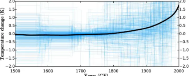
Figure 5 shows the individual Monte Carlo inversions to-gether with their average. We believe our results are con-sistent because similar mean North American GST histo-ries were obtained from different parametrizations (see Ap-pendix A). However, individual inversions in Fig. 5 exhibit a wide variability due to the large range of latitudes (∼80 to ∼18◦N) in the dataset of GST reconstructions.
Nevertheless, a clear warming transition is observed from the preindustrial era (1500–1800) to the postindustrial era (1800–2000). The temperature difference between the prein-dustrial mean (1500–1700) and the mean between the years (1961–1990) is 1.1 K. Because of the marked warming of the past 50 years, the total change of the average GST is 1.8 K between preindustrial time and the year 2000.
Figure 5.Mean North American GST change (black). Shown in blue are the 510 GST reconstructions inferred from the Monte Carlo inversion.
1500 1600 1700Years 1800 1900 2000 (CE)
1.5 1.5
1.0 1.0
0.5 0.5
0.0 0.0
0.5 0.5
1.0 1.0
1.5 1.5
2.0 2.0
Te
mp
era
tu
re
(
K
)
wr
t
1904
−
1980
Tree rings (Trouet et. al., 2013)
CRUTEM4 NAmGSTH (300 m)Pollen (Trouet et. al., 2013) Pollen (Viau et. al., 2006)Pollen (Viau et. al., 2012)
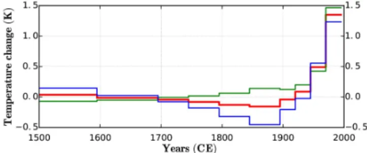
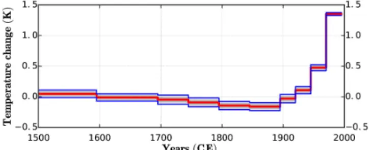
Figure 6.Mean North American GST history (blue) and maximum temperature range of accepted models (∼0.44 K) obtained from the Monte Carlo method (blue shade). Also shown are proxy-based SAT reconstructions for North America from 1500 to 2000 CE. All anomalies are displayed as departures from the 1904–1980 mean.
(2004). For instance, while a significant part of boreholes are located in higher latitudes (eastern and central Canada), tree-ring data are mainly obtained in lower latitudes (western US). Therefore, the spatial distribution of proxies could explain colder temperatures. Other possible reasons for those differ-ences are the seasonal bias of the proxies and the limitation of borehole climatology in resolving short-term variability.
The Little Ice Age (LIA) is not resolved because the bore-holes were truncated at 300 m, which is too shallow to allow for a clear LIA signal in most of the borehole profiles as can be shown with synthetic models (Mareschal and Beltrami, 1992) and was confirmed in several studies (Guillou-Frottier et al., 1998; Chouinard et al., 2007; Pickler et al., 2016b). Some profiles, such as the Fox Mine shown in Fig. 2, may in-deed show the LIA cooling, but the majority of them do not. In addition, because the LIA signal may vary both in time and in amplitude between regions, a marked signal cannot be expected from averaging weak and inconsistent signals.
3.2 Regional averages
The PAGES NAm2k working group divided the North Amer-ican continent into seven subregions for paleoclimate studies (McKay, 2014). The distribution of boreholes between these
regions is extremely uneven as shown in Table 2, with only four regions appearing adequately sampled (central and east-ern Canada, midwesteast-ern US, Arctic, and Pacific northwest). Furthermore, the sampling in the Arctic and the Pacific north-west is very biased because all the boreholes are close to the coast (Fig. 4). For the three other regions, the sampling is insufficient to obtain robust climate trends.
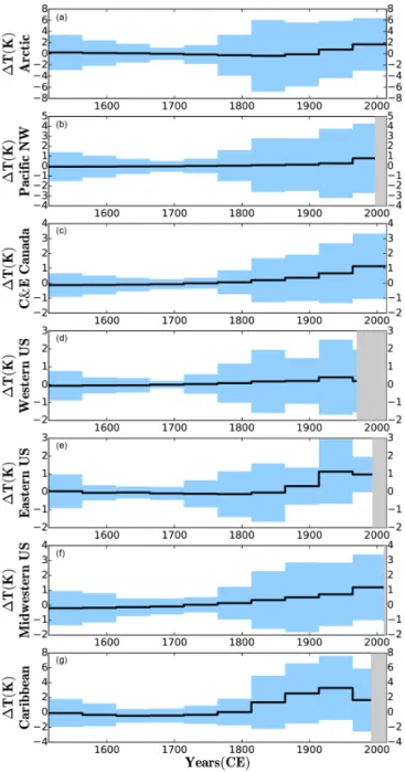
A warming by∼1.8 K for the past 200 years is observed in the Arctic (Fig. 7a), but the histories show wide variability. This variability suggests the need for smaller-scale regional analysis such as the pollen-based reconstructions of Gajew-ski (2015) and Viau and GajewGajew-ski (2009). Their findings il-lustrate that recent Arctic increases in temperature have ex-ceeded natural climate variability, which is consistent with borehole GST reconstructions.
The region of the Pacific northwest (western Canada and northwestern US) shows an increase in temperature of ∼0.8 K with a 95 % variability range of∼3.4 K for the last two centuries (Fig. 7b). This warming is consistent with pre-vious findings (Majorowicz and Safanda, 2001).
An average warming of ∼1.1 K with a 95 % variability range of∼2.2 K for the past two centuries is observed for central and eastern Canada (Fig. 7c), agreeing with previous studies (Beltrami et al., 1992; Guillou-Frottier et al., 1998).
The western US GST mean shows a small increase in tem-perature of∼0.2 K±1.8 K (Fig. 7d). This could be the result of strong irrigation processes and water flow at the sampling locations, but the number of borehole temperature profiles available in the region are insufficient to verify this. The lim-ited number of useful borehole temperature profiles for the western US (only nine) was logged in the 1960s, the most recent of which was measured in 1970. Thus, it is not pos-sible to reconstruct the past 40 years, when the increase in temperature recorded in weather stations was more marked.
The average reconstruction for the Midwestern US sug-gests a warming of∼1.3 K±2.0 K for the last 50-year aver-age (Fig. 7f). This recent warming has also been observed in previous GST reconstructions as well as SAT records (Skin-ner and Majorowicz, 1999) and could reflect the significant land use change in the region.
A warming of∼1.0 K±1.0 K has been reconstructed for the last 200 years in the eastern United States (Fig. 7e). How-ever, due to the rejection of borehole profiles affected by topography and water flow, the number of reconstructions made is too small to describe climate trends of the region with confidence.
Figure 7.Mean GST histories (black), the blue shaded areas repre-sent the 95 % confidence interval associated with the climate vari-ability of each area. Regional mean temperatures are shown until the year of measurement of the most recent thermal profile in each region.(a)Arctic (78 sites),(b)Pacific northwest (78 sites),(c) cen-tral and eastern Canada (220 sites),(d)western US (21 sites),(e)
eastern US (9 sites),(f)midwestern US (100 sites),(g)Caribbean (4 sites).
3.3 Geographical representation
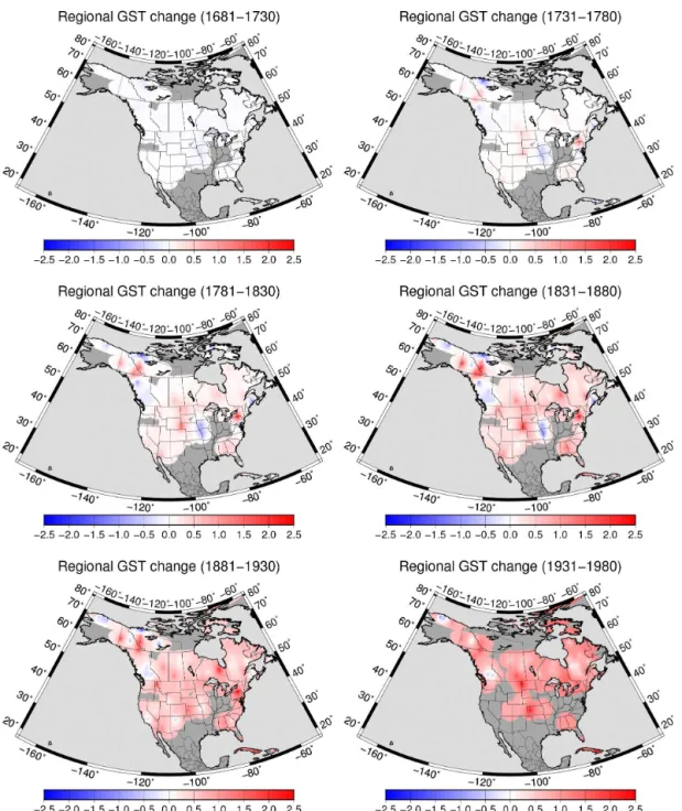
A North American regional analysis of GST changes is pre-sented as six geographical maps for different 50-year time intervals during the last 300 years (Fig. 8).
Trends prior to 1681 are not shown because they did not yield significant information. However, a small (∼0.5 K)
cooling is observed in certain regions. Previous small-scale regional analyses have reconstructed a LIA signal during this period (e.g., Beltrami and Mareschal, 1992; Chouinard et al., 2007). Furthermore, the regional variability of the cooling is consistent with previous studies, illustrating that not all re-gions of North America present a LIA signal (Gosselin and Mareschal, 2003b; Mann et al., 2009). However, due to the truncation at 300 m of the temperature–depth profiles ana-lyzed here, a clear LIA signal cannot be resolved.
Figure 8 indicates a warming trend of ∼1–2 K in most parts of North America during the last 200 years. This is consistent with previous studies (Huang et al., 2000; Harris and Chapman, 2001; Beltrami et al., 2003). A cooling trend is observed in central California. Stevens et al. (2008) show how this differs from the output of the ECHO-G model and postulates that it is the result of intensive irrigation in Cali-fornia’s central valley, which could drive a regional cooling signal (Kueppers et al., 2007). A similar cooling signal is ob-served in British Columbia which might be associated with irrigation in the Fraser Valley. On the Canadian east coast, Newfoundland presents little to no change with respect to the long-term mean. This agrees with meteorological data for the region (Gullett and Skinner, 1992). The absence of temperature profiles along the Gulf coast and Mexico does not allow for any determination of climate trends. The south-western US is also a region where the number of boreholes is not enough for reliable reconstructions. For these regions, a multi-proxy approach would be necessary to improve the reconstruction of regional past climate in regions with an in-sufficient number of borehole profiles.
4 Conclusions
The average North American GST change reconstructed from 510 boreholes deeper than 300 m suggests a warming of ∼1.8 K for the last 200 years. However, these temperatures exhibit a wide range of spatial variability among all regions. For instance, reconstructed regional GST changes for seven climate distinct regions, defined within the PAGES NAm2k project, suggest a warming range of∼0.5 to∼2.0 K with a standard deviation (?) no smaller than 0.5 K. Furthermore, regional variations in GST yield a warming range of 1 to 2 K between 1780 and 1980. These warming trends are consistent with multi-proxy reconstructions.
Figure 8.Spatial variability in the GST variation (in kelvin) from 1681 to 1980. Each panel shows a regionally interpolated mean GST over 50 years. The surface has been masked for zones without at least one datum within a radius of 400 km. Ground surface temperature changes are presented as departures from long-term mean surface temperatures prior to 1500 CE.
5 Data availability
The sources of all the data used in this study are listed in Table 1.
North American borehole temperature profiles valid for climate reconstructions were uploaded to Figshare (https:// figshare.com/s/0a1d213c3814024c4333) and published with doi:10.6084/m9.figshare.2062140.
Appendix A: Tests with different parametrizations
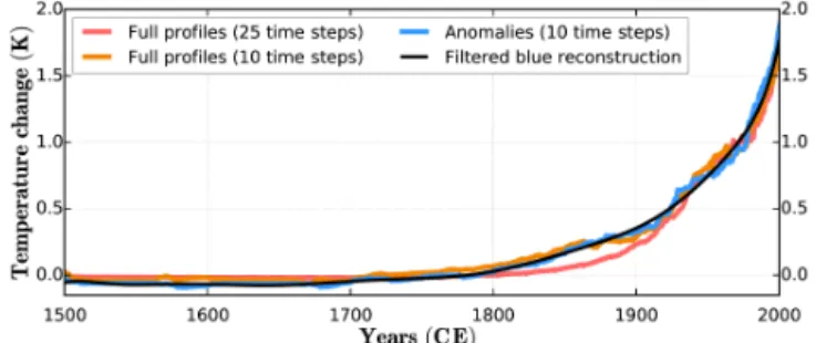
In this appendix, we have assessed the consistency of the re-sults obtained for several time parametrizations and different methods used to obtain the geothermal steady state. In bore-hole climatology, two distinct methods can be used to deter-mine the geothermal “quasi” steady state: (1) calculating lin-ear regression of the lowermost 100 m (Beltrami et al., 2011, 2015) and (2) including T0andŴ0into the parameter vec-tor and solving the system of equations using the full profile (Pickler et al., 2016a). The first method was utilized in this study. However, a validation test was run to ensure that both methods produced consistent results. The full profile method yielded mean temperatures similar to those calculated using the linear regression (Fig. A1). The main difference in the individual inversion consisted in a smaller deviation of the reconstructed temperatures and a smaller jump at the start of the GST history.
Another validation test was performed to ensure that the number and distribution of the time steps did not signifi-cantly affect the mean GSTs. Increasing the number of time steps from 10 to 25 in the inversion reconstructed similar mean temperature trends. Furthermore, an inversion utiliz-ing equal length time steps was compared with the ones pre-sented in the results, which use time steps of varying length. Both methods gave similar results.
These validation tests demonstrate the consistency of our results and the robustness of our reconstructions when utiliz-ing various parametrizations.
Acknowledgements. We acknowledge the work of many researchers in the last half century who have contributed data to the borehole climate community; these data are included in this work. This study was undertaken as part of the Past Global Changes (PAGES) project, which in turn received support from the US and Swiss national science foundations. Special thanks to William D. Gosnold for providing information about Midwestern boreholes and Jason E. Smerdon for suggesting this collaboration. This work was supported by grants from the Natural Sciences and Engineering Research Council of Canada Discovery grant (NSERC DG 140576948) and the Canada Research Program (CRC 230687) to H. Beltrami. Computational facilities were provided by the Atlantic Computational Excellence Network (ACEnet-Compute Canada) with support from the Canadian Foundation for Inno-vation. H. Beltrami holds a Canada Research Chair in Climate Dynamics. Fernando Jaume-Santero and Carolyne Pickler are funded by graduate fellowships from a NSERC-CREATE Training Program in Climate Sciences based at St. Francis Xavier University.
Edited by: M.-F. Loutre
Reviewed by: two anonymous referees
References
PAGES 2k Consortium, 2013: Continental-scale temperature vari-ability during the past two millennia, Nat. Geosci., 6, 339–346, 2013.
Bartlett, M. G., Chapman, D. S., and Harris, R. N.: Snow and the ground temperature record of climate change, J. Geophys. Res.-Earth, 109, F04008, doi:10.1029/2004JF000224, 2004. Bauer, S. E., Bausch, A., Nazarenko, L., Tsigaridis, K., Xu, B.,
Ed-wards, R., Bisiaux, M., and McConnell, J.: Historical and future black carbon deposition on the three ice caps: Ice core measure-ments and model simulations from 1850 to 2100, J. Geophys. Res.-Atmos., 118, 7948–7961, doi:10.1002/jgrd.50612, 2013. Beck, A. E.: Climatically perturbed temperature gradient and their
effect on regional and continental heat-flow means, Tectono-physics, 41, 17–39, 1977.
Beltrami, H. and Bourlon, E.: Ground warming patterns in the Northern Hemisphere during the last five centuries, Earth Planet. Sc. Lett., 227, 169–177, doi:10.1016/j.epsl.2004.09.014, 2004. Beltrami, H. and Mareschal, J.-C.: Ground temperature histories
for central and eastern Canada from geothermal measurements: Little Ice Age signature, Geophys. Res. Lett., 19, 689–692, doi:10.1029/92GL00671, 1992.
Beltrami, H., Jessop, A. M., and Mareschal, J.-C.: Ground tem-perature histories in eastern and central Canada from geother-mal measurements: evidence of climatic change, Global Planet. Change, 6, 167–183, doi:10.1016/0921-8181(92)90033-7, 1992. Beltrami, H., Gosselin, C., and Mareschal, J. C.: Ground surface temperatures in Canada: Spatial and temporal variability, Geo-phys. Res. Lett., 30, 1499, doi:10.1029/2003GL017144, 2003. Beltrami, H., Smerdon, J. E., Matharoo, G. S., and Nickerson, N.:
Impact of maximum borehole depths on inverted temperature histories in borehole paleoclimatology, Clim. Past, 7, 745–756, doi:10.5194/cp-7-745-2011, 2011.
Beltrami, H., Matharoo, G. S., and Smerdon, J. E.: Ground sur-face temperature and continental heat gain: uncertainties from
underground, Environ. Res. Lett., 10, 014009, doi:10.1088/1748-9326/10/1/014009, 2015.
Benfield, A. E.: Terrestrial heat flow in Great Britain, P. Roy. Soc. Lond. A, 173, 428–450, 1939.
Bodri, L. and Cermak, V.: Borehole Climatology, Elsevier, Amster-dam, 2007.
Briffa, K. R., Bartholin, T. S., Eckstein, D., Jones, P. D., Karlén, W., Schweingruber, F. H., and Zetterberg, P.: A 1,400-year tree-ring record of summer temperatures in Fennoscandia, Nature, 346, 434–439, doi:10.1038/346434a0, 1990.
Bullard, E. C.: Heat Flow in South Africa, P. Roy. Soc. Lond. A, 173, 474–502, 1939.
Carslaw, H. S. and Jaeger, J. C.: Conduction of Heat in Solids, Ox-ford Science Publications, New York, 1959.
Cermak, V.: Underground temperature and inferred climatic tem-perature of the past millenium, Palaeogeogr. Palaeocl., 10, 1–19, 1971.
Chouinard, C., Fortier, R., and Mareschal, J.-C.: Recent climate variations in the subarctic inferred from three borehole tempera-ture profiles in northern Quebec, Canada, Earth Planet. Sc. Lett., 263, 355–369, doi:10.1016/j.epsl.2007.09.017, 2007.
Clauser, C. and Mareschal, J.-C.: Ground temperature history in central Europe from borehole temperature data, Geophys. J. Int., 121, 805–817, doi:10.1111/j.1365-246X.1995.tb06440.x, 1995. Davis, B., Brewer, S., Stevenson, A., and Guiot, J.: The
tempera-ture of Europe during the Holocene reconstructed from pollen data, Quaternary Sci. Rev., 22, 1701–1716, doi:10.1016/S0277-3791(03)00173-2, 2003.
Douglass, A. E.: Climatic cycles and tree-growth, vol. 1, Carnegie Institution of Washington, 1919.
Gajewski, K.: Quantitative reconstruction of Holocene tempera-tures across the Canadian Arctic and Greenland, Global Planet. Change, 128, 14–23, doi:10.1016/j.gloplacha.2015.02.003, 2015.
García-García, A., Cuesta-Valero, F. J., Beltrami, H., and Smerdon, J. E.: Simulation of air and ground tempera-tures in PMIP3/CMIP5 last millennium simulations: implica-tions for climate reconstrucimplica-tions from borehole temperature profiles, Environ. Res. Lett., 11, 044022, doi:10.1088/1748-9326/11/4/044022, 2016.
George, S. S. and Ault, T. R.: The imprint of climate within Northern Hemisphere trees, Quaternary Sci. Rev., 89, 1–4, doi:10.1016/j.quascirev.2014.01.007, 2014.
González-Rouco, J. F., Beltrami, H., Zorita, E., and von Storch, H.: Simulation and inversion of borehole temperature profiles in sur-rogate climates: Spatial distribution and surface coupling, Geo-phys. Res. Lett., 33, l01703, doi:10.1029/2005GL024693, 2006. González-Rouco, J. F., Beltrami, H., Zorita, E., and Stevens, M. B.: Borehole climatology: a discussion based on contributions from climate modeling, Clim. Past, 5, 97–127, doi:10.5194/cp-5-97-2009, 2009.
Gosselin, C. and Mareschal, J.-C.: Variations in ground surface tem-perature histories in the Thompson Belt, Manitoba, Canada: en-vironment and climate changes, Global Planet. Change, 39, 271– 284, doi:10.1016/S0921-8181(03)00120-6, 2003a.
Guillou-Frottier, L., Mareschal, J.-C., and Musset, J.: Ground sur-face temperature history in central Canada inferred from 10 se-lected borehole temperature profiles, J. Geophys. Res.-Sol. Ea., 103, 7385–7397, doi:10.1029/98JB00021, 1998.
Gullett, D. W. and Skinner, W. R.: The state of Canada’s climate: temperature change in Canada 1895–1991, A State of Environ-ment Report, Ottawa, Supply and Services Canada, No. 92-2, SOE Report, p. 36, 1992.
Hansen, J., Ruedy, R., Sato, M., and Lo, K.: GLOBAL SUR-FACE TEMPERATURE CHANGE, Rev. Geophys., 48, rG4004, doi:10.1029/2010RG000345, 2010.
Hansen, J., Sato, M., Kharecha, P., and von Schuckmann, K.: Earth’s energy imbalance and implications, Atmos. Chem. Phys., 11, 13421-13449, doi:10.5194/acp-11-13421-2011, 2011. Harris, R. N. and Chapman, D. S.: Geothermics and climate
change: 2. Joint analysis of borehole temperature and mete-orological data, J. Geophys. Res.-Sol. Ea., 103, 7371–7383, doi:10.1029/97JB03296, 1998.
Harris, R. N. and Chapman, D. S.: Mid-latitude (30◦–60◦N) cli-matic warming inferred by combining borehole temperatures with surface air temperatures, Geophys. Res. Lett., 28, 747–750, doi:10.1029/2000GL012348, 2001.
Hotchkiss, W. O. and Ingersoll, L. R.: Post-glacial time calcula-tions from recent geothermal measurements in the Calumet Cop-per Mines, J. Geol., 42, 113–142, 1934.
Huang, S., Pollack, H., and Shen, P.: Global database of borehole temperatures and climate reconstructions, PAGES Newsletter, 7, 18–19, 1999.
Huang, S., Pollack, H. N., and Shen, P.-Y.: Temperature trends over the past five centuries reconstructed from borehole temperatures, Nature, 403, 756–758, doi:10.1038/35001556, 2000.
Jackson, D. D.: Interpretation of inaccurate, insufficient, and incon-sistent data, Geophys. J. Int., 28, 97–110, 1972.
Jacques, J.-M. S., Cumming, B. F., Sauchyn, D. J., and Smol, J. P.: The bias and signal attenuation present in conventional pollen-based climate reconstructions as assessed by early cli-mate data from Minnesota, USA, PloS One, 10, e0113806, doi:10.1371/journal.pone.0113806, 2015.
Jaume-Santero, F., Beltrami, H., and Mareschal, J.-C.: North Amer-ican borehole temperature profiles suitable for climate studies, doi:10.6084/m9.figshare.2062140, 2016.
Jaupart, C. and Mareschal, J.-C.: Heat generation and transport in the Earth, Cambridge University Press, 2011.
Jaupart, C. and Mareschal, J. C.: Heat flow and the structure of the lithosphere, in: Treatise on Geophysics, vol. 6, 2nd Edn., edited by: Watts, A. B., chap. 5, Elsevier, New York, 217–253, 2015. Jessop, A. M., Allen, V. S., Bentkowski, W., Burgess, M., Drury, M.,
Judge, A. S., Lewis, T., Majorowicz, J., Mareschal, J., and Tay-lor, A.: The Canadian geothermal data compilation, Tech. rep., Geological Survey of Canada, 2005.
Jones, P. D., Lister, D. H., Osborn, T. J., Harpham, C., Salmon, M., and Morice, C. P.: Hemispheric and large-scale land-surface air temperature variations: An extensive revision and an update to 2010, J. Geophys. Res.-Atmos., 117, d05127, doi:10.1029/2011JD017139, 2012.
Kueppers, L. M., Snyder, M. A., and Sloan, L. C.: Irrigation cooling effect: Regional climate forcing by land-use change, Geophys. Res. Lett., 34, l03703, doi:10.1029/2006GL028679, 2007.
Kukkonen, I. T. and Jõeleht, A.: Weichselian temperatures from geothermal heat flow data, J. Geophys. Res.-Sol. Ea., 108, 2163, doi:10.1029/2001JB001579, 2003.
Lachenbruch, A. H. and Marshall, B. V.: Changing climate: Geothermal evidence from permafrost in the Alaskan Arctic, Sci-ence, 234, 689–696, 1986.
Lanczos, C.: Linear Differential Operators, D. Van Nostrand, Princeton, N. J., 1961.
Lane, A. C.: Geotherms of Lake Superior Copper Country, Geol. Soc. Am. Bull., 34, 703–720, doi:10.1130/GSAB-34-703, 1923. Lewis, T.: Climate change inferred from underground temperatures,
Paleogeogr. Paleoclimatol., 98, 71–281, 1992.
Lewis, T. J. and Wang, K.: Geothermal evidence for defor-estation induced warming: Implications for the Climatic im-pact of land development, Geophys. Res. Lett., 25, 535–538, doi:10.1029/98GL00181, 1998.
Majorowicz, J. A. and Safanda, J.: Composite surface temperature history from simultaneous inversion of borehole temperatures in western Canadian plains, Global Planet. Change, 29, 231–239, doi:10.1016/S0921-8181(01)00092-3, 2001.
Mann, M. E., Zhang, Z., Hughes, M. K., Bradley, R. S., Miller, S. K., Rutherford, S., and Ni, F.: Proxy-based reconstructions of hemispheric and global surface temperature variations over the past two millennia, P. Natl. Acad. Sci. USA, 105, 13252–13257, 2008.
Mann, M. E., Zhang, Z., Rutherford, S., Bradley, R. S., Hughes, M. K., Shindell, D., Ammann, C., Faluvegi, G., and Ni, F.: Global Signatures and Dynamical Origins of the Little Ice Age and Medieval Climate Anomaly, Science, 326, 1256–1260, doi:10.1126/science.1177303, 2009.
Mareschal, J.-C. and Beltrami, H.: Evidence for recent warming from perturbed geothermal gradients: examples from eastern Canada, Clim. Dynam., 6, 135–143, doi:10.1007/BF00193525, 1992.
Mareschal, J.-C., Rolandone, F., and Bienfait, G.: Heat flow vari-ations in a deep borehole near Sept-Iles, Québec, Canada: Paleoclimatic interpretation and implications for regional heat flow estimates, Geophys. Res. Lett., 26, 2049–2052, doi:10.1029/1999GL900489, 1999.
Masson-Delmotte, V., Schulz, M., Abe-Ouchi, A., Beer, J., Ganopolski, A., González Rouco, J. F., Jansen, E., Lambeck, K., Luterbacher, J., Naish, T., Osborn, T., Otto-Bliesner, B., Quinn, T., Ramesh, R., Rojas, M., Shao, X., and Timmermann, A.: Infor-mation from Paleoclimate Archives. In: Climate Change 2013: The Physical Science Basis. Contribution of Working Group I to the Fifth Assessment Report of the Intergovernmental Panel on Climate Change, edited by: Stocker, T. F., Qin, D., Plattner, G.-K., Tignor, M., Allen, S. G.-K., Boschung, J., Nauels, A., Xia, Y., Bex, V., and Midgley, P. M., Cambridge University Press, Cam-bridge, United Kingdom and New York, NY, USA, 2013. McKay, N.: A novel multiproxy approach: The PAGES North
America 2k working group, PAGES magazine, 22, p. 100, http://www.pages-igbp.org/download/docs/magazine/2014-2/ PAGESmagazine_2014(2)_100_McKay.pdf (last access: 13 December 2016), 2014.
Morice, C. P., Kennedy, J. J., Rayner, N. A., and Jones, P. D.: Quantifying uncertainties in global and regional temperature change using an ensemble of observational estimates: The HadCRUT4 data set, J. Geophys. Res.-Atmos., 117, d08101, doi:10.1029/2011JD017187, 2012.
Mosegaard, K. and Tarantola, A.: Monte Carlo sampling of solu-tions to inverse problems, J. Geophys. Res.-Sol. Ea., 100, 12431– 12447, doi:10.1029/94JB03097, 1995.
Oeschger, H. and Langway, C. J.: The environmental record in glaciers and ice sheets, New York, NY (US), Wiley-Interscience, 1989.
PAGES 2k-PMIP3 group: Continental-scale temperature variabil-ity in PMIP3 simulations and PAGES 2k regional temperature reconstructions over the past millennium, Clim. Past, 11, 1673– 1699, doi:10.5194/cp-11-1673-2015, 2015.
Parker, R. L.: Understanding inverse theory,
Annu. Rev. Earth Planet. Sc., 5, 35–64,
doi:10.1146/annurev.ea.05.050177.000343, 1977.
Parker, R. L.: Geophysical inverse theory, Princeton university press, 1994.
Pickler, C., Beltrami, H., and Mareschal, J.-C.: Laurentide Ice Sheet basal temperatures during the last glacial cycle as inferred from borehole data, Clim. Past, 12, 115–127, doi:10.5194/cp-12-115-2016, 2016a.
Pickler, C., Beltrami, H., and Mareschal, J.-C.: Climate trends in northern Ontario and Quebec from borehole temperature profiles, Clim. Past Discuss., doi:10.5194/cp-2016-55, in review, 2016b. Pollack, H. N. and Smerdon, J. E.: Borehole climate
reconstruc-tions: Spatial structure and hemispheric averages, J. Geophy. Res.-Atmos., 109, d11106, doi:10.1029/2003JD004163, 2004. Putnam, S. N. and Chapman, D. S.: A geothermal climate change
observatory: First year results from Emigrant Pass in north-west Utah, J. Geophys. Res.-Sol. Ea., 101, 21877–21890, doi:10.1029/96JB01903, 1996.
Sass, J. H., Lachenbruch, A. H., and Jessop, A. M.: Uniform heat flow in a deep hole in the Canadian Shield and its pa-leoclimatic implications, J. Geophys. Res., 76, 8586–8596, doi:10.1029/JB076i035p08586, 1971.
Scattolini, R.: Heat flow and heat production studies in North Dakota, PhD thesis, University of North Dakota, 1978.
Shen, P. Y. and Beck, A. E.: Least squares inversion of borehole temperature measurements in functional space, J. Geophys. Res.-Sol. Ea., 96, 19965–19979, doi:10.1029/91JB01883, 1991. Skinner, W. R. and Majorowicz, J. A.: Regional climatic
warm-ing and associated twentieth century land-cover changes in north-western North America, Clim. Res., 12, 39–52, doi:10.3354/cr012039, 1999.
Smith, D. M., Allan, R. P., Coward, A. C., Eade, R., Hyder, P., Liu, C., Loeb, N. G., Palmer, M. D., Roberts, C. D., and Scaife, A. A.: Earth’s energy imbalance since 1960 in observa-tions and CMIP5 models, Geophys. Res. Lett., 42, 1205–1213, doi:10.1002/2014GL062669, 2015.
Stevens, M. B., González-Rouco, J. F., and Beltrami, H.: North American climate of the last millennium: Underground tem-peratures and model comparison, J. Geophys. Res.-Earth, 113, f01008, doi:10.1029/2006JF000705, 2008.
Tarantola, A. and Valette, B.: Generalized nonlinear inverse prob-lems solved using the least squares criterion, Rev. Geophys. Space Ge., 20, 219–232, 1982.
Thompson, L. G., Mosley-Thompson, E., Davis, M. E., Zagorod-nov, V. S., Howat, I. M., Mikhalenko, V. N., and Lin, P.-N.: Annually Resolved Ice Core Records of Tropical Climate Variability over the Past 1800 Years, Science, 340, 945–950, doi:10.1126/science.1234210, 2013.
Tikhonov, A. N. and Arsenin, V. Y.: Solutions of ill-posed problems, Wiley, New-York, 1977.
Trouet, V., Diaz, H. F., Wahl, E. R., Viau, A. E., Graham, R., Gra-ham, N., and Cook, E. R.: A 1500-year reconstruction of an-nual mean temperature for temperate North America on decadal-to-multidecadal time scales, Environ. Res. Lett., 8, 024008, doi:10.1088/1748-9326/8/2/024008, 2013.
Vasseur, G., Bernard, P., de Meulebrouck, J. V., Kast, Y., and Jolivet, J.: Holocene paleotemperatures deduced from geothermal measurements, Palaeogeogr. Palaeocl., 43, 237–259, doi:10.1016/0031-0182(83)90013-5, 1983.
Viau, A. and Gajewski, K.: Reconstructing millennial-scale, re-gional paleoclimates of boreal Canada during the Holocene, J. Climate, 22, 316–330, doi:10.1175/2008JCLI2342.1, 2009. Viau, A., Ladd, M., and Gajewski, K.: The climate of
North America during the past 2000 years reconstructed from pollen data, Global Planet. Change, 84–85, 75–83, doi:10.1016/j.gloplacha.2011.09.010, 2012.
Viau, A. E., Gajewski, K., Sawada, M. C., and Fines, P.: Millennial-scale temperature variations in North America dur-ing the Holocene, J. Geophys. Res.-Atmos., 111, d09102, doi:10.1029/2005JD006031, 2006.