www.nonlin-processes-geophys.net/13/185/2006/ © Author(s) 2006. This work is licensed
under a Creative Commons License.
in Geophysics
Influence of stability on the flux-profile relationships for wind speed,
φ
m
, and temperature,
φ
h
, for the stable atmospheric boundary layer
C. Yag ¨ue1, S. Viana1, G. Maqueda2, and J. M. Redondo3
1Dpto. Geof´ısica y Meteorolog´ıa, Universidad Complutense de Madrid, Spain
2Dpto. Astrof´ısica y Ciencias de la Atm´osfera, Universidad Complutense de Madrid, Spain 3Dpto. F´ısica Aplicada, Universidad Polit´ecnica de Catalunya, Barcelona, Spain
Received: 1 August 2005 – Revised: 21 April 2006 – Accepted: 21 April 2006 – Published: 21 June 2006 Part of Special Issue “Turbulent transport in geosciences”
Abstract. Data from SABLES98 experimental campaign
have been used in order to study the influence of stability (from weak to strong stratification) on the flux-profile rela-tionships for momentum, φm, and heat, φh. Measurements
from 14 thermocouples and 3 sonic anemometers at three levels (5.8, 13.5 and 32 m) for the period from 10 to 28 September 1998 were analysed using the framework of the local-scaling approach (Nieuwstadt, 1984a; 1984b), which can be interpreted as an extension of the Monin-Obukhov similarity theory (Obukhov, 1946). The results show increas-ing values ofφm andφhwith increasing stability parameter
ζ=z/3, up to a value ofζ≈1–2, above which the values re-main constant. As a consequence of this levelling off inφm
andφhfor strong stability, the turbulent mixing is
underesti-mated when linear similarity functions (Businger et al., 1971) are used to calculate surface fluxes of momentum and heat. On the other hand whenφm andφh are related to the
gra-dient Richardson number,Ri, a different behaviour is found, which could indicate that the transfer of momentum is greater than that of heat for highRi. The range of validity of these linear functions is discussed in terms of the physical aspects of turbulent intermittent mixing.
1 Introduction
Turbulent transfer is one of the most important processes in geophysical flows, which is characterized by a high degree of nonlinearity (Redondo et al., 1996). For the atmosphere, this turbulent transport takes place mainly in its lower part, near to the ground where important interactions occur: the Atmospheric or Planetary Boundary Layer (ABL or PBL). This ABL shows stratification which is often stable during the night in mid-latitude sites (Yag¨ue and Cano, 1994a) and
Correspondence to:C. Yag¨ue ([email protected])
can exist for prolonged periods during the months of winter darkness at polar places (King and Anderson, 1988; 1994; Yag¨ue and Redondo 1995). In these conditions surface in-versions are common and sometimes very strong, suppress-ing vertical turbulent mixsuppress-ing which can be very dangerous in polluted atmospheres (Morgan and Bornstein, 1977; Ja-cobson, 2002). Stable stratification can also lead to pollu-tion problems in the ocean (Rodriguez et al., 1995). Surface based inversions are developed not only over the ground but also over the ocean, due to warm air advection over colder water, producing a stable atmospheric boundary layer over the ocean (Lange et al., 2004).
The quantities most frequently used within the ABL, for atmospheric dispersion and forecasting models, are surface fluxes of momentum and heat. These surface fluxes are very important because of their strong influence on the mean pro-files in the lower atmosphere. Moreover, exchange coeffi-cients and boundary layer heights, which are needed as input for air pollution models, depend on the surface fluxes (Bel-jaars and Holtslag, 1991). In order to describe these fluxes (momentum and heat are the most common but the proce-dure can be extended to any particular property such as pol-lutants, humidity, etc), formulas for non-dimensional wind and temperature gradients (the so-called universal similarity functions) are used. These formulas result from the applica-tion of the Monin-Obukhov (M-O) similarity theory (1954) which is a suitable framework for presenting micrometeo-rological data, as well as for extrapolating and predicting certain micrometeorological information when direct mea-surements of turbulent fluxes are not available (Arya, 2001). The similarity functions for momentum, φm, and heat, φh,
-0.5 0.0 0.5 1.0 1.5 2.0
14 15 16 17 18 19 20 21
Ri
Night
z=5.8 m 0
2 4 6
14 15 16 17 18 19 20 21
V(m s
-1)
Night
z=5.8 m
0.0 0.2 0.4 0.6 0.8 1.0
14 15 16 17 18 19 20 21
TKE(m
2s -2)
Night
z=5.8 m -90
-45 0 45 90 135 180 225
14 15 16 17 18 19 20 21
Direction (degrees)
Night
z=10 m
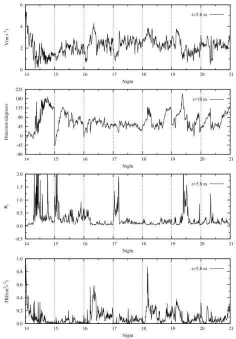
Fig. 1. Evolution of wind speed (5.8 m) and direction (10 m), Richardson number (5.8 m) and TKE (5.8 m) for the nights of the S-Period only.
mixing height (Berman et al., 1997). For unstable and neutral conditions good agreements between direct measurements and those evaluated from the similarity functions have been found (Businger et al., 1971; Hicks, 1976; H¨ogstr¨om, 1988; Sugita and Brutsaert, 1992). However under stable condi-tions the results are not so good, especially for weak winds where strong stratification takes place (Lee, 1997; Sharan et al., 2003). This difference between unstable and stable con-ditions is produced because turbulent fluxes are much larger for convective conditions than for stable ones (Cheng and Brutsaert, 2005).
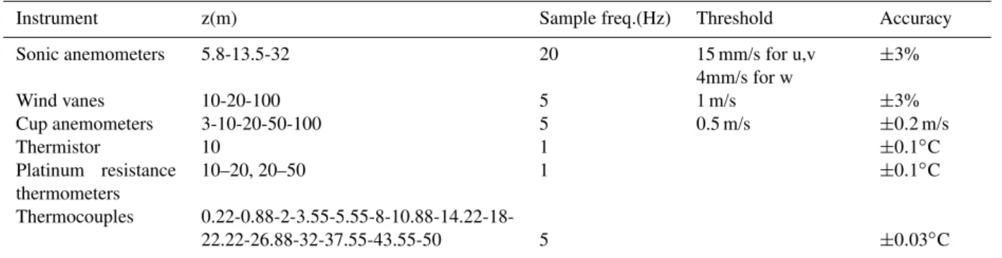
Table 1.Some of the instrumentation used at SABLES98 100 m tower.
Instrument z(m) Sample freq.(Hz) Threshold Accuracy
Sonic anemometers 5.8-13.5-32 20 15 mm/s for u,v 4mm/s for w
±3%
Wind vanes 10-20-100 5 1 m/s ±3%
Cup anemometers 3-10-20-50-100 5 0.5 m/s ±0.2 m/s
Thermistor 10 1 ±0.1◦C
Platinum resistance thermometers
10–20, 20–50 1 ±0.1◦C
Thermocouples
0.22-0.88-2-3.55-5.55-8-10.88-14.22-18-22.22-26.88-32-37.55-43.55-50 5 ±0.03◦C
currents, low level jets or perhaps mesoscale processes, while others associate intermittency with interactions be-tween turbulence and local mean gradients (Derbyshire, 1999). On the other hand, some authors (Zilitinkevich and Calanca, 2000; Zilitinkevich, 2002; Sodemann and Foken, 2004) have extended the theory of the atmospheric SBL by a distinction between nocturnal and long-lived stable boundary layers (winter polar regions). In the latter, the free atmosphere may influence the fluxes in the surface layer, and this would require a modification of the traditional M-O similarity theory which is taken into account by introducing the Brunt-V¨aisal¨a frequency in the similarity functions. Esau (2004) evaluated the non-local effect of the ambient atmospheric stratification on the parameterization of the surface drag coefficient, as the classical parameterization fails to estimate the turbulent exchange. We will estimate in-termittency from velocity probability distribution functions and structure function analysis as described in Mahjoub et al. (1998).
With all these considerations in mind, we have evalu-ated here the flux-profile relationships for a wide range of stability from SABLES98 data, analyzing the consequences of using some of the common functions to evaluate turbulent fluxes out of their range of validity. In the next section a brief description of the site where the experimental campaign took place and the instrumentation used will be given. In section 3 we present the methodology used to calculate the behaviour of φm andφh versus the local stability parameter z/3. In
Sect. 4 the main results of the study are presented and in Sect. 5 we discuss the mixing processes and intermittency related to the stability conditions and the turbulent Prandtl number. Finally the conclusions are presented relating our results to previous work in the ABL and laboratory and numerical experiments.
2 Site and measurements
The data used in this study is part of the SABLES98 (Sta-ble Atmospheric Boundary Layer Experiment in Spain) field campaign which took place in September 1998 (from 10 to 28) at the Research Centre for the Lower Atmosphere (CIBA), situated at 840 m above sea level on the Northern Spanish Plateau. The surrounding terrain is fairly flat and homogeneous. The Duero River flows along the SE bor-der of the plateau; two small river valleys, which may act as drainage channels in stable conditions, extend from the lower SW region. The place is surrounded by mountain ranges approximately 100 km distant extending from the SE to the North. Katabatic flows may be generated in the air flow over the mountainous terrain (Cuxart et al., 2000). In the present study we have concentrated on the so-called S-period (Stable S-period) comprising seven consecutive nights (from 18:00 GMT to 06:00 GMT) ranging from the night from 14 to 15 September to that from 20 to 21 September. The synoptic conditions were controlled by a High pressure system which produced light winds mainly from the NE-E direction.
Different instruments (3 sonic and 5 cup anemometers, 14 thermocouples, 3 wind vanes, etc) were deployed on a 100 m high tower. A summary of technical specifications and the heights at which these instruments were installed are given in Table 1. For further information on SABLES98 Cuxart et al. (2000) should be consulted. Five-minute means have been used to evaluate all the parameters in this study, which were provided (and calibrated) by the Risoe National Laboratory.
levels of turbulence. Periods with higher stability, which cor-responds to higher values of the Richardson number, low tur-bulent kinetic energy (TKE), and low surface winds, can be found for the nights of 14–15, 15–16, beginning of 17–18 and 20–21 September. The average wind direction is East, ranging from N to SE, and might be attributed mainly to local and orographic effects, most likely to drainage flows. How-ever, when different evolutions are analysed in detail, the in-teraction of turbulence and waves can be present and some stable records are sometimes interrupted by peaks of TKE. Such peaks could be produced by the breaking of internal gravity waves, which can generate strong local turbulence and increase the intermittency. These arguments are further explained below, see also Redondo et al. (1996), Yag¨ue et al. (2004).
3 Methodology
This study has been developed in the framework of the local-scaling approach, which can be interpreted as an extension of the M-O similarity to the stable boundary layer (Nieuw-stadt, 1984a, 1984b; Forrer and Rotach, 1997; Howell and Sun, 1999) when turbulent and stability local values are used instead of surface values.
Turbulent fluxes of momentum (τ) and heat (H) can be calculated directly from eddy correlation measurements or from velocity (u∗)and temperature scales (θ∗):
τ=−ρu′w′=ρu2
∗ (1)
H=ρcpw′θ′=−ρcpu∗θ∗ (2)
whereρ is the density andcp the specific heat for constant pressure. The covariancesu′w′andθ′w′ are directly
evalu-ated from the sonic anemometer measurements.
The similarity functions (φmandφh)for momentum and
heat are defined as non-dimensional forms of the mean wind speed and potential temperature gradients:
φm(ζ )=
kz u∗
∂u
∂z (3)
φh(ζ )=
kz θ∗
∂θ
∂z (4)
whereuandθare mean wind speed and potential tempera-ture, respectively,k the von Karman constant, zheight,u∗
friction velocity (related to turbulent momentum flux) and
θ∗ the scale temperature (related to turbulent heat flux) as
mentioned above. ζ=z/Lis a stability parameter defined as the ratio of height,z, to a length scaleLknown as Monin-Obukhov length:
L= −u
3
∗ k(g/T0)(H0/ρcp)
(5)
withT0 a reference temperature (near the surface), H0 the
surface heat flux andg the acceleration due to gravity. L
is a measure of the height of the dynamical influence layer where surface properties are transmitted (z<L). For z>L
the thermal influence is the dominant factor.
By using local-scaling, dimensional combinations of vari-ables measured at the same height can be expressed as a func-tion of a single independent parameter, z/3. The scale3is evaluated from Eq. (5) but replacing the surfaceu∗ by the
local friction velocity, and H0 by the local heat flux. 3is
generally dependent on height, while L is constant in the surface layer, so that3(0)=L. Similarly,φm andφhcan be
evaluated from local values ofu∗,θ∗ and local gradients of
wind speed and potential temperature. This has been the pro-cedure in this study. All the parameters have been calculated using the local values at each corresponding height (the 3 lev-els of the sonic anemometers, 5.8 m, 13.5 m and 32 m.). For the purpose of simplicity z/3has been denoted asζ. The M-O relationships become local-scaling if the heat flux and stress at level zare significantly different from the surface values. When the instruments at level zare in the surface layer, the M-O surface-layer scaling and local scaling are ap-proximately the same; if not, the fluxes at that level are lower than at the surface and M-O similarity does not apply (Klipp and Mahrt, 2004). In our study, where moderate to high sta-bility often appears, the surface layer can be below the 3 lev-els used. Normally the covariancev′w′is quite small when
the reference system of coordinates takesuas the wind in the mean direction, andv perpendicular to it, but for complete-ness it is used when available, and then the friction velocity, u∗, is evaluated as:
u∗= h
(−u′w′)2+(−v′w′)2i1/4 (6)
The temperature scale,θ∗, can be directly evaluated from: θ∗=
"
w′θ′
−u∗ #
(7)
When the covariances (u′w′,v′w′ andθ′w′) are not
avail-able, then turbulent fluxes of momentum and heat can be es-timated fromu∗ andθ∗, which are evaluated from standard
vertical profiles of mean values of wind speed and potential temperature using Eq. (3) and (4) once the functionsφm(ζ )
andφh(ζ )are known. In this case,ζ is also estimated from
standard mean values of temperature and wind through the gradient Richardson number:
Ri=
g θ0
∂θ ∂z
∂u ∂z
2 (8)
Using forms (3), (4) and (8), a relationship betweenζ andRi is directly found as:
Ri=ζ φh(ζ )
φ2
m(ζ )
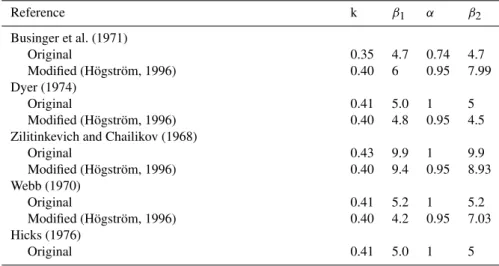
Table 2.Original functionsφm=1+β1ζandφh=α+β2ζfor different authors in stable conditions, and their modified forms (H¨ogstr¨om, 1996)
considering a value ofk=0.4 (von Karman constant)
Reference k β1 α β2
Businger et al. (1971)
Original 0.35 4.7 0.74 4.7 Modified (H¨ogstr¨om, 1996) 0.40 6 0.95 7.99 Dyer (1974)
Original 0.41 5.0 1 5
Modified (H¨ogstr¨om, 1996) 0.40 4.8 0.95 4.5 Zilitinkevich and Chailikov (1968)
Original 0.43 9.9 1 9.9
Modified (H¨ogstr¨om, 1996) 0.40 9.4 0.95 8.93 Webb (1970)
Original 0.41 5.2 1 5.2
Modified (H¨ogstr¨om, 1996) 0.40 4.2 0.95 7.03 Hicks (1976)
Original 0.41 5.0 1 5
which will be discussed in Sects. 4 and 5.
For each 5-min block of data,u(z) andθ(z) profiles were obtained from fitting a log-linear curve to the data:
u=az+blnz+c
θ=a′z+b′lnz+c′ (10)
The correlation coefficient of these fits was generally very high (>0.98), and only for some near-neutral conditions with strong winds the goodness of the fit for potential temperature decreased; in this case, fits with a correlation coefficient less than 0.9 have been excluded. Nieuwstadt (1984b) showed that the log-linear profile is the accepted profile in the sta-ble surface layer and King (1990), Yag¨ue and Cano (1994a), Forrer and Rotach (1997), and Cuxart et al. (2000) used them subsequently. Ifφmandφhare integrated overz, a log-linear
profile ofuandθis obtained.
From these fits, the gradient of wind speed and potential temperature are directly obtained for each level of interest as:
∂u
∂z=a+
b z ∂θ ∂z=a
′
+b
′
z
(11)
The levels used to obtain the fits were: 3.0, 5.8, 10.0, 13.5, 20, 32 and 50 m (for wind speed), and 0.88, 3.55, 5.55, 8, 10.88, 14.22, 18, 22.22, 26.88, 32, 37.55, y 43.55 m (for tem-perature).
Then vertical gradients were evaluated for the heights of interest, 5.8 m, 13.5 m and 32 m. With these gradients and
u∗andθ∗evaluated from Eqs. (6) and (7),φmandφhwere
directly obtained for the three heights using Eqs. (3) and (4). Functional forms for φm and φh were then obtained for a
wide range of stabilities (0<ζ <50) and compared with those widely used in the literature (Table 2 shows some of these
universal functions). H¨ogstr¨om (1988; 1996) revised some of these linear relations ofφm(ζ )andφh(ζ )for different values
of von Karman constant(k), establishing the slopes of the different relationships fork=0.40, which is widely accepted. Beljaars and Holtslag (1991) proposed a nonlinear formu-lation ofφm(ζ )andφh(ζ )which has recently been used in
some numerical studies (Basu, 2004). Handorf et al. (1999) confirmed the linear relations of the universal functions in the framework of the surface-layer and local-scaling forζ <0.8– 1 using the FINTUREX94 data. They mention that measure-ments in the range ofζ >2 cannot be found in the literature, since the SBL is not often that stable and the results are statis-tically uncertain; this underlines the importance of this kind of studies, it is precisely in strongly stratified situations when vertical mixing is inhibited and intermittency is strongest.
4 Results
In this section we summarize the results obtained grouped in four subsections. First of all the influence of local stability (ζ=z/3) on the non-dimensional gradient of wind speed,φm,
will be analyzed. Subsequently the behaviour of the non-dimensional gradient of potential temperature, φh, will be
studied, following with the relationship between the two sta-bility parameters, the gradient Richardson number and ζ, which are frequently used in the micrometeorological liter-ature (Launiainen, 1995). Finally the relationships between
φm,φhand the gradient Richardson number will be shown.
10−2 10−1 100 101 102 10−1
100 101 102 103
ζ φm
SABLES 98 Businger et al. (1971) Businger modified (Högström, 1996) Webb (1970)
(a)
10−2 10−1 100 101 102
10−1 100 101 102 103
ζ φm
SABLES 98 Businger et al. (1971) Businger modified (Högström, 1996) Webb (1970)
(b)
10−2 10−1 100 101 102
10−1 100 101 102 103
ζ φm
SABLES 98 Businger et al. (1971) Businger modified (Högström, 1996) Webb (1970)
(c)
Fig. 2.φmversus stability parameter for all the values calculated (S-period) at :(a)5.8 m,(b)13.5 m and(c)32 m. Functions found by other authors are shown for comparison.
otherwise, these intervals are: (<0.05), (0.05–0.1), (0.1–0.2), (0.2–0.3), (0.3–0.4), (0.4–0.5), (0.5–0.7), (0.7–1), (1–1.5), (1.5–2), (2–3), (3–4.5), (4.5–7), (7–10), (10–15), (15–20), (20–30), (>30). The criterion of Mahrt (1999) was adopted to establish different degrees of stability: weak stability for
ζ≤0.1, moderate stability for 0.1<ζ ≤1 and strong stability
forζ >1. The value ofζ to distinguish between weak and
moderate stability is obtained locating the maximum of the downward heat flux in stable conditions. While Mahrt ob-tained 0.06 atz=10 m, Grachev et al. (2005) showed that it depends onz, obtaining z/3≈0.02 forz=2 m., and z/3≈0.1 forz=5 and 14 m. Considering the range of possible values, we chose an approximation ofζ=0.1 as our criterion. 4.1 Flux-profile relationship for wind speed (φm)
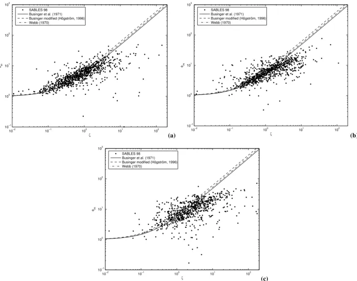
The relationship betweenφmandζ for all the data analyzed
for the S-period of SABLES98 can be seen in Fig. 2 for the
three heights studied (5.8 m, 13.5 m and 32 m). Businger et al. (1971) – original and modified by H¨ogstr¨om (1988)- and Webb (1970) have been drawn for comparison because these are probably the most widely used in the literature. If all the linear functions showed in Table 2 would have been drawn, no important differences would have been found. The data are more scattered as the height is increased, especially at 32 m in Fig. 2c where the points are less grouped around Businger’s and Webb’s lines.
As stability (ζ) increases, intermittent turbulence is more frequent, fluxes are decoupled from the surface values (Yag¨ue and Redondo, 1995), and the phenomenon ofz-less stratification (Nieuwstadt, 1984a; 1984b) is present:ζ is not controlling the momentum flux and φm tends to level off.
10−2 10−1 100 101 102 10−1
100 101 102 103
ζ φm
9 33
85 74 81 51
92 94
117 56 6841 28
18
10 13 SABLES 98
Businger et al. (1971) Businger modified (Högström, 1996) Webb (1970)
(a) 10
−2 10−1 100 101 102
10−1 100 101 102 103
ζ φm
15 30 53 50
53 8594
100
72 84 82 61 31 19
12 SABLES 98
Businger et al. (1971) Businger modified (Högström, 1996) Webb (1970)
(b)
10−2 10−1 100 101 102
10−1 100 101 102 103
ζ φm
13
1928 9 45 64 103
53 98 103 71
48 27
21 21
22 SABLES 98
Businger et al. (1971) Businger modified (Högström, 1996) Webb (1970)
(c)
Fig. 3.φmversus stability parameter grouped into intervals for the S-Period, at:(a)5.8 m,(b)13.5 m and(c)32 m. Functions found by other
authors are shown for comparison. Error bars indicate the standard deviation of the individual results contributing to the mean value in each stability bin. The number of samples in each stability bin is given over the upper bar or below it.
of turbulence. When this length scale becomes much smaller than the height above surface,z, turbulence no longer feels the presence of the ground and as a consequence an explicit dependence onzdisappears. The length scale of turbulence is proportional to 3 and in terms of local scaling this re-sult means that dimensionless quantities approach a constant value for large z/3. Then when stability is high (for large values of z/3) it is logical to think that there is a decoupling from the surface at relatively short heights (and these heights are probably over the surface layer).
The scaling and the onset ofz-less stratification are bet-ter seen if the data are grouped in inbet-tervals listed in section 4 above (Fig. 3). Where intervals contained too few sam-ples, the data groups were combined: the first interval for
z=13.5 m isζ <0.1, and forz=32 m isζ <0.2; on the other hand the last interval forz=5.8 m and 13.5 m is ζ >15, and
forz=32 mζ >30. The best agreement between SABLES98 data and Businger’s functions is found forz=5.8 m, for weak to moderate stability. It is in this zone where error bars are shorter and Businger’s and Webb’s functions are within these bars. A possible reason for this behaviour is that z=5.8 m is the closest level to the ground and it is more probable to be inside the surface layer, which is the portion of the ABL where the M-O theory (leading to the flux-profile re-lationships) is fulfilled. H¨ogstr¨om (1988) found an indica-tion of the levelling off forφm in the range 0.5<ζ <1, but
with few data points and a large scatter. Howell and Sun (1999) found thatφmlevelled off forζ around 0.5 for
Table 3.Linear fits forφmagainstζ(mean values) forζ <2.aand
β1are the coefficients of the fit,1a and1β1are the errors in the
estimation of these coefficients, andRis the correlation coefficient.
Level a 1a β1 1β1 R
5.8 m 2.05 0.17 4.05 0.22 0.9883 13.5 m 2.69 0.2 3.17 0.25 0.9779 32 m 3.9 0.5 3.0 0.5 0.9078
Table 4.Linear fits ofφmatz=5.8 m from the whole data forζ <2.
Level a 1a β1 1β1 R
5.8 m 2.17 0.14 3.96 0.17 0.6537
a large scatter, whereas atz=1.7 m that tendency could not be indicated due to the missing measurements. Cheng and Brutsaert (2005) found for CASES99 data that the stability functions show a linear behaviour up to a value ofζ=0.8, but for stronger stabilities both functions (φmandφh) approach
a constant with a value of approximately 7.
Another point to underline is that, for the three levels anal-ysed, the mean values of SABLES98 slightly overestimate the values given by Businger functions forζ approximately less than 1, and underestimate for ζ greater than 1. The value ofζ=1 corresponds toz=3, i.e. when the local M-O length (height of the dynamical influence layer) is equal to the height whereφmis evaluated (5.8 m, 13.5 m and 32 m).
The points to the left ofζ=1 (3>z) are within the layer of dynamical influence from the ground in each case but for the points to the right,z>3, decoupling from the surface is more likely, the intermittency increases, and a higher ten-dency to z-less stratification is found (Nieuwstadt, 1984a, 1984b). This is important to take into account when the flux-profiles relationships are used to calculate surface fluxes of momentum and heat in the stable atmospheric boundary layer. Most of times linear similarity functions are used (see Table 2), but for strong stability (light nocturnal winds) this can produce large errors in the estimation of the fluxes. Dif-ferent meteorological models used for dispersion studies or forecasting meteorological parameters make use of Businger et al. (1971) functions or other similar (Webb, 1970; Dyer, 1974) to obtain surface layer parameters asu∗,θ∗andL: u∗=
kz φm
∂u
∂z (12)
θ∗= kz φh
∂θ
∂z (13)
Ifφmandφhare overestimated (and this happens for strong
stability as it is shown in Fig. 3) thenu∗ andθ∗are
under-estimated and also the fluxes calculated from them. This
was pointed out by Louis (1979) using a weather forecast-ing model where Dyer’s similarity functions were used. As a consequence of having underestimated the surface fluxes of momentum and heat, the surface cooling could be several degrees below the observed values. Some climatic models (Noguer et al.,1998) have shown this problem for seasons and places where the atmospheric boundary layer is strongly stable.
A comparison of Fig. 3a (5.8 m) with Fig. 3c (32 m) shows that the lower level contains many more points withζ <0.1 than the upper level while the opposite is found for ζ >1 which would support the general idea of increasing stability with height.
A further point to note from Fig. 3 is that the mean val-ues of φm seem to be significantly greater than Businger
and Webb functions for the lowest intervals ofζ. However, this must be viewed in the context that this interval contains very few points (e.g. 9 points at 5.8 m). If a wider noctur-nal period is considered, namely the entire period from 10 to 26 September (see Fig. 4) where near-neutral stability is also included, the mean values for smallζ agree well with Businger′s and Webb′s functions, especially at the two lower heights (z=5.8 m in Fig. 4a and z=13.5 m in Fig. 4b). As it will be shown in the next subsection, this effect (even greater) is also apparent forφh. A possible explanation is related to
the few data found in the S-period for these low values of
ζ, which are not enough to obtain a significant statistic, and also to the influence of the global stability on the mixing pro-cesses; these few points are probably “contaminated” by a bulk stability and they are not truly near-neutral (as it was the case of the Businger and Webb datasets).
The general behaviour ofφmincreasing with stability
un-til a certain value of ζ approx. 1–2, followed by a level-ling off is in agreement with other relationships found in the literature for other locations (Forrer and Rotach, 1997; How-ell and Sun, 1999; Yag¨ue et al., 2001; Klipp and Mahrt, 2004; Cheng and Brutsaert, 2005), and would support the z-less theory, initially proposed by Wyngaard (1973) and extended by Nieuwstadt (1984a, 1984b).
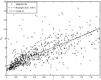
Finally, a specific similarity function of the formφm=a+
β1ζ was fitted to the mean values of SABLES98 data
10−2 10−1 100 101 102
10−1
100
101
102
103
ζ
φm
554 265
225 131
125 86
131 80
155 137
70
52 33
11 14 18
SABLES 98
Businger et al. (1971)
Businger modified (Högström, 1996)
Webb (1970)
(a) 10 −2
10−1 100 101 102
10−1
100
101
102
103
ζ
φm
257
163
155 163 109
119 145 238
12 23 35 70 111 111
95
SABLES 98
Businger et al. (1971)
Businger modified (Högström, 1996)
Webb (1970)
282
(b)
10−2 10−1 100 101 102
10−1
100
101
102
103
ζ
φm
157 154 251
142
93 46
119 161 128
124
129 87
17 52
35 55 82
SABLES 98
Businger et al. (1971)
Businger modified (Högström, 1996)
Webb (1970)
(c)
Fig. 4.As Fig. 3, but for the extended nocturnal period from 10 to 26 September.
similar to those obtained previously for the mean data, but the correlation coefficient is considerably lower.
It is also interesting to comment that Klipp and Mahrt (2004) found for CASES99 data that the correlation between φm and ζ for stable conditions is strongly
influ-enced by self-correlation. This self-correlation is evident for all values of ζ but is more significant for the largest values of stability, where the scatter of the data is large. They established that the reduction of φm below the
lin-ear prediction in strongly stable data could be due to self-correlation. Klipp and Mahrt (2004) proposed that if the gradient Richardson number is used as a stability parame-ter, these figures would suffer less from self-correlation; al-though there is also a self-correlation (vertical gradient of wind speed is the shared variable), it is much less compared to usingζ, due to the fact that the range of shear data is rel-atively small compared to turbulent fluxes, whereas it is the friction velocity which is the shared variable whenζ is used as stability parameter. An analysis of the similarity functions
versus gradient Richardson number will be shown below in Sect. 4.4.
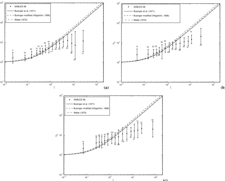
4.2 Flux-profile relationship for temperature (φh)
In this section, the dependence of the dimensionless gradi-ent of potgradi-ential temperature,φh, on the stability parameter is
discussed. As Fig. 7 shows, the results are much more scat-tered than those obtained forφmwhich could be attributed to several reasons: Duynkerke (1999) related this effect to the lower accuracy in the determination of the temperature gradients compared to those of wind speed. Another reason could be that the local gradient of potential temperature can be close to zero at lower stability, introducing larger errors in the evaluation ofφh. Handorf et al. (1999) showed large
values ofφhatz=4.2 m forζ <0.01, compared to those
pre-dicted by the linear functions, but no explanation was given. Yag¨ue et al. (2001) also found greater scatter for φh than
forφmusing Antarctic data, and large values ofφhfor
0 0.2 0.4 0.6 0.8 1 1.2 1.4 1.6 1.8 2 1
2 3 4 5 6 7 8 9 10 11
ζ φm
SABLES 98 Businger et al. (1971) Linear fit
(a) 0 0.2 0.4 0.6 0.8 1 1.2 1.4 1.6 1.8 2 1
2 3 4 5 6 7 8 9 10 11
ζ φm
SABLES 98 Businger et al. (1971) Linear fit
(b)
0 0.2 0.4 0.6 0.8 1 1.2 1.4 1.6 1.8 2 1
2 3 4 5 6 7 8 9 10 11
ζ φm
SABLES 98 Businger et al. (1971) Linear fit
(c)
Fig. 5.Linear fits ofφmmean values versusζfor stability parameter<2 at:(a)5.8 m,(b)13.5 m and(c)32 m. Businger et al. (1971) function is shown for comparison.
higher Richardson numbers was not due to undersampling. The scatter in both,φmandφh, may also be attributed to the
fact that turbulent scaling laws assume stationarity situations but the SBL is frequently non-stationary due to intermittent turbulence (Klipp and Mahrt, 2004). Zilitinkevich (2002) gives several features that may contribute to the scatter in the data, such as anisotropy of turbulent eddies under stable con-ditions and the possible effect of baroclinicity. Zilitinkevich and Esau there is little evidence(2003) show from LES data the influence of baroclinicity on turbulent fluxes in the SBL. Figure 7 shows the behaviour ofφhfor ζ intervals at the
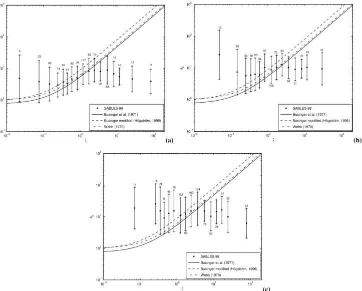
heights of 5.8 m, 13.5 m and 32 m. Due to the high stan-dard deviation, any comment about the relationship between
φhand stability seems less reliable than forφm. At z=5.8 m
there is reasonable agreement for 0.2≤ζ ≤2 but below that rangeφhis substantially larger than Businger and other
au-thors findings, although the statistics may not be reliable as
some intervals contain only a few points. As forφm,φhlevels
off for higher stability parameters,ζ >2. At the higher levels,
z=13.5 m and 32 m, there is little evidence of the similarity function following Businger’s or Webb’s functions. In fact, if a detailed analysis of the structure of the ABL is performed when highφhvalues are present with lowζ, a complex
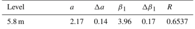
struc-ture of the lower atmosphere can be seen which is influenced by the presence of internal waves (Nai-Ping et al., 1983; Rees et al., 2000). These low values of ζ (for the S-period) are not truly neutral points and should not be used to do a fit in this range. If measurements from all nights, not just the S-period, are also included in the analysis, a much better agree-ment with Businger and Webb is found for low values ofζ
(Fig. 8). With regards to the levelling off ofφhfor greater
stability (ζ >1–2 approx.) the behaviour is similar to that of
φm, irrespective whether only the S-period is considered or
4.3 Relationship between the Richardson number and the stability parameter
The gradient Richardson number,Ri, which was defined in Eq. (8) is a widely used stability parameter relating thermal stratification to wind shear. Nieuwstadt (1984a) considered the relationship between the gradient Richardson number and the stability parameter,ζ, as another example of local-scaling, leading to a functional formRi=Ri (z/3) which is found with the definition ofφmandφh(Eq. 9). Fig. 9 shows
the behaviour of Ri for z=5.8 m, evaluated from Eq. (9) for each point of SABLES98 versus the stability parame-ter (in Fig. 9a) and then also averaged over the inparame-tervals of ζ(Fig. 9b). The results of the present study are consis-tent with the data shown by Nieuwstadt (1984a). The lines drawn for comparison correspond to Eq. (9) using Businger and Webb functions forφm andφh. These functions have
a horizontal asymptote for Ri≈0.2, which is a valid limit for turbulent transfer and which is derived from the values of the similarity functions found by Businger et al. (1971), H¨ogstr¨om (1996), and Webb (1970). Other studies (Kondo et al., 1978; Ueda et al., 1981) found a critical value for the flux Richardson number,Rf, of 0.143 and 0.1 respectively. ThisRf is related to the ratio of the eddy diffusivities and the gradient Richardson number, Rf=Ri Kh/Km. As will be discussed further below,Kh/Kmtends to decrease below 1 for high stability and then the criticalRf is less than the critical Ri, but if the stable boundary layer has continuous turbulence (Nieuwstadt data), then both critical numbers are approximately the same. In spite of our scattered results, the functions found by other studies (Webb, 1970; Businger et al., 1971; H¨ogstr¨om, 1996) are inside the error bars calcu-lated from SABLES98. As with the similarity functions, the dimensionless parameterRi, tends to a constant value in the limit of high values of z/3, which is again consistent with
z-less stratification.
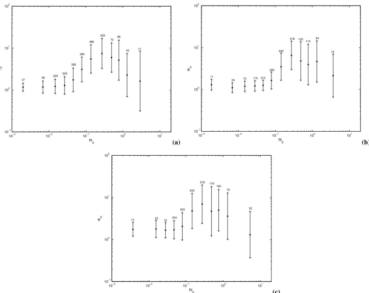
4.4 Relationship between similarity functions and gradient Richardson number.
As it was commented above, when relationships between turbulent and stability parameters are studied, one problem is self-correlation, i.e. the parameters share one or more variables. This feature was extensively explored by Klipp and Mahrt (2004) who concluded that the gradient Richard-son number, Ri, shows less self-correlation with the sim-ilarity functions, φm andφh, than the stability parameterz
3. Figure 10 and Fig. 11 show the dependence ofφm and
φh, respectively, onRi for the three levels analysed (5.8 m, 13.5 m and 32 m) for the whole period, not just the S-period, in order to have more points in a wide range of stability, considering that when Ri is used instead of z/3 the self-correlation is less.
For weaker stability, Ri<0.1, φm does not vary
signifi-cantly with stability whileφhhas a positive trend. The ratio
0 0.2 0.4 0.6 0.8 1 1.2 1.4 1.6 1.8 2 0
2 4 6 8 10 12 14 16
ζ φm
SABLES 98 Businger et al. (1971) Linear fit
Fig. 6.SABLES98 data and Linear fit ofφmversusζfor stability parameter<2 at 5.8 m. Businger et al. (1971) function is shown for comparison.
of the mean values in this stability range isφm/φh>1, which
decreases to approximately 1 asRi tends to 0.1. It can be easily deduced (Arya, 2001) that the ratio of the similarity functions,φm/φh, is equal to the ratio of the eddy
diffusiv-ities for heat and momentum,Kh/Km. Ifφm/φhdecreases
with stability, this would imply that the turbulent transfer of heat can be greater than that of momentum for near neutral stabilities.
The evolution for greater stabilities, Ri>0.1, shows that
φmtends to increase with stability and then levels off, or even
decreases for the greatest Richardson numbers, whileφh
in-creases to higher values thanφm and then levels off. This
evolution produces aφm/φh<1, which would be equivalent
to a greater turbulent transfer of momentum compared to the transfer of heat. This result, which is not shown when z/3
is used as stability parameter, is compatible with the results shown for winter Antarctic data in Yag¨ue et al. (2001), and has been related in previous works to the presence of internal gravity waves in the atmospheric boundary layer, and asso-ciated intermittent processes, usingKm andKh (Kondo et al., 1978; Wittich and Roth, 1984; Yag¨ue and Cano, 1994b). These waves can transfer momentum but much less heat, un-less they break.
5 Intermittency and mixing in the ABL
10−2 10−1 100 101 102 10−1
100 101 102 103
ζ φh
9 33
85 74
81 51
92 94 117
56 70
41 28
19 10
13 4
SABLES 98 Businger et al. (1971) Businger modified (Högström, 1996) Webb (1970)
(a) 10 −2
10−1 100 101 102
10−1 100 101 102 103
ζ φh
15
30
53 50 53 86
97
102 72 84
82 61
31 19 12
SABLES 98 Businger et al. (1971) Businger modified (Högström, 1996) Webb (1970)
(b)
10−2 10−1 100 101 102
10−1 100 101 102 103
ζ φh
14 18
28
8 46
65 102
53 100
104
73
50 28
24 22
21
SABLES 98 Businger et al. (1971) Businger modified (Högström, 1996) Webb (1970)
(c)
Fig. 7. φhversus stability parameter grouped into intervals for the S-Period, at:(a)5.8 m,(b)13.5 m and(c)32 m. Functions found by other authors are shown for comparison.
may be considered to produce a “wide tail in a skewed prob-ability density function (PDF)”. Kraichnan (1991) discusses further the spectral implications. In general an intermittent turbulent cascade will not exhibit a (-5/3) spectral energy cas-cade.
A detailed analysis of the turbulence at small scale may re-veal intermittent episodes in a stable atmosphere very clearly because of the high Kurtosis of the turbulent velocity PDFs. In this case, under stable stratification conditions, we are able to obtain a better quantification of the intermittency than in a convective situation. A practical way to calculate intermit-tency as a single parameter can be done following Mahjoub et al. (1998).
The velocity structure function is a basic tool to study the intermittent character of turbulence. The pth order velocity structure function is defined as
Sp(l)=(u(x+l)−u(x))p (14)
Velocity structure functions require the measurement of ve-locity at two different locations or times separated a distance
l(using Taylor’s hypothesis the correspondence between spa-tial and temporal increments is straightforward with the local mean velocity of the flow at the measured location). In fact, the use of this relation is limited to a low turbulence inten-sity. More information about the structure functions is given in Frisch (1995) but a small review of some basic ideas and developments in turbulence is at hand to interpret the mea-surements.
Following Kolmogorov’s theory (Kolmogorov, 1941), the self-similarity of the velocity structure function is attained in the inertial range, which is physically defined as a range of scales where both the forcing and the dissipation processes are irrelevant. For the K41 theory (Kolmogorov, 1941), the scaling exponent of the structure functions with separation
10−2 10−1 100 101 102 10−1
100 101 102 103
ζ φh
4 14 12 22 35 54 93 74 165 147 138 94 131 143 235
265 518
SABLES 98 Businger et al. (1971) Businger modified (Högström, 1996) Webb (1970)
(a) 10
−2
10−1 100 101 102
10−1 100 101 102 103
ζ
φh 266
249 235
144 115
109 161
166 158 111 111
94 70 35 24 SABLES 98
Businger et al. (1971) Businger modified (Högström, 1996) Webb (1970)
(b)
10−2 10−1 100 101 102
10−1 100 101 102 103
ζ φh
17 36
57 86 129 133 89 161 129 119 46 92 142
246 155 148
55 SABLES 98
Businger et al. (1971) Businger modified (Högström, 1996) Webb (1970)
(c)
Fig. 8.As Fig. 7, but for the extended nocturnal period from 10 to 26 September.
orderpof the statistical moment has been observed in many theoretical, experimental and numerical investigations (see Sreenivasan and Antonia (1997) for a review). In fact, this correction needed in K41 theory is referred to as intermit-tency, indicating that the average value of the energy dissi-pationεwill be different at different points in space (Frisch, 1995). The Extended Self Similarity (ESS) property, sug-gested by Benzi et al. (1993) is a very effective method to determine accurate scaling exponents. Moreover, the exis-tence of ESS could be used as a way to define an inertial range, even in situations where the phenomenological theory suggested by Kolmogorov (1941) and Kolmogorov (1962), known as K62, does not hold. This would apply to situations where there is a strong deviation from local homogeneity and isotropy, such as in the SBL flows (Babiano et al. 1997; Mahjoub et al., 1998). It is important to stress the point that neither K41 nor K62 are valid in non-homogeneous flows such as those in the ABL under strong stratification where
non-locality and non-homogeneity effects are indistinguish-able from intermittency.
Analysing the turbulence microscale at high sensor res-olutions, we can find intermittent episodes in a stable atmosphere. In this case, we are able to obtain a better quan-tification of the intermittency than in neutral or convective situations. The standard definition of intermittencyµ uses the sixth order structure function scaling exponentξ6:
µ=2−ξ6 (15)
which may be calculated as discussed in Mahjoub et al. (1998) or even in terms of the geometrical structure of the turbulent PDF zero crossings as:
ξp=
p
3+(3−D) (1−
p
3) (16)
where p is the order of the structure function, in this case
10−2 10−1 100 101 102 10−3
10−2 10−1 100 101 102
ζ
Ri
SABLES 98 Businger et al. (1971) Businger modified (Högström, 1996) Webb (1970)
(a)
10−2 10−1 100 101 102
10−3 10−2 10−1 100 101 102
ζ
Ri
9 33
85 74 81
5192 11756 70
41 28
10 13
7
19 SABLES 98
Businger et al. (1971) Businger modified (Högström, 1996) Webb (1970)
(b)
Fig. 9. Richardson number versusζ for the S-period at z=5.8 m: (a)All the individual SABLES98 data, (b)interval representation. Functions found by other authors are shown for comparison. Error bars indicate the standard deviation of the individual results contributing to the mean value in each stability bin. The number of samples in each stability bin is given over the upper bar or below it.
fourth order structure function, related to the Kurtosis or flat-ness, may also be used as a measure of intermittency. Fig-ure 12 compares the cumulative PDF’s of a strongly strati-fied situation in SABLES98 with a neutral one (error func-tion shape) normalized with their respective r.m.s turbulent fluctuations. Two 5 Hz wind speed series from an anemome-ter placed atz=20 m have been used. The deviations from the Gaussian cumulative PDF are also a direct measure of intermittency; clearly there is much more intermittency for the higher Richardson number situation (strongly stratified). There seems to exist a complex, non-linear relationship be-tween the intermittency, the fractal dimension and the mixing efficiency as discussed by Derbyshire and Redondo (1990).
Both the intermittency and the non-homogeneity produce changes in the spectral energy cascades, related to the second order structure functions, and these will produce strong vari-ations in the mixing efficiency. As a local indicator of the potential energy to kinetic energy ratio, we use the flux and gradient Richardson numbers,Rf andRi,parameters able to distinguish between different stratification types that also lead to different intermittencies. From the equation of the local turbulent kinetic energy (TKE), comparing buoyancy with the shear production term (the two first terms on the right-hand side):
∂T KE ∂t =−(u
′w′∂u
∂z+v
′w′∂v
∂z)+ g θ0
θ′w′−1
2
∂u′2
αw′
∂z −
1
ρ0
u′
α
∂p′
∂xα
−ε (17)
we obtain the Mixing efficiency or Flux Richardson number (in a reference frame withv=0):
Rf=
g θ0
w′θ′
u′w′∂u ∂z
(18)
Considering the following relationships between local fluxes and local gradients introduced first by Boussinesq (1877):
w′θ′=−K
h
∂θ
∂z (19)
u′w′=−K
m
∂u ∂z
we obtain that:
Rf=
Kh
Km
Ri (20)
with the gradient Richardson number as defined in (8). Considering also the Ozmidov scale and the integral length scale of the turbulence we can relate the Richardson numbers in a stratified fluid and their non-linear relationships to the measured universal functions.
The importance of measuring intermittency in internal wave breaking flow is that the use of structure functions and their difference may be used as a test for changes in the spec-trum of turbulence from 2-D to 3-D or from a local to a non-local situation. Experiments on irregular waves exhibit much more intermittency than in turbulence produced by regular ones (Mahjoub et al., 1998).
10−3 10−2 10−1 100 101
10−1
100
101
102
Rig
Φm
70 229 486
390
395
329 229 96 37
17 42 68
(a)
10−3 10−2 10−1 100 101
10−1
100
101
102
Rig
Φm 11
155 578
622
282 315 175 75 20
19 64 110
(b)
10−3
10−2
10−1
100
101 10−1
100 101 102
Rig
Φm
12 23 76 204
303
642 75 160 579
52 176
(c)
Fig. 10. φmversus gradient Richardson number for the extended nocturnal period from 10 to 26 September grouping in intervals for all
stability range at:(a)5.8 m,(b)13.5 m and(c)32 m. Error bars indicate the standard deviation of the individual results contributing to the mean value in each stability bin. The number of samples in each stability bin is given over the upper bar.
changes as a function of the integral length scale of the tur-bulence as a result of both non-homogeneity in space and anisotropy in different directions producing an anomalous distribution of also the most frequent and smallest fluctua-tions, and not only of the energetic but rare events, as is the case with the traditional intermittency. In non-homogeneous transfer dynamics, this balance includes both energy trans-fers from both, larger to smaller scales (normal cascade), and the anomalous energy transfers from smaller to larger scales (inverse cascade). In addition, the true scale-by-scale energy flux is also related to both, the transverse velocity structure and the work of pressure field.
There will be a mixing regime that is different depending on the local stability as it was commented above. The strong turbulent activity can be enough to penetrate the inversion layer and practically destroy it. In the limit of strong turbu-lence, the Reynolds analogy would apply and the turbulent
Prandtl number would tend to unity. But, in other cases the momentum and temperature (or mass) vertical transport may be very different (Carrillo et al., 2001).
It is clear that the transfer of heat and momentum, as well as the TKE, are well controlled by the gradient Richardson number. For very stable ranges, the coefficients are almost of the order of 1/1000. It is also interesting thatKh/Km<1 for strong stability. This is an indication of internal-gravity waves activity which can produce transfer of momentum but little transfer of heat if these waves do not break. The local turbulent parameters are also highly dependent on the friction velocity and on the inversion strength.
10−3
10−2
10−1
100
101 10−1
100 101 102
Rig
Φh
21 81
389 393 212 323
44 55 174
443
17 35
(a) 10−3
10−2
10−1
100
101 10−1
100 101 102
Rig
Φh
40
72 109 519
601
269 288 148 43
(b)
10−3 10−2 10−1 100 101
10−1 100 101 102
Rig
Φh
140 461
572
237
148 55
24
83 120
(c)
Fig. 11.As Figure 10, but forφh.
atmospheric data. The functional relationships are not con-clusive due to the difficulty in the calculation of higher or-der moments but intermittency clearly increases with higher stability. The effect of stratification on the inverse turbulent Prandtl number, which is a dimensionless number defined as the ratio of the eddy diffusivity for heat to momentum
Kh/Km has been studied in many laboratory experiments, and this number decreases as stability (Richardson number) increases for strong stratifications, showing the difference between the turbulent mixing of momentum and heat. Some-times this difference is ignored for simplicity but this leads to an underestimation of turbulent momentum transport at stable conditions. The observed behaviour supports the idea that under strong stable conditions (marked by high Richard-son number, even greater than the critical 0.25) mixing of heat is inhibited to a greater extent compared to that of mo-mentum. The role of internal gravity waves in this situation of intermittent and sporadic turbulence seems responsible for the more efficient transfer of momentum.
6 Summary and conclusions
The influence of local stability, as measured by the stabil-ity parameter ζ=z/3and the gradient Richardson number, on the non-dimensional gradients of wind speed and temper-ature,φmandφh, respectively, has been studied using data
from the experiment SABLES98 for a wide range of stabil-ity (from weak to strong). When no direct measurements (from sonic anemometers) are available, the universal sim-ilarity functions φm andφh for non-dimensional wind and
for strong stability has been analysed, and the influence of in-termittency on this very stable regime has been discussed. A number of conclusions can be drawn from the present work: 1. The general behaviour (though with greater scatter for
φh) obtained in the relationships between the
similar-ity functions, φm andφh, and z/3 is an increase with
stability up to a certain value (ζ >1–2approx.),above whichφmandφhtend to level off, staying almost
con-stant for greater stabilities. For these higher stabilities, the differences between SABLES98 data and Businger et al. (1971) functions become substantial. The best agreement is found at the lowest level (z=5.8 m) which could be related to the reduced intermittency closer to the ground.
2. A linear fit ofφmversus z/3to SABLES98 data for the
three heights considered (5.8 m, 13.5 m and 32 m) and
forζ <2, showed a decreasing slope with height. This
result supports the importance of using local-scaling even when stability is weak to moderate.
3. For weak stability, ζ <0.1, φh showed unexpectedly
large values for the S-period, especially at the higher levels which could be related to the interaction of tur-bulence with internal waves. This interaction results in rapid local mixing and would give low values ofζ even in an overall context of stable stratification, as it is the case for this S-period. When many near-neutral data are introduced in the analysis, this phenomenon is masked by averaging with lower values forφhobtained from the
lower stability periods.
4. The use of the common linear similarity functions for
ζ >1 can produce overestimation of the φm and φh
values and a corresponding underestimation of the sur-face fluxes. Such an error in their estimates would af-fect the reliability of atmospheric circulation models and dispersion models where this information is used to evaluate the turbulent fluxes and other parameters. 5. The relationships between φm, φh and the gradient
Richardson number have also been studied. Some au-thors (Klipp and Mahrt, 2004) have pointed out that self-correlation between the similarity functions and the gradient Richardson number,Ri, would be much less of an issue than between the similarity functions and the stability parameter,ζ. SABLES98 results revealed differences in the behaviour ofφmversusRi compared to that ofφh, which provides insight in the relative
mag-nitude of momentum transfer to heat transfer. For high stabilities it was found thatφm/φhis less than 1, which
would be equivalent to a greater transfer of momentum compared to the transfer of heat, which can also be re-lated to the nonlinear Prandtl number. This change in the ratio could be related to the presence of internal-gravity waves and resulting intermittency in the SBL.
−3 −2 −1 0 1 2 3
0 0.1 0.2 0.3 0.4 0.5 0.6 0.7 0.8 0.9 1
Normalized (v−<v>/rms)
Normalized Data Points
Strongly stratified Neutral
Fig. 12. Comparison of the cumulative normalized PDF of a neu-tral situation (dashed line) with low Richardson number and of a strongly stratified situation (solid line). The deviations from the er-ror function at 2–4 r.m.s. values indicate the intermittency produced by internal wave bursts.
For an estimate of the intermittency, the cumulative PDF of a strongly stratified situation was compared to a neutral case. The deviations from the Gaussian cumu-lative PDF are a direct measurement of intermittency which is found for large values of Richardson number.
Acknowledgements. This research has been funded by the Spanish
Ministry of Education and Science (projects CLI97-0343 and CGL2004-03109/CLI). We are also indebted to all the team participating in SABLES98 and Prof. Casanova, Director of the CIBA, for his kind help. Thanks are also due to Dr. Fr¨uh for his constructive remarks. Comments from Dr. Esau and the two anonymous referees are also appreciated.
Edited by: W. G. Fr¨uh Reviewed by: three referees
References
Arya, S. P. S.: Introduction to Micrometeorology, 2nd edition, In-ternational Geophysics Series, Academic Press, London., 2001. Babiano, A., Dubrulle, B., and Frick, P.: Some properties of two
dimensional inverse energy cascade dynamics, Phys. Rev. E., 55, 2693–2706, 1997.
Basu, S.: Large-eddy simulation of the stably stratified atmo-spheric boundary layer turbulence: a scale-dependent dynamic modelling approach, PhD Thesis, Department of Civil Engineer-ing, University of Minnesota, 114, 2004.
Benzi R., Ciliberto S., Tripiccione R., Baudet, C., Masssaioli, F., and Succi, S.: Extended self-similarity in turbulent flows, Phys. Rev. E., 48, 29–32, 1993.
Berman, S., Ku, J. Y., Zhang, J., and Trivikrama, R.: Uncertainties in estimating the mixing depth. Comparing three mixing depth models with profiler measurements, Atmos. Environ., 31, 3023– 3039, 1997.
Boussinesq, J.: Essai sur la theorie des eaux courants, Mem. Pres. Par div. Savants a l’Academie Sci., Paris, 23, 1–680. 1877. Businger, J. A., Wyngaard, J. C., Izumi, Y., and Bradley, E. F.:
Flux-profile relationships in the atmospheric surface layer, J. Atmos. Sci., 28, 181–189, 1971.
Carrillo, A., Sanchez, M. A., Platonov, A., and Redondo, J. M: Coastal and Interfacial Mixing. Laboratory Experiments and Satellite Observations, Physics and Chemistry of the Earth, part B, 26, 305–311, 2001.
Cheng, Y. and Brutsaert, W.: Flux-profile relationships for wind speed and temperature in the stable atmospheric boundary layer, Bound-Layer Meteorol., 114, 519–538, 2005.
Cuxart, J., Yag¨ue, C., Morales, G., Terradellas. E., Orbe, J., Calvo, J., Fernandez, A., Soler, M. R., Infante, C, Buenestado, P., Es-pinalt, A., Joergensen, H. E., Rees, J. M., Vil`a, J., Redondo, J. M., Cantalapiedra, I. R., and Conangla, L.: Stable Atmospheric Boundary Layer Experiment in Spain (SABLES 98): A report, Bound-Layer Meteorol., 96, 337–370, 2000.
Cheng, Y. and Brutsaert, W.: Flux-profile relationships for wind speed and temperature in the stable atmospheric boundary layer, Bound-Layer Meteorol., 114, 519–538, 2005.
Derbyshire, S. H.: Stable boundary-layer modelling: Established approaches and beyond, Bound-Layer Meteorol., 90, 423–446, 1999.
Derbyshire, S. H. and Redondo, J. M.: Fractals and waves, some geometrical approaches to stably-stratified turbulence, Anales de F´ısica, Serie A, 86, 67–76, 1990.
Duynkerke, P. G.: Turbulence, radiation and fog in Dutch stable boundary layers, Bound-Layer Meteorol., 90, 447–477, 1999. Dyer, A. J.: A review of flux-profile relationships, Bound-Layer
Meteorol., 7, 363–372, 1974.
Esau, I. N.: Parameterization of a surface drag coefficient in con-ventionally neutral planetary boundary layer, Ann. Geophys. 22, 3353–3362, 2004.
Finnigan, J. J., Einaudi, F., and Fua, D.: The interaction between an internal gravity wave and turbulence in the stably-stratified nocturnal boundary layer, J. Atmos. Sci., 41, 2409–2436, 1984. Forrer, J. and Rotach, M. W.: On the turbulence structure in the
sta-ble boundary layer over the Greenland Ice Sheet, Bound-Layer Meteorol., 85, 111–136, 1997.
Frisch, U.: Turbulence: The legacy of A. N. Kolmogorov, Cam-bridge University Press, 1995.
Gibson, C. H.: Kolmogorov similarity hypotheses for scalar fields: sampling intermittent turbulent mixing in the ocean and galaxy, Proc. R. Soc. Lond. A 434, 149–164, 1991.
Grachev, A. A., Fairall, C. W., Persson, P. O. G., Andreas, E. L., and Guest, P. S.: Stable boundary-layer scaling regimes: The Sheba Data., Bound-Layer Meteorol., 116, 201–235, 2005.
Handorf, D., Foken, T., and Kottmeier, C.: The stable atmospheric boundary layer over an antarctic ice sheet, Bound-Layer Meteo-rol., 91, 165–189, 1999.
Hicks, B. B.: Wind profile relationships from the Wangara
experi-ments, Quart. J. Roy. Meteorol. Soc., 102, 535–551, 1976. H¨ogstr¨om, U.: Non-dimensional wind and temperature profiles in
the atmospheric surface layer: A re-evaluation, Bound-Layer Meteorol., 42, 55–78, 1988.
H¨ogstr¨om, U.: Review of some basic characteristics of the atmospheric surface layer, Bound-Layer Meteorol., 78, 215–246, 1996.
Howell, J. F. and Sun, J.: Surface-layer fluxes in stable conditions, Bound.-Layer Meteorol., 90, 495–520, 1999.
Jacobson, M. Z.: Atmospheric Pollution: History, Science and Reg-ulation, Cambridge University Press, Cambridge, 2002. King, J. C.: Some measurements of turbulence over an antarctic
shelf, Quart. J. Roy. Meteorol. Soc., 116, 379–400, 1990. King, J. C. and Anderson, P. S.: Installation and performance of
the STABLE instrumentation at Halley, British Antarctic Survey Bulletin, 79, 65–77, 1988.
King, J. C. and Anderson, P. S.: Heat and water vapour fluxes and scalar roughness lengths over an antarctic ice shelf, Bound.-Layer Meteorol., 69, 101–121, 1994.
Klipp, C. L. and Mahrt, L: Flux-gradient relationship, self-correlation and intermittency in the stable boundary layer, Quart. J. Roy. Meteorol. Soc., 130, 2087–2103, 2004.
Kolmogorov, A. N.: Local structure of turbulence in an incompress-ible fluid at very high Reynolds numbers, Dokl. Accad Nauk. URSS, 30,299–303, 1941.
Kolmogorov, A. N: A refinement of previous hypotheses concern-ing the local structure of turbulence in a viscous incompressible fluid at high Reynolds number, J. Fluid Mech., 13, 82–85, 1962. Kondo, J., Kanechica, O., and Yasuda, N.: Heat and momentum transfers under strong stability in the atmospheric surface layer, J. Atmos. Sci., 35, 1012–1021. 1978.
Kraichnan, R. H.: Turbulent cascade and intermittency growth, Proc. R. Soc. Lond. A, 434, 65–78, 1991.
Lange, B., Larsen, S., Hojstrup, J., and Barthelmie, R.: The influ-ence of thermal effects on the wind speed profile of the coastal marine boundary layer, Bound.-Layer Meteorol., 112, 587–617, 2004.
Launiainen, J.: Derivation of the relationships between the Obukhov stability parameters and bulk Richardson number for flux-profiles studies, Bound.-Layer Meteorol.,76, 165–179, 1995.
Lee, H. N.: Improvement of surface flux calculations in the atmospheric surface layer, J. Appl. Meteorol., 36, 1416–1423, 1997.
Louis, J. F.: A parametric model of vertical eddy fluxes in the atmo-sphere, Bound.-Layer Meteorol., 17, 187–202, 1979.
Mahjoub, O. B., Babiano A. and Redondo, J. M.: Structure func-tions in complex flows, Flow, Turbulence and Combustion, 59, 299–313, 1998.
Mahrt, L.: Intermittency of atmospheric turbulence, J. Atmos. Sci, 46, 79–95, 1989.
Mahrt, L.: Stratified atmospheric boundary-layers, Bound.-Layer Meteorol., 90, 375–396, 1999.
Mahrt, L., Sun, J, Blumen, W., Delany, A., McClean, G., and Oncley, S.: Nocturnal boundary-layer regimes, Bound-Layer Meteorol., 88, 255–278, 1998.
Morgan, T. and Bornstein, R. D.: Inversion climatology at San Jose, California, Mon. Weather Rev., 105, 653–656, 1977.
Nai-Ping, L., Neff, W. D., and Kaimal, J. C.: Wave and turbulence structure in a disturbed nocturnal inversion, Bound-Layer Mete-orol., 26, 141–155, 1983.
Nieuwstadt, F. T. M.: Some aspects of the turbulent stable boundary layer, Bound-Layer Meteorol., 30, 31–55, 1984a.
Nieuwstadt, F. T. M.: The turbulent structure of the stable nocturnal boundary layer, J. Atmos. Sci., 41, 2202–2216, 1984b.
Noguer, M., Jones, R., and Murphy, J.: Sources of systematic er-rors in the climatology of a regional climatic model over Europe, Clim. Dynam., 14, 691–712, 1998.
Obukhov, A. M.: Turbulence in an atmosphere with inhomogeneous temperature, Tr. Inst. Teor. Geofis. Akad. Nauk. SSSR, 1, 95– 115, 1946, English translation in Bound.-Layer Meteorol., 2, 7– 29, 1971.
Poulos, G. S., Blumen, W., Fritts, D. C., Lundquist, J. K., Sun, J., Burns, S. P., Nappo, C., Banta, R., Newsom, R. Cuxart, J., Terradellas, E., Balsley, B., and Jensen, M.: CASES-99: A com-prehensive investigation of the stable nocturnal boundary layer, Bull. Amer. Meteorol. Soc., 83, 555–581, 2002.
Redondo, J. M., S´anchez, M. A., and Cantalapiedra, I. R.: Turbulent mechanisms in stratified fluids, Dyn. Atmos. Oceans, 24, 107– 115, 1996.
Rees, J. M., Denholm-Price, J. C. W., King, J. C., and Anderson, P. S.: A climatological study of internal-gravity waves in the atmospheric boundary layer, J. Atmos. Sci., 57, 511–526, 2000. Rodr´ıguez, A., S´anchez-Arcilla, A., Redondo, J. M., Bahia, E., and
Sierra, J. P.: Pollutant dispersion in the nearshore region: mod-elling and measurements, Water Science and Technology, 32, 169–178, 1995.
Sharan, M., Rama Krishna, T. V. B. P. S., and Aditi: On the bulk Richardson number and flux–profile relations in an atmospheric surface layer under weak wind stable conditions, Atmos. Envi-ron., 37, 3681–3691, 2003.
Sodemann, H. and Foken, T.: Empirical evaluation of an extended similarity theory for the stably stratified atmospheric surface layer, Quart. J. Roy. Meteorol. Soc., 130, 2665–2671, 2004. Sreenivasan, K. R. and Antonia, R. A.: The phenomenology of
small-scale turbulence, Ann. Rev. Fluid Mech., 29, 435–472, 1997.
Sugita, M. and Brutsaert, W.: The stability functions in the bulk similarity formulation for the unstable boundary layer, Bound-Layer Meteorol., 61, 65–80, 1992.
Ueda, H., Mitsumoto, S., and Komori, S.: Buoyancy effects on the turbulent transport processes in the lower atmosphere, Quart. J. Roy. Meteorol. Soc., 107, 561–578, 1981.
Webb, E. K.: Profile relationships: The log-linear range and exten-sion to strong stability, Quart. J. Roy. Meteorol. Soc., 96, 67– 90,1970.
Wittich, K. P. and Roth, R.: A case study of nocturnal wind and temperature profiles over the inhomogeneous terrain of Northern Germany with some considerations of turbulent fluxes, Bound-Layer Meteorol., 28, 169–186, 1984.
Wyngaard, J. C.: On surface layer turbulence, in: Workshop in Mi-crometeorology, edited by: Haugen, D. A., Am. Meteorol. Soc., 105–120, 1973.
Yag¨ue, C. and Cano, J. L.: Eddy transfer processes in the atmospheric boundary layer, Atmos. Environ., 28, 1275–1289, 1994a.
Yag¨ue, C. and Cano, J. L.: The influence of stratification on heat and momentum turbulent transfer in Antarctica, Bound-Layer Mete-orol., 69, 123–136, 1994b.
Yag¨ue, C. and Redondo, J. M.: A case study of turbulent parameters during the Antarctic winter, Antarc. Sci., 7, 421–433, 1995. Yag¨ue, C., Maqueda, G., and Rees, J. M.: Characteristics of
turbu-lence in the lower atmosphere at Halley IV station, Antarctica, Dyn. Atmos. Oceans, 34, 205–223, 2001.
Yag¨ue, C., Morales, G., Terradellas, E., and Cuxart, J.: Turbu-lent mixing in the stable atmospheric boundary layer, Ercoftac Bulletin, 60, 53–57, 2004.
Zilitinkevich, S. S.: Third-order transport due to internal gravity waves and non-local turbulence in the stably stratified surface layer, Quart. J. Roy. Meteorol. Soc., 128, 913–925, 2002. Zilitinkevich, S. S. and Chailikov , D. V.: Determining the universal
wind velocity and temperature profiles in the atmospheric bound-ary layer, Izvestiya, Atmos. Ocean. Phys., 4, 165–170, 1968. Zilitinkevich, S. S. and Calanca, P.: An extended similarity theory
for the stably stratified atmospheric surface layer, Quart. J. Roy. Meteorol. Soc., 126, 1913–1923, 2000.