Halogen-based reconstruction of Russian Arctic sea ice area from the Akademii Nauk ice core (Severnaya Zemlya)

(1)

TCD

9, 4407–4436, 2015

Halogen-based reconstruction of Russian Arctic sea

ice area

A. Spolaor et al.

Title Page

Abstract Introduction

Conclusions References

Tables Figures

◭ ◮

Back Close

Full Screen / Esc

Printer-friendly Version Interactive Discussion

Discussion

P

a

per

|

Discussion

P

a

per

|

Discussion

P

a

per

|

Discussion

P

a

per

|

The Cryosphere Discuss., 9, 4407–4436, 2015 www.the-cryosphere-discuss.net/9/4407/2015/ doi:10.5194/tcd-9-4407-2015

This discussion paper is/has been under review for the journal The Cryosphere (TC). Please refer to the corresponding final paper in TC if available.

Halogen-based reconstruction of Russian

Arctic sea ice area from the Akademii

Nauk ice core (Severnaya Zemlya)

A. Spolaor1,2, T. Opel3, J. R. McConnell4, O. J. Maselli4, G. Spreen5, C. Varin1, T. Kirchgeorg1, D. Fritzsche3, and P. Vallelonga6

1

Ca’Foscari University of Venice, Department of Environmental Sciences, Informatics and Statistics, Santa Marta, Dorsoduro 2137, 30123 Venice, Italy

2

Institute for the Dynamics of Environmental Processes, IDPA-CNR, Dorsoduro 2137, 30123 Venice, Italy

3

Alfred Wegener Institute Helmholtz Centre for Polar and Marine Research, Periglacial Research Section, Telegrafenberg A43, 14473 Potsdam, Germany

4

Desert Research Institute, Department of Hydrologic Sciences, 2215 Raggio Parkway, Reno, NV 89512, USA

5

Norwegian Polar Institute, Fram Centre, Hjalmar Johansens gt. 14, 9296 Tromsø, Norway

6

(2)

TCD

9, 4407–4436, 2015

ice area

A. Spolaor et al.

Title Page

Tables Figures

◭ ◮

Back Close

Full Screen / Esc

Discussion

P

a

per

|

Discussion

P

a

per

|

Discussion

P

a

per

|

Discussion

P

a

per

|

Received: 26 May 2015 – Accepted: 11 August 2015 – Published: 24 August 2015

Correspondence to: A. Spolaor (andrea.spolaor@unive.it)

(3)

TCD

9, 4407–4436, 2015

ice area

A. Spolaor et al.

Title Page

Tables Figures

◭ ◮

Back Close

Full Screen / Esc

Discussion

P

a

per

|

Discussion

P

a

per

|

Discussion

P

a

per

|

Discussion

P

a

per

|

Abstract

The role of sea ice in the Earth climate system is still under debate, although it is known to influence albedo, ocean circulation, and atmosphere-ocean heat and gas exchange. Here we present a reconstruction of AD 1950 to 1998 sea ice in the Laptev Sea based on the Akademii Nauk ice core (Severnaya Zemlya, Russian Arctic). The

5

halogens bromine (Br) and iodine (I) are strongly influenced by sea ice processes. Bromine reacts with the sea ice surface in auto-catalyzing “Bromine explosion” events causing an enrichment of the Br / Na ratio and the bromine excess (Brexc) in snow

compared to that in seawater. Iodine is emitted from algal communities growing under sea ice. The results suggest a connection between Br_exc and spring sea ice area, as

10

well as a connection between iodine concentration and summer sea ice area. These two halogens are therefore good candidates for extended reconstructions of past sea ice changes in the Arctic.

1 Introduction

The rapid and unexpected decrease of Arctic sea ice during recent decades has

high-15

lighted the lack of knowledge regarding the mechanisms controlling sea ice growth and decay. Sea ice affects albedo by covering the relatively dark, energy-absorbing ocean waters with highly reflective ice (Francis et al., 2009). Sea ice formation is an impor-tant process for driving salinification of surface waters, thereby promoting convection in polar regions (Holland et al., 2001). Sea ice also is an efficient barrier between the

20

ocean and atmosphere, limiting the effectiveness of ocean water to warm the polar at-mospheric boundary layer, as well as limiting both the exhalation of CO₂from CO₂-rich upwelling circum-Antarctic waters and the drawdown of atmospheric CO2 by

down-welling surface waters (Dieckmann and Hellmer, 2009).

Satellite measurements document a rapid decrease in recent Arctic summer sea

25

(4)

TCD

9, 4407–4436, 2015

ice area

A. Spolaor et al.

Title Page

Tables Figures

◭ ◮

Back Close

Full Screen / Esc

Discussion

P

a

per

|

Discussion

P

a

per

|

Discussion

P

a

per

|

Discussion

P

a

per

|

lowest September sea ice minima of the last 35 years have been recorded (Arctic Sea-Ice Monitor – IJIS, http://www.ijis.iarc.uaf.edu) with the lowest sea ice area of 3.41 million km2 recorded on 16 September 2012. This is 47 % of the average sea ice minimum extent for the 1970–1990 period (7.2 million km2), but the latest ocean-atmosphere coupled climate models are unable to replicate the rapid pace of Arctic

5

sea ice retreat (Turner et al., 2012). Such limitations may result from poor parame-terization of key physical sea ice processes because the only record available is the relatively short 35-year period of satellite observations.

Accurate reconstruction of sea ice variability before the satellite epoch is important for understanding interactions between sea ice area and both the forcing and effects

10

of climate changes (Wol_ffet al., 2006). These results also are important for improved model calibration. Many different approaches have been proposed to reconstruct sea ice variability. Sediments in marine cores reflect sources and so are used to show pathways of Arctic and sub-Arctic oceanic circulation (Darby, 2003). Ice-rafted debris in marine sediments records indicates the occurrence of floating ice (Lisitzin, 2002), while

15

sea ice-related palaeo-productivity can be inferred from the accumulated remains of microscopic organisms and other biomarkers. Recently, highly branched isoprenoids (IP25) in specific sea ice diatoms in sediment cores also have been proposed and

applied as indicators of past sea ice variability (Belt et al., 2007; Müller et al., 2009; Xiao et al., 2013). Coastal records also help to understand the past dynamics of sea ice,

20

producing a clear signal in both coastal sediments and landforms (Polyak et al., 2010). Additionally, integration of various palaeoclimate archives and historical observations allows a broad reconstruction of past sea ice variability in the Arctic (Divine and Dick, 2006; Kinnard et al., 2011; Polyakov et al., 2003; Vinje, 2001). A weakness of the available reconstructions of past sea ice area and variability, extending back more than

25

a century, is that they are characterized by poor temporal resolution and/or a limited regional significance.

(5)

concentra-TCD

9, 4407–4436, 2015

ice area

A. Spolaor et al.

Title Page

Tables Figures

◭ ◮

Back Close

Full Screen / Esc

Discussion

P

a

per

|

Discussion

P

a

per

|

Discussion

P

a

per

|

Discussion

P

a

per

|

tion (Wolffet al., 2010) and so they are employed extensively for reconstructing past climate (Petit et al., 1999). The absence of sufficiently reliable and specific proxies has limited their application to reconstructions of sea ice variability. Methanesulphonic acid (MSA), a product of ocean algal emissions, has been used to reconstruct past sea ice changes from both Antarctic and Arctic ice cores (Curran et al., 2003; Isaksson et

5

al., 2005), however MSA is unstable and remobilized in ice cores over centennial to millennial time scales (Röthlisberger et al., 2010). Sodium in ice cores reflects glacial-interglacial sea ice variability but on shorter timescales is strongly influenced by mete-orology as well as competing sea ice and open ocean emission sources (Abram et al., 2013; Levine et al., 2014).

10

Recent studies of the halogen elements Bromine (Br) and Iodine (I) have shown potential for their use as proxies of polar sea ice area in both Antarctic and Arctic regions (Spolaor et al., 2014; Sturges and Barrie, 1988). Bromine is released into the atmosphere as a component of sea salt. An additional source is bromine explosions that are defined as an autocatalytic sequence of chemical reactions able to generate

15

gaseous bromine compounds such as BrO from bromine trapped in the sea ice (Pratt et al., 2013; Vogt et al., 1996). This is supported by satellite measurements in polar regions that show pronounced springtime increases in atmospheric BrO concentrations (Schönhardt et al., 2012) associated with sea ice presence. These so called called “bromine explosions” (Simpson et al., 2007), have the net e_ffect of enriching Br beyond

20

the seawater Br / Na ratio in the snow deposits and subsequently ice cores (Spolaor et al., 2014; Sturges and Harrison, 1986; Sturges and Barrie, 1988).

Iodine emissions to the atmosphere mainly are from oceanic biological production and formation of volatile organo-iodine compounds (Atkinson et al., 2012). Laboratory analyses suggest that sea salt iodine contributes less than 2 % of total iodine deposition

25

(6)

TCD

9, 4407–4436, 2015

ice area

A. Spolaor et al.

Title Page

Tables Figures

◭ ◮

Back Close

Full Screen / Esc

Discussion

P

a

per

|

Discussion

P

a

per

|

Discussion

P

a

per

|

Discussion

P

a

per

|

above summer sea ice are satellites able to determine IO emissions. Arctic bound-ary layer observations show enhanced atmospheric IO concentrations related to the presence of ice-free open ocean conditions (Mahajan et al., 2010).

Here we present halogen records of the Akademii Nauk (AN) ice core (Opel et al., 2013) from Severnaya Zemlya to assess their relevance for the reconstruction of

re-5

gional sea ice variability in the Russian Arctic and to provide a new regional-scale sea-ice reconstruction, i.e. the easternmost record of the Arctic. Severnaya Zemlya is located in the marine boundary layer and is surrounded by winter Arctic sea ice. The AN ice core features annual resolution, and hence can be used to produce a sen-sitive climate record for comparison to satellite, ship and land-based observations of

10

sea ice area. Combined with other circumpolar ice caps, this location allows the pos-sibility to produce localized sea ice reconstructions for the whole Arctic region. The bromine excess (Brexc) is expressed in terms of concentrations (ng g−

1

) and has been calculated by subtracting the seawater component from the total bromine concentration using sodium as seawater proxy. Iodine concentrations have been used directly without

15

any seawater correction. These halogen data have been compared with summer and spring sea ice areas from the Laptev and Kara seas, the two Arctic seas east and west of Severnaya Zemlya, respectively. Our results suggest a strong connection between Brexc and spring sea ice changes in the Laptev Sea as well as a positive correlation

between iodine and summer sea ice in the Laptev Sea. This work continues

investi-20

(7)

TCD

9, 4407–4436, 2015

ice area

A. Spolaor et al.

Title Page

Tables Figures

◭ ◮

Back Close

Full Screen / Esc

Discussion

P

a

per

|

Discussion

P

a

per

|

Discussion

P

a

per

|

Discussion

P

a

per

|

2 Data and methods

2.1 Akademii Nauk ice core

A 724 m ice core from Akademii Nauk (AN) ice cap (80◦₃₁′_{N, 94}◦₄₉′_{E, 760 m a.s.l.,} Fig. 1) was drilled from 1999 to 2001 (Fritzsche et al., 2002), presenting the eastern-most ice core record currently available from the Arctic. Due to the relatively low altitude

5

of the ice cap, the ice core shows evidence of summer melt and infiltration processes (Opel et al., 2009) which may influence some of the atmospheric records preserved in the ice (Fritzsche et al., 2005). Despite a mean annual air temperature of−15.7◦C

(May 1999 to April 2000), surface melting occurs almost every year when tempera-tures may rise above 0◦C even at the ice cap summit and a considerable amount of

10

Akademii Nauk ice core consists of melt-layers and partly infiltrated firn (Opel et al., 2009). In the literature few studies have reported the effect of meltwater percolation on the ice core climate signal. Pohjola et al. (2002) studied the effect of percolation in the Lomonosovfonna ice core (Svalbard), a site that features climate conditions similar to the Akademii Nauk. Their results suggest that, though the original seasonal climate

sig-15

nal could be disturbed especially for the anions associated with strong acids (NO−₃ and SO2₄−), most of the other chemical species and in particular the stable water isotopes are less affected than the strong acids. Therefore, the Akademii Nauk ice core can be considered suitable for high-resolution (i.e. annual and multi-annual) reconstruction of paleoclimate and atmospheric aerosol loading as already shown for the past century

20

(Weiler et al., 2005; Opel et al., 2009) and the past millennium (Opel et al., 2013). The core chronology is based on counting of annual layers in stable water isotopes, con-strained by the identification of reference horizons including the137Cs nuclear bomb test peak (AD 1963) and volcanic eruptions (Bezymianny AD 1956). A mean accumu-lation rate of 0.46 m water equivalent per year was derived for the period 1956–1999.

25

(8)

TCD

9, 4407–4436, 2015

ice area

A. Spolaor et al.

Title Page

Tables Figures

◭ ◮

Back Close

Full Screen / Esc

Discussion

P

a

per

|

Discussion

P

a

per

|

Discussion

P

a

per

|

Discussion

P

a

per

|

the detection of the AD 1956 volcanic eruption of Bezymianny (Kamchatka Peninsula) (Opel et al., 2013). Based on comparisons to other dating approaches (linear interpo-lation, age modeling) we estimate the dating uncertainties to be about ±1 year, but

definitely less than±3 years.

2.2 Halogens analysis

5

Contiguous, longitudinal samples (1.0×0.033×0.033 m) were cut from the Akademii

Nauk ice core and shipped frozen to the Ultra-Trace Chemistry Laboratory at the Desert Research Institute for analyses using a unique, continuous ice core measurement sys-tem (McConnell et al., 2002). Longitudinal samples are melted consecutively on a carefully cleaned, engraved melter head that splits meltwater from different parts of

10

the sample cross-section into ultra-clean (innermost∼10 %), clean (next∼20 %) and

potentially contaminated (outermost part of the ice core ∼70 %) continuously flowing

sample streams. Elemental measurements are made on the ultra-clean sample stream, with ultra-pure nitric acid added immediately after the melter plate to yield an acid concentration of∼1 %. The analytical system includes two Thermo-Fisher Element II

15

high-resolution Inductively Coupled Plasma Mass Spectrometers operating in parallel and used to measure simultaneously>30 elements (McConnell et al., 2014; Sigl et al., 2014) including Br, I, and Na, a Picarro L2130 water isotope analyser (Maselli et al., 2013), a Droplet Measurement Technologies SP2 black carbon analyser (McConnell et al., 2007), among other instruments for determination of ammonium, nitrate, hydrogen

20

peroxide and other chemical compounds (Pasteris et al., 2014). E_ffective depth resolu-tion differs between the instruments in the analytical system and operating parameters but in this study is estimated to be∼0.02 m for Br, I, and Na, with all measurements

exactly co-registered in depth. Detection limits are 0.1, 0.003, and 0.06 ng g−1_{for Br, I,} and Na, respectively.

(9)

TCD

9, 4407–4436, 2015

ice area

A. Spolaor et al.

Title Page

Tables Figures

◭ ◮

Back Close

Full Screen / Esc

Discussion

P

a

per

|

Discussion

P

a

per

|

Discussion

P

a

per

|

Discussion

P

a

per

|

2.3 Back trajectory calculations

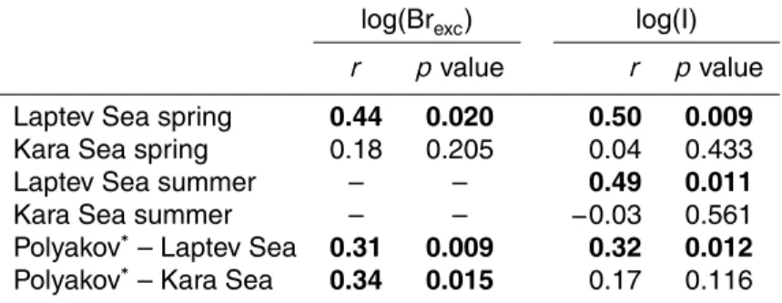
To understand the sources of air masses that influence the bromine and iodine de-position at the drill site of the Akademii Nauk ice core we calculated back trajecto-ries for the period covered by satellite sea ice measurements (1979–2000). Three-day back trajectories for spring (March, April, May, MAM) and six-Three-day back

trajecto-5

ries for summer (June, July, August; JJA) were calculated with the model HYSPLIT (HYbrid Single-Particle Lagrangian Integrated Trajectory, Version September 2014) us-ing NCEP/NCAR Reanalysis data from the National Weather Service’s National Cen-ters for Environmental Prediction provided by the NOAA’s Air Resources Laboratory (Draxler and Hess, 1998). The arrival height was the drilling site at Akademii Nauk ice

10

cap located at 760 m a.s.l. Trajectories were calculated each 12 h. Five-year averages were calculated for each three-month period (MAM and JJA) for the years 1980 to 2000 (Fig. 2).

2.4 Sea ice area and anomalies

Time series of the monthly mean sea ice area over the period January 1979 to

De-15

cember 2013 were calculated for three source regions in the Arctic (Fig. 1). These cor-respond to the Kara Sea (496 875 km2), the Laptev Sea (781 875 km2), and a subset of the Arctic Ocean (536 875 km2). Observations of sea ice concentrations from pas-sive microwave satellite radiometers were used as input data (Sea Ice Concentrations from Nimbus-7 SMMR and DMSP SSM/I-SSMIS Passive Microwave Data) (Cavalieri

20

et al., 1996, updated yearly). Regional averages were produced for the sea ice con-centration datasets which are published at 25 km grid resolution resulting in a single sea ice concentration value for each region every day. The time series were resampled to three-monthly averages for each region and averaged by multiplying the mean sea ice concentration with the area of each region.

25

(10)

con-TCD

9, 4407–4436, 2015

ice area

A. Spolaor et al.

Title Page

Tables Figures

◭ ◮

Back Close

Full Screen / Esc

Discussion

P

a

per

|

Discussion

P

a

per

|

Discussion

P

a

per

|

Discussion

P

a

per

|

centration range (greater uncertainty for lower ice concentrations). Although averaging over larger areas, such as those designated in Fig. 1, will reduce the relative uncer-tainty we estimate the unceruncer-tainty of the sea ice data presented here to be no greater than 10 %.

In addition to the satellite measurements we compare our results to the dataset

pro-5

duced by Polyakov et al. (2003) reporting August sea ice anomalies in the Kara, Laptev, East Siberian and Chukchi Seas. The dataset was produced by compiling Russian his-torical records of fast ice locations in the Arctic seas from ship-based observations, hy-drographic surveys and commercial shipping routes and aircraft-based observations. During World War II some missing data (1942–1945) were reconstructed using

statis-10

tical regression models.

3 Results

3.1 Trajectories and sea ice area: the Laptev Sea basin influence

Air mass back trajectories suggest that the Laptev Sea basin is the predominant source for air masses arriving at Akademii Nauk drill site during springtime (Fig. 2). The

per-15

centage of the springtime air masses originating in the Laptev basin range from a minimum of 44 % (1976–1980) up to 53 % (1991–1995), with the percentage of air masses originating from the Kara Sea and Arctic Ocean regions defined here consis-tently lower. Hence, we consider the Laptev Sea basin to be the most important source region for the spring climate signal present in the Akademii Nauk ice core. For the

20

summer period the sources are more variable with the Laptev Sea basin showing a majority of air mass sources in three of the five 5-year periods investigated. During the decade 1981–1990, the percentage of summer air masses from the Kara Sea exceeds those from the Laptev Sea (in particular between 1986–1990); however no associated changes have been detected in climate proxies such asδ18O (Opel et al., 2009).

(11)

TCD

9, 4407–4436, 2015

ice area

A. Spolaor et al.

Title Page

Tables Figures

◭ ◮

Back Close

Full Screen / Esc

Discussion

P

a

per

|

Discussion

P

a

per

|

Discussion

P

a

per

|

Discussion

P

a

per

|

In addition to the back trajectories we calculate sea ice areas for the three assigned basins of the Arctic Ocean and Laptev and Kara Sea regions. The results clearly demonstrate that the greatest variability of sea ice area occurs in the Laptev Sea for both spring and summer sea ice. In particular the Arctic Ocean region shows very small changes in summer minima and the production of first-year sea ice is hence negligible

5

compared to the other two basins. Seasonal changes in Kara Sea ice area are com-parable but smaller than those calculated for the Laptev Sea (Fig. 3). Considering that the air masses arriving at Akademii Nauk in spring and summer originate primarily from the Laptev Sea and that this region displays the greatest seasonal variability in sea ice area, we consider halogen concentrations in the Akademii Nauk ice core to be most

10

likely dominated by sea ice variability in the Laptev Sea. Nonetheless we also evaluate the possibility that the Kara Sea is an important secondary source of halogens.

3.2 Statistical analysis

Given the results of the calculated airmass back trajectory and observed sea ice vari-ability, we compare the yearly average values of Brexcand I concentrations with summer

15

and spring sea ice of Laptev and Kara Seas. Because of the low variability detected in this part of the Arctic Ocean, this region was excluded from statistical evaluation. Apart from the Polyakov anomalies, the parameters are transformed to the logarithmic scale to reduce their asymmetry and thus improve on the adherence to the normal distribu-tion assumpdistribu-tion used in the statistical analyses. Inspecdistribu-tion of normal probability plots

20

confirms the absence of departures from the normality for the log-transformed param-eters. Furthermore, the series of log(I) is de-trended by subtracting a least-squared-fit straight line. Autocorrelation and partial autocorrelation plots confirm the absence of serial correlation in the log-transformed parameters and in the detrended log(I).

Table 1 lists the correlations of the detrended log(I) and log(Brexc) with various

cal-25

culated parameters of sea ice extent together with thepvalues based on the unilateral

(12)

TCD

9, 4407–4436, 2015

ice area

A. Spolaor et al.

Title Page

Tables Figures

◭ ◮

Back Close

Full Screen / Esc

Discussion

P

a

per

|

Discussion

P

a

per

|

Discussion

P

a

per

|

Discussion

P

a

per

|

support a significant positive correlation between log(I) and the logarithm of the Laptev Sea ice area both in Spring (r₌0.50, df=20,p₌0.009) and Summer (r₌0.49, df=20,

p₌0.011), while there is no evidence of correlation with the Kara Sea ice area in either season. The results confirm also a positive correlation between log(Br_exc) and the log-arithm of the Laptev Sea spring sea ice (r₌0.44, df=20,p₌0.020) but not with Kara

5

Sea spring sea ice (r₌0.18, df=20,p₌0.205).

We also evaluate the correlation between Br_exc and I with the Polyakov anomalies dataset. The Polyakov anomalies dataset represents the summer (August) sea ice changes in the last century for several Arctic basins including the Laptev and Kara Seas. The obtained results confirm the finding that Br_excis correlated with Laptev and

10

Kara Sea ice. The correlation between log(Br_exc) and the Polyakov anomalies dataset is significant for both Laptev Sea sea ice (r₌0.34, df=48,pvalue=0.009) and Kara Sea sea ice (r₌0.31, df=48,p value=0.015). As regards iodine, data indicate a sig-nificant correlation between log(I) and the Polyakov anomalies data for Laptev Sea sea ice (r₌0.32, df=48,p value=0.012) but not for Kara Sea sea ice (r₌0.17, df=48,

15

pvalue=0.116). These results, together with back trajectory calculation, support the Laptev Sea as the main location of sea ice variability influencing Br_exc and I in the Akademii Nauk ice core.

4 Discussion

4.1 Brexcand Laptev Sea spring sea ice

20

Bromine explosions are defined as the autocatalytic sequence of chemical reactions able to generate gas phase bromine (such as BrO) and they occur mainly above seasonal sea ice (Fig. 4). Br explosions lead to enrichment of Br in snow depo-sition, well beyond the Br/Na ratio observed in seawater. There are two calcula-tions that can be used to quantify the influence of bromine explosions in snowpack:

25

(13)

TCD

9, 4407–4436, 2015

ice area

A. Spolaor et al.

Title Page

Tables Figures

◭ ◮

Back Close

Full Screen / Esc

Discussion

P

a

per

|

Discussion

P

a

per

|

Discussion

P

a

per

|

Discussion

P

a

per

|

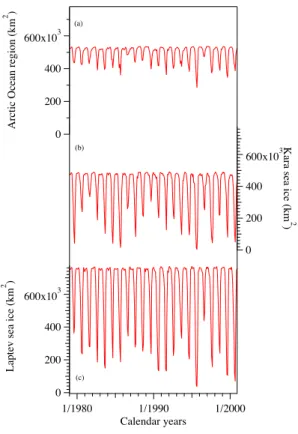
Br / Na seawater concentration ratio of 0.006 (Turekian, 1968). Br_exc is calculated as Brexc=[Br]−[Na]×0.006 and indicates how much bromine has been produced by the

bromine explosion. Brenr is calculated as Brenr=[Br] / ([Na]×0.006) and indicates the

proportion to which bromine has been enriched beyond the seawater ratio. Compar-ing both Br indicators (Brexc and Brenr) reveals that they have a similar trend over the

5

past 50 years, with a peak in the 1970s and 1980s and a sharp decrease in the last decade of the record (Fig. 5). To investigate the connection between Br and sea ice we used Brexc since it allows quantification of the additional bromine fluxes produced by

the bromine explosion. Additionally, the Akademii Nauk ice core was subject to sum-mer melt and hence may be susceptible to artefacts based on the different percolation

10

velocities of Br and Na. Air mass back trajectory data indicate the Laptev Sea is the pri-mary springtime source of air masses arriving at Akademii Nauk so we compare Brexc

with spring sea ice area in the Laptev Sea. A strong influence of the bromine explosion also is expected due to the observation that only 15 to 30 % of sea ice is present by late summer, implying that almost all spring sea ice is seasonal. Furthermore, Laptev Sea

15

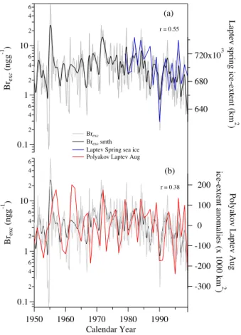
ice can be exported by the Transpolar Drift through the Arctic Ocean to the Greenland Sea and North Atlantic, leading to strong recycling of sea ice in the area (Xiao et al., 2013). Comparing Brexc and Laptev Sea spring sea ice we find a positive correlation

(r₌0.44). Over the period for which observations are available, noting that both spring sea ice area and Br_exc exhibit a steadily decreasing trend (Fig. 6a). In 1991 in

particu-20

lar, we observe a sharp decrease of spring sea ice followed by decreasing production of Brexc. The intensity of bromine explosion and the production of BrO in the Arctic

are strongly driven by sea ice presence, in this case spring sea ice. Br_exc also was compared with a 50-year record of summer (August) sea ice anomalies for the Laptev basin, calculated by Polyakov et al. (2003) (Fig. 6b). We found a positive correlation

25

between the two data series (r₌0.31). We emphasize that the degree of correlation may be influenced by the fact that we are not comparing Brexcto the sea ice area at the

(14)

TCD

9, 4407–4436, 2015

ice area

A. Spolaor et al.

Title Page

Tables Figures

◭ ◮

Back Close

Full Screen / Esc

Discussion

P

a

per

|

Discussion

P

a

per

|

Discussion

P

a

per

|

Discussion

P

a

per

|

here. Although our results suggest that excess of Br in snow deposition seem mainly driven by the changes in sea ice area, especially first year sea ice, we also consider other factors that could contribute to the total nss-Br in the snow deposition. Bromine explosions are catalyzed by acidity and light, and a change in the acidic condition of the Arctic atmosphere could produce a change in the magnitude of bromine activation

5

and hence bromine deposition (Sander et al., 2006). Quantification of the impacts of acidity changes on Br_exc (or Br_enr) deposition is beyond the scope of this study and additional studies are necessary to better understand which factors (e.g. sea ice area, acidity, wind pumping, temperature) are the most relevant. However the highly signif-icant correlations and previous research suggests that sea ice is the main driver of

10

Br_exc.

4.2 Iodine and Laptev Sea summer sea ice

While the main source of iodine in Antarctica has been attributed to sea ice algae dur-ing sprdur-ing time (Atkinson et al., 2012) and recently also to inorganic emissions durdur-ing winter time (Granfors et al., 2015), in the Arctic there is a lack of knowledge regarding

15

iodine sources. One of the main barriers to identifying Arctic iodine sources is that the atmospheric concentrations of IO are close to satellite detection limits (Fig. 4). The first measurements of iodine in aerosols were presented by Sturges and Barrie (1988) and they found increasing concentrations during late spring and summer. More recently Mahajan et al. (2010) detected iodine emissions in the form of IO, related to the

pres-20

ence of polynyas or areas free of sea ice. These open water areas were identified as hot spots for iodine emission. Arctic sea ice is thicker and less permeable than Antarc-tic sea ice, constituting a barrier between the ocean and the atmosphere (Zhou et al., 2013). In this case it is likely that gas phase iodine produced from sea ice algae could escape only from sea ice leads (cracks) or the open ocean surface. The Akademii Nauk

25

(15)

TCD

9, 4407–4436, 2015

ice area

A. Spolaor et al.

Title Page

Tables Figures

◭ ◮

Back Close

Full Screen / Esc

Discussion

P

a

per

|

Discussion

P

a

per

|

Discussion

P

a

per

|

Discussion

P

a

per

|

Laptev basin calculated by Polyakov et al. (2003) (Fig. 7b). A significant positive corre-lation (r₌0.32, Table 1) was observed also in this case. No significant correlation was observed with summer or spring sea ice area in the Kara Sea (Table 1), supporting the back-trajectory analysis data. These results are consistent with iodine concentrations from a snow pit sampled at the NEEM ice core site in northwest Greenland. The NEEM

5

record displayed peak iodine concentrations in summer (Spolaor et al., 2014), although only three annual cycles were sampled. In contrast, iodine concentrations from Sval-bard were more consistent with spring sea ice area (Spolaor et al., 2013a). The results from Svalbard must be evaluated with caution because seasonal variability is less clear in the Svalbard records and the influence of summer melting and iodine re-emission

10

may be more significant than for the Akademii Nauk ice core. The summer peak of io-dine concentrations found in Arctic snow and ice depends upon both the production of iodine by sea ice algae and processes that control release of iodine to the atmosphere. Arctic sea ice is an e_ffective barrier to gas exchange in the ocean-atmosphere system especially in winter, when there is low ice permeability and minimal convection of Arctic

15

waters (Zhou et al., 2013). Ice permeability follows Arctic temperatures, with maximum permeability in summer and particularly when the sea ice is warmer than−5◦C.

Wa-ter convection is greatest during spring, driven by an unstable brine density profile. Fracturing is an additional process that may enhance gas exchange, and hence iodine emission from the Arctic Seas, particularly in the highly dynamic Laptev Sea.

Phyto-20

plankton blooms occur mainly in late spring and summer (Ardyna et al., 2013; Arrigo et al., 2012), responding to the availability of nutrients and the limited penetration of light through thick winter sea ice. These factors ensure that the most e_fficient season for production and emission of iodine is the Arctic summer. In summer, the decreased sea ice thickness, increased sea ice fracturing and permeability, and enhanced light

pene-25

(16)

TCD

9, 4407–4436, 2015

ice area

A. Spolaor et al.

Title Page

Tables Figures

◭ ◮

Back Close

Full Screen / Esc

Discussion

P

a

per

|

Discussion

P

a

per

|

Discussion

P

a

per

|

Discussion

P

a

per

|

available from Greenland (Spolaor et al., 2014) and presented here for the Akademii Nauk ice core. Satellite measurements of Arctic IO concentrations exceed detection limits only in the summer, and at that time of maximum IO concentrations above sum-mer sea ice. Improved sensitivity of satellite-borne instruments would greatly enhance the detection and seasonal variability of IO emission sources in the Arctic.

5

5 Conclusions

The halogens iodine and bromine reported here from the Akademii Nauk ice core from Severnaya Zemlya offer a new perspective on the variability of sea ice in the Arctic. Previous work suggests a connection of bromine and iodine chemistry with sea ice changes (Spolaor et al., 2013a, b, 2014). In particular, Br_excand Br_enrhave been linked

10

to seasonal sea ice area and here we report a connection between ice-core Brexc and

spring sea ice in the Laptev Sea largely because almost all Laptev Sea spring sea ice is seasonal (approximately 80 %) and so undergoes continuous renewal. Ice-core iodine appears to be connected with the summer sea ice area; however, its sources are biologically-mediated making the interpretation more difficult and atmospheric

con-15

centrations of IO in the Arctic are close to satellite detection limits, limiting the accurate characterization of IO emission sources. Further studies are necessary to better iden-tify the seasonal variability of this element and the impact of acidity on bromine reactiv-ity in Arctic. However, the significant correlation between nss-Br and sea ice during the last 50 years in the Akademii Nauk ice-core record suggests that the nss-Br record

pri-20

(17)

TCD

9, 4407–4436, 2015

ice area

A. Spolaor et al.

Title Page

Tables Figures

◭ ◮

Back Close

Full Screen / Esc

Discussion

P

a

per

|

Discussion

P

a

per

|

Discussion

P

a

per

|

Discussion

P

a

per

|

The Supplement related to this article is available online at doi:10.5194/tcd-9-4407-2015-supplement.

Acknowledgements. This study contributes to the Eurasian Arctic Ice 4k project and was

sup-ported by the Deutsche Forschungsgemeinschaft (grant OP 217/2-1 awarded to Thomas Opel). The drilling project on Akademii Nauk ice cap has been funded by German Ministry of

Educa-5

tion and Research (BMBF research project 03PL 027A). Analysis and interpretation of the Akademii Nauk ice core at the Desert Research Institute was funded by US National Science Foundation grant 1023672. Paul Vallelonga has received funding from the European Research Council under the European Union’s Seventh Framework Programme (FP7/2007-2013)/ERC grant agreement no. 610055 “Ice2Ice”. We thank the University of Bremen, supported by the

10

State of Bremen, the German Aerospace, DLR and the European Space Agency for the satellite BrO imagines.

References

Abram, N. J., Wolff, E. W., and Curran, M. A. J.: A review of sea ice proxy information from polar ice cores, Quaternary Sci. Rev., 79, 168–183, doi:10.1016/j.quascirev.2013.01.011, 2013.

15

Allan, J. D., Williams, P. I., Najera, J., Whitehead, J. D., Flynn, M. J., Taylor, J. W., Liu, D., Darbyshire, E., Carpenter, L. J., Chance, R., Andrews, S. J., Hackenberg, S. C., and McFig-gans, G.: Iodine observed in new particle formation events in the Arctic atmosphere during ACCACIA, Atmos. Chem. Phys., 15, 5599–5609, doi:10.5194/acp-15-5599-2015, 2015. Ardyna, M., Babin, M., Gosselin, M., Devred, E., Bélanger, S., Matsuoka, A., and Tremblay,

20

J.-É.: Parameterization of vertical chlorophyll a in the Arctic Ocean: impact of the subsur-face chlorophyll maximum on regional, seasonal, and annual primary production estimates, Biogeosciences, 10, 4383–4404, doi:10.5194/bg-10-4383-2013, 2013.

Arrigo, K. R., Perovich, D. K., Pickart, R. S., Brown, Z. W., van Dijken, G. L., Lowry, K. E., Mills, M. M., Palmer, M. A., Balch, W. M., Bahr, F., Bates, N. R., Benitez-Nelson, C., Bowler, B.,

25

(18)

Phyto-TCD

9, 4407–4436, 2015

ice area

A. Spolaor et al.

Title Page

Tables Figures

◭ ◮

Back Close

Full Screen / Esc

Discussion

P

a

per

|

Discussion

P

a

per

|

Discussion

P

a

per

|

Discussion

P

a

per

|

plankton Blooms Under Arctic Sea Ice, Science, 336, 1408, doi:10.1126/science.1215065, 2012.

Atkinson, H. M., Huang, R.-J., Chance, R., Roscoe, H. K., Hughes, C., Davison, B., Schönhardt, A., Mahajan, A. S., Saiz-Lopez, A., Hoffmann, T., and Liss, P. S.: Iodine emissions from the sea ice of the Weddell Sea, Atmos. Chem. Phys., 12, 11229–11244,

doi:10.5194/acp-12-5

11229-2012, 2012.

Belt, S. T., Massé, G., Rowland, S. J., Poulin, M., Michel, C., and LeBlanc, B.: A novel chemical fossil of palaeo sea ice: IP25, Organ. Geochem., 38, 16–27, 2007.

Comiso, J. C.: Large Decadal Decline of the Arctic Multiyear Ice Cover, J. Climate, 25, 1176– 1193, doi:10.1175/jcli-d-11-00113.1, 2011.

10

Curran, M. A., Van Ommen, T. D., Morgan, V. I., Phillips, K. L., and Palmer, M. R.: Ice core evidence for Antarctic sea ice decline since the 1950s, Science, 302, 1203–1206, 2003. Darby, D. A.: Sources of sediment found in sea ice from the western Arctic Ocean, new

in-sights into processes of en- trainment and drift patterns, J. Geophys. Res., 108, 3257, doi:10.1029/2002JC001350, 2003.

15

Dieckmann, G. S. and Hellmer, H. H.: The Importance of Sea Ice: An Overview, in Sea Ice, Wiley-Blackwell, 1–22, 2009.

Divine, D. V. and Dick, C.: Historical variability of sea ice edge position in the Nordic Seas, J. Geophys. Res.-Oceans, 111, C01001, doi:10.1029/2004jc002851, 2006.

Draxler, R. R. and Hess, G. D.: An overview of the HYSPLIT_4 modeling system of trajectories,

20

dispersion, and deposition, Aust. Meteorol. Mag., 47, 295–308, 1998.

Francis, J. A., Chan, W., Leathers, D. J., Miller, J. R., and Veron, D. E.: Winter Northern Hemi-sphere weather patterns remember summer Arctic sea-ice extent, Geophys. Res. Lett., 36, L07503, doi:10.1029/2009GL037274, 2009.

Fritzsche, D., Wilhelms, F., Savatyugin, L. M., Pinglot, J. F., Meyer, H., Hubberten, H. W., and

25

Miller, H.: A new deep ice core from Akademii Nauk ice cap, Severnaya Zemlya, Eurasian Arctic: first results, Ann. Glaciol., 35, 25–28, 2002.

Fritzsche, D., Schütt, R., Meyer, H., Miller, H., Wilhelms, F., Opel, T., and Savatyugin, L. M.: A 275 year ice-core record from Akademii Nauk ice cap, Severnaya Zemlya, Russian Arctic, Ann. Glaciol., 42, 361–366, 2005.

30

(19)

TCD

9, 4407–4436, 2015

ice area

A. Spolaor et al.

Title Page

Tables Figures

◭ ◮

Back Close

Full Screen / Esc

Discussion

P

a

per

|

Discussion

P

a

per

|

Discussion

P

a

per

|

Discussion

P

a

per

|

Holland, M. M., Bitz, C. M., Eby, M., and Weaver, A. J.: The Role of Ice-Ocean Interactions in the Variability of the North Atlantic Thermohaline Circulation, J. Climate, 14, 656–675, 2001. Isaksson, E., Kekonen, T., Moore, J., and Mulvaney, R.: The methanesulfonic acid (MSA) record

in a Svalbard ice core, Ann. Glaciol., 42, 345–351, 2005.

Kinnard, C., Zdanowicz, C. M., Fisher, D. A., Isaksson, E., De Vernal, A., and Thompson, L. G.:

5

Reconstructed changes in Arctic sea ice over the past 1,450 years, Nature, 479, 509–512, 2011.

Levine, J. G., Yang, X., Jones, A. E., and Wol, E. W.: Sea salt as an ice core proxy for past sea ice extent: A process-based model study, J. Geophys. Res.-Atmos., 119, 2013JD020925, doi:10.1002/2013jd020925, 2014.

10

Lisitzin, A. P.: Sea-ice and Iceberg Sedimentation in the Ocean: Recent and Past, Springer-Verlag, Berlin, Heidelberg, 2002.

Mahajan, A. S., Shaw, M., Oetjen, H., Hornsby, K. E., Carpenter, L. J., Kaleschke, L., Tian-Kunze, X., Lee, J. D., Moller, S. J., Edwards, P., Commane, R., Ingham, T., Heard, D. E., and Plane, J. M. C.: Evidence of reactive iodine chemistry in the Arctic boundary layer, J.

15

Geophys. Res.-Atmos., 115, D20303, doi:10.1029/2009jd013665, 2010.

Maselli, O. J., Fritzsche, D., Layman, L., McConnell, J. R., and Meyer, H.: Comparison of wa-ter isotoperatio dewa-terminations using two cavity ring-down instruments and classical mass spectrometry in continuous ice-core analysis, Isotopes Environ. Health Stud., 49, 387–398, doi:10.1080/10256016.2013.781598, 2013.

20

McConnell, J. R., Lamorey, G. W., Lambert, S. W., and Taylor, K. C.: Continuous Ice-Core Chemical Analyses Using Inductively Coupled Plasma Mass Spectrometry, Environ. Sci. Technol., 36, 7–11, doi:10.1021/es011088z, 2002.

McConnell, J. R., Edwards, R., Kok, G. L., Flanner, M. G., Zender, C. S., Saltzman, E. S., Banta, J. R., Pasteris, D. R., Carter, M. M., and Kahl, J. D. W.: 20th-Century Industrial Black Carbon

25

Emissions Altered Arctic Climate Forcing, Science, 317, 1381–1384, 2007.

McConnell, J. R., Maselli, O. J., Sigl, M., Vallelonga, P., Neumann, T., Anschütz, H., Bales, R. C., Curran, M. A. J., Das, S. B., Edwards, R., Kipfstuhl, S., Layman, L., and Thomas, E. R.: Antarcticwide array of high-resolution ice core records reveals pervasive lead pollution began in 1889 and persists today. Scientific Reports, 4, 5848, doi:10.1038/srep05848, 2014.

30

(20)

TCD

9, 4407–4436, 2015

ice area

A. Spolaor et al.

Title Page

Tables Figures

◭ ◮

Back Close

Full Screen / Esc

Discussion

P

a

per

|

Discussion

P

a

per

|

Discussion

P

a

per

|

Discussion

P

a

per

|

Opel, T., Fritzsche, D., Meyer, H., Schütt, R., Weiler, K., Ruth, U., Wilhelms, F., and Fischer, H.: 115 year ice-core data from Akademii Nauk ice cap, Severnaya Zemlya: high-resolution record of Eurasian Arctic climate change, J. Glaciol., 55, 21–31, 2009.

Opel, T., Fritzsche, D., and Meyer, H.: Eurasian Arctic climate over the past millennium as recorded in the Akademii Nauk ice core (Severnaya Zemlya), Clim. Past, 9, 2379–2389,

5

doi:10.5194/cp-9-2379-2013, 2013.

Pasteris, D. R., McConnell, J. R., Das, S. B., Criscitiello, A. S., Evans, M. J., Maselli, O. J., Sigl, M., and Layman, L.: Seasonally resolved ice core records from West Antarctica indicate a sea ice source of sea-salt aerosol and a biomass burning source of ammonium, J. Geophys. Res.-Atmos., doi:10.1002/2013jd020720, in press, 2014.

10

Petit, J. R., Jouzel, J., Raynaud, D., Barkov, N. I., Barnola, J. M., Basile, I., Bender, M., Chap-pellaz, J., Davis, M., Delaygue, G., Delmotte, M., Kotlyakov, V. M., Legrand, M., Lipenkov, V. Y., Lorius, C., Pepin, L., Ritz, C., Saltzman, E., and Stievenard, M.: Climate and atmospheric history of the past 420,000 years from the Vostok ice core, Antarctica, Nature, 399, 429–436, 1999.

15

Pohjola, V. A., Moore, J. C., Isaksson, E., Jauhiainen, T., Van de Wal, R. S. W., Martma, T., Meijer, H. A. J., and Vaikmäe, R.: Effect of periodic melting on geochemical and isotopic signals in an ice core from Lomonosovfonna, Svalbard, J. Geophys. Res.-Atmos., 107, 1–14, 2002.

Polyak, L., Alley, R. B., Andrews, J. T., Brigham-Grette, J., Cronin, T. M., Darby, D. A., Dyke,

20

A. S., Fitzpatrick, J. J., Funder, S., Holland, M., Jennings, A. E., Miller, G. H., O’Regan, M., Savelle, J., Serreze, M., St. John, K., White, J. W. C., and Wolff, E.: History of sea ice in the Arctic, Quaternary Sci. Rev., 29, 1757–1778, 2010.

Polyakov, I. V., Alekseev, G. V., Bekryaev, R. V., Bhatt, U. S., Colony, R., Johnson, M. A., Karklin, V. P., Walsh, D., and Yulin, A. V.: Long-term ice variability in Arctic marginal seas, J. Climate,

25

16, 2078–2085, 2003.

Pratt, K. A., Custard, K. D., Shepson, P. B., Douglas, T. A., Pohler, D., General, S., Zielcke, J., Simpson, W. R., Platt, U., Tanner, D. J., Gregory Huey, L., Carlsen, M., and Stirm, B. H.: Photochemical production of molecular bromine in Arctic surface snowpacks, Nat. Geosci., 6, 351–356, doi:10.1038/ngeo1779, 2013.

30

(21)

TCD

9, 4407–4436, 2015

ice area

A. Spolaor et al.

Title Page

Tables Figures

◭ ◮

Back Close

Full Screen / Esc

Discussion

P

a

per

|

Discussion

P

a

per

|

Discussion

P

a

per

|

Discussion

P

a

per

|

Saiz-Lopez, A., Mahajan, A. S., Salmon, R. A., Bauguitte, S. J. B., Jones, A. E., Roscoe, H. K., and Plane, J. M. C.: Boundary Layer Halogens in Coastal Antarctica, Science, 317, 348–351, 2007.

Sander, R., Burrows, J., and Kaleschke, L.: Carbonate precipitation in brine – a poten-tial trigger for tropospheric ozone depletion events, Atmos. Chem. Phys., 6, 4653–4658,

5

doi:10.5194/acp-6-4653-2006, 2006.

Schönhardt, A., Begoin, M., Richter, A., Wittrock, F., Kaleschke, L., Gómez Martín, J. C., and Burrows, J. P.: Simultaneous satellite observations of IO and BrO over Antarctica, Atmos. Chem. Phys., 12, 6565–6580, doi:10.5194/acp-12-6565-2012, 2012.

Sigl, M., McConnell, J. R., Toohey, M., Curran, M., Das, S. B., Edwards, R., Isaksson, E.,

10

Kawamura, K., Kipfstuhl, S., Kruger, K., Layman, L., Maselli, O. J., Motizuki, Y., Motoyama, H., Pasteris, D. R., and Severi, M.: Insights from Antarctica on volcanic forcing during the Common Era, Nat. Clim. Change, 4, 693–697, doi:10.1038/nclimate2293, 2014.

Simpson, W. R., Carlson, D., Hönninger, G., Douglas, T. A., Sturm, M., Perovich, D., and Platt, U.: First-year sea-ice contact predicts bromine monoxide (BrO) levels at Barrow, Alaska

bet-15

ter than potential frost flower contact, Atmos. Chem. Phys., 7, 621–627, doi:10.5194/acp-7-621-2007, 2007.

Spolaor, A., Gabrieli, J., Martma, T., Kohler, J., Björkman, M. B., Isaksson, E., Varin, C., Valle-longa, P., Plane, J. M. C., and Barbante, C.: Sea ice dynamics influence halogen deposition to Svalbard, The Cryosphere, 7, 1645–1658, doi:10.5194/tc-7-1645-2013, 2013a.

20

Spolaor, A., Vallelonga, P., Plane, J. M. C., Kehrwald, N., Gabrieli, J., Varin, C., Turetta, C., Cozzi, G., Kumar, R., Boutron, C., and Barbante, C.: Halogen species record Antarc-tic sea ice extent over glacial-interglacial periods, Atmos. Chem. Phys., 13, 6623–6635, doi:10.5194/acp-13-6623-2013, 2013b.

Spolaor, A., Vallelonga, P., Gabrieli, J., Martma, T., Björkman, M. P., Isaksson, E., Cozzi, G.,

25

Turetta, C., Kjær, H. A., Curran, M. A. J., Moy, A. D., Schönhardt, A., Blechschmidt, A. M., Burrows, J. P., Plane, J. M. C., and Barbante, C.: Seasonality of halogen deposition in polar snow and ice, Atmos. Chem. Phys., 14, 9613–9622, doi:10.5194/acp-14-9613-2014, 2014. Stroeve, J., Holland, M. M., Meier, W., Scambos, T., and Serreze, M.: Arctic sea ice decline:

Faster than forecast, Geophys. Res. Lett., 34, L09501, doi:10.1029/2007GL029703, 2007.

30

(22)

TCD

9, 4407–4436, 2015

ice area

A. Spolaor et al.

Title Page

Tables Figures

◭ ◮

Back Close

Full Screen / Esc

Discussion

P

a

per

|

Discussion

P

a

per

|

Discussion

P

a

per

|

Discussion

P

a

per

|

Sturges, W. T. and Harrison, R. M.: Bromine in marine aerosols and the origin, nature and quantity of natural atmospheric bromine, Atmos. Environ., 20, 1485–1496, 1986.

Turekian, K. K.: Oceans, edited by: Englewood, C., Prentice-Hall, N. J., 1968.

Turner, J., Bracegirdle, T., Phillips, T., Marshall, G. J., and Hosking, J. S.: An Initial Assessment of Antarctic Sea Ice Extent in the CMIP5 Models, J. Climate, 26, 1473–1484, 2012.

5

Vinje, T.: Anomalies and Trends of Sea-Ice Extent and Atmospheric Circulation in the Nordic Seas during the Period 1864–1998, J. Climate, 14, 255–267, doi:10.1175/1520-0442(2001)014<0255:aatosi>2.0.co;2, 2001.

Vogt, R., Crutzen, P. J., and Sander, R.: A mechanism for halogen release from sea-salt aerosol in the remote marine boundary layer, Nature, 383, 327–330, 1996.

10

Weiler, K., Fischer, H., Fritzsche, D., Ruth, U., Wilhelms, F., and Miller, H.: Glaciochemical reconnaissance of a new ice core from Severnaya Zemlya, Eurasian Arctic, Ann. Glaciol., 51, 64–74, 2005.

Wol_ff, E. W., Fischer, H., Fundel, F., Ruth, U., Twarloh, B., Littot, G. C., Mulvaney, R., Roth-lisberger, R., de Angelis, M., Boutron, C. F., Hansson, M., Jonsell, U., Hutterli, M. A.,

Lam-15

bert, F., Kaufmann, P., Stauffer, B., Stocker, T. F., Steffensen, J. P., Bigler, M., Siggaard-Andersen, M. L., Udisti, R., Becagli, S., Castellano, E., Severi, M., Wagenbach, D., Barbante, C., Gabrielli, P., and Gaspari, V.: Southern Ocean sea-ice extent, productivity and iron flux over the past eight glacial cycles, Nature, 440, 491–496, 2006.

Wolff, E. W., Barbante, C., Becagli, S., Bigler, M., Boutron, C. F., Castellano, E., De Angelis, M.,

20

Federer, U., Fischer, H., and Fundel, F.: Changes in environment over the last 800,000 years from chemical analysis of the EPICA Dome C ice core, Quaternary Sci. Rev., 29, 285–295, 2010.

Xiao, X., Fahl, K., and Stein, R.: Biomarker distributions in surface sediments from the Kara and Laptev seas (Arctic Ocean): indicators for organic-carbon sources and sea-ice coverage,

25

Quarternary Sci. Rev., 79 40–52, 2013.

Zhou, J., Delille, B., Eicken, H., Vancoppenolle, M., Brabant, F., Carnat, G., Geilfus, N.-X., Papakyriakou, T., Heinesch, B., and Tison, J.-L.: Physical and biogeochemical properties in land- fast sea ice (Barrow, Alaska): Insights on brine and gas dynamics across seasons, J. Geophys. Res.-Oceans, 118, 3172–3189, doi:10.1002/jgrc.20232, 2013.

(23)

TCD

9, 4407–4436, 2015

ice area

A. Spolaor et al.

Title Page

Tables Figures

◭ ◮

Back Close

Full Screen / Esc

Discussion

P

a

per

|

Discussion

P

a

per

|

Discussion

P

a

per

|

Discussion

P

a

per

|

Table 1.Correlations (r) of the detrended log(I) and log(Br_exc) with the logarithm of the first year sea ice area in the Laptev and Kara seas for the period 1979–1999 and the Polyakov anomalies in the Laptev and Kara seas for the period 1950–1999 (denoted by an asterisk∗) (Polyakov et al., 2003). Columns display ther values andpvalues. Bold numbers indicate the statistically significant correlations.

log(Br_exc) log(I)

r pvalue r pvalue

Laptev Sea spring 0.44 0.020 0.50 0.009

Kara Sea spring 0.18 0.205 0.04 0.433

Laptev Sea summer – – 0.49 0.011

Kara Sea summer – – ₋0.03 0.561

(24)

TCD

9, 4407–4436, 2015

ice area

A. Spolaor et al.

Title Page

Tables Figures

◭ ◮

Back Close

Full Screen / Esc

Discussion

P

a

per

|

Discussion

P

a

per

|

Discussion

P

a

per

|

Discussion

P

a

per

|

(25)

TCD

9, 4407–4436, 2015

ice area

A. Spolaor et al.

Title Page

Tables Figures

◭ ◮

Back Close

Full Screen / Esc

Discussion

P

a

per

|

Discussion

P

a

per

|

Discussion

P

a

per

|

Discussion

P

a

per

|

1976 - 1980

1996 - 2000

1 ( 58%) 2 ( 30%)

l

3 ( 13% )

1991 - 1995 1986 - 1990 1981 - 1985

1 ( 27% ) 2 ( 38%)

3 ( 35%)

1 ( 54%) 2 ( 17%)

3 ( 29%)

1 ( 29%) 2 ( 20%)

3 ( 51%) March - April - May (MAM) June - July - August (JJA)

s

1 ( 40%) _{2 ( 47% )}

l

3 ( 12%)

s s

1 ( 42%) 2 ( 14%)

3 ( 44%)

1 ( 45%) 2 ( 44%)

3 ( 11%)

1 ( 37%) 2 ( 14% )

3 ( 48% )

70

1 ( 30%)

2 ( 17% )

3 ( 53%)

1 ( 23%) 2 ( 26%)

3 ( 52%)

(26)

TCD

9, 4407–4436, 2015

ice area

A. Spolaor et al.

Title Page

Tables Figures

◭ ◮

Back Close

Full Screen / Esc

Discussion

P

a

per

|

Discussion

P

a

per

|

Discussion

P

a

per

|

Discussion

P

a

per

|

600x103

400

200

0

Laptev sea ice (km

2 )

1/1980 1/1990 1/2000

Calendar years

600x103

400

200

0

Kara sea ice (km

2

)

600x103

400

200

0

Arctic Ocean region (km

2 )

(a)

(b)

(c)

Figure 3.Sea ice area variation in the period 1979–2000 for the three regions defined in Fig. 1;

(27)

TCD

9, 4407–4436, 2015

ice area

A. Spolaor et al.

Title Page

Tables Figures

◭ ◮

Back Close

Full Screen / Esc

Discussion

P

a

per

|

Discussion

P

a

per

|

Discussion

P

a

per

|

Discussion

P

a

per

|

(28)

TCD

9, 4407–4436, 2015

ice area

A. Spolaor et al.

Title Page

Tables Figures

◭ ◮

Back Close

Full Screen / Esc

Discussion

P

a

per

|

Discussion

P

a

per

|

Discussion

P

a

per

|

Discussion

P

a

per

|

7

0.1

2 3 4 5 6 7

1

2 3 4 5 6 7

10

2 3 4 5 6 7

Br

exc

(ngg

-1 )

1990 1980

1970 1960

1950

Calendar Year

3 4 5 6 7 8

91

2 3 4 5 6 7 8

910

2 3 4 5

Br

enr

Brexc

Brenr

Brenr smth

(29)

TCD

9, 4407–4436, 2015

ice area

A. Spolaor et al.

Title Page

Tables Figures

◭ ◮

Back Close

Full Screen / Esc

Discussion

P

a

per

|

Discussion

P

a

per

|

Discussion

P

a

per

|

Discussion

P

a

per

|

0.1

2 4 6

1

2 4 6

10

2 4 6

Br

exc

(ngg

-1 )

1990 1980 1970 1960 1950

Calendar Year

720x103

680

640

Laptev spring ice-extent (km

2

)

0.1

2 4 6

1

2 4 6

10

2 4 6

Br

exc

(ngg

-1 )

-300 -200 -100

0 100 200

Polyakov Laptev Aug

ice-extent anomalies (x 1000 km

2

)

(a)

(b)

r = 0.55

r = 0.38

Brexc

Brexc smth

Laptev Spring sea ice Polyakov Laptev Aug

(30)

TCD

9, 4407–4436, 2015

ice area

A. Spolaor et al.

Title Page

Tables Figures

◭ ◮

Back Close

Full Screen / Esc

Discussion

P

a

per

|

Discussion

P

a

per

|

Discussion

P

a

per

|

Discussion

P

a

per

|

6 0.01

2 4 6 0.1

2 4 6 1

2

I (ngg

-1 )

1990 1980 1970 1960 1950

Calendar Year

550x103

500

450

400

350

300

Laptev summer ice-extent (km

2

)

2 4 6 0.1

2 4 6 1

2 4

I (ngg

-1 )

-300 -200 -100

0 100

200 _{Polyakov Laptev Aug}

ice-extent anomalies ( x 1000 Km

2

)

(a)

(b) r = 0.50

r = 0.32

I (ngg-1)

I (ngg-1) smth

Laptev Summer sea ice Polyakov Laptev Aug