www.biogeosciences.net/11/2925/2014/ doi:10.5194/bg-11-2925-2014
© Author(s) 2014. CC Attribution 3.0 License.
Pumping methane out of aquatic sediments – ebullition forcing
mechanisms in an impounded river
A. Maeck1, H. Hofmann2, and A. Lorke1
1University of Koblenz-Landau, Institute for Environmental Sciences, Fortstr. 7, 76829 Landau, Germany 2University of Konstanz, Limnological Institute, Mainaustr. 252, 78464 Konstanz, Germany
Correspondence to: A. Maeck (maeck@uni-landau.de)
Received: 4 September 2013 – Published in Biogeosciences Discuss.: 28 November 2013 Revised: 27 March 2014 – Accepted: 27 March 2014 – Published: 5 June 2014
Abstract. Freshwater systems contribute significantly to the global atmospheric methane budget. A large fraction of the methane emitted from freshwaters is transported via ebulli-tion. However, due to its strong variability in space and time, accurate measurements of ebullition rates are difficult; hence, the uncertainty regarding its contribution to global budgets is large. Here, we analyze measurements made by contin-uously recording automated bubble traps in an impounded river in central Europe and investigate the mechanisms af-fecting the temporal dynamics of bubble release from cohe-sive sediments. Our results show that the main triggers of bubble release were pressure changes, originating from the passage of ship lock-induced surges and ship passages. The response to physical forcing was also affected by previous outgassing. Ebullition rates varied strongly over all relevant timescales from minutes to days; therefore, representative ebullition estimates could only be inferred with continuous sampling over long periods. Since ebullition was found to be episodic, short-term measurement periods of a few hours or days will likely underestimate ebullition rates. Our results thus indicate that flux estimates could be grossly underesti-mated (by up to ~ 50%) if the correct temporal resolution is not used during data collection.
1 Introduction
Methane (CH4)is regarded as the second-most important an-thropogenic greenhouse gas, with global emission rates be-tween 500 and 600 Tg yr−1(Forster et al., 2007). The con-tribution of freshwater systems is estimated to be around
103 Tg CH4yr−1, of which over 53 % is emitted via gas bub-bles (Bastviken et al., 2011).
Gas bubbles released from anoxic freshwater sediments often consist of a large proportion of CH4 (Baulch et al., 2011). In these sediments where alternative electron accep-tors, e.g., nitrate or sulfate, are lacking or depleted and degradable organic carbon (Corg) is available, CH4 is duced by organisms of the domain archaea. The rate of pro-duction depends on the amount and quality of Corgand tem-perature (Duc et al., 2010; Liikanen and Martikainen, 2003; Segers, 1998; Sobek et al., 2012). Produced CH4can dissolve into the porewater, and thus continuous production in combi-nation with low efflux rates can lead to high concentrations of CH4within the porewater (Maeck et al., 2013). If the par-tial pressure of all dissolved gases in the porewater exceeds the ambient pressure and the surface tension of water, free gas is formed. Due to ongoing production of CH4, bubbles within the sediments grow and form fractures or disc-shaped cavities (Boudreau et al., 2005; Johnson et al., 2002).
where O2, NO−3 or SO24−is present, a larger fraction of the free CH4gas can re-dissolve and be oxidized (Venkiteswaran et al., 2013). In terms of atmospheric emissions, physical and chemical parameters like the water depth, bubble size and the concentration of CH4 in the ambient water determine what fraction of the initially released CH4reaches the atmosphere (Leifer and Patro, 2002; McGinnis et al., 2006). Although it varies with depth and environmental conditions, the fate of rising CH4 bubbles in the water column is well under-stood (Leifer and Patro, 2002; McGinnis et al., 2006), stud-ies investigating the mechanisms responsible for the tempo-ral and spatial dynamics of bubble release are rare. The spa-tial variability of ebullition in impounded rivers was recently shown to correlate strongly with spatial patterns of sedimen-tation (Maeck et al., 2013). In a large reservoir, DelSontro et al. (2011) found higher ebullitive fluxes in river delta bays compared to non-river bays, which may also point towards sedimentation as the main cause of the spatial distribution of ebullition. To build on this work, we focus the current study on the temporal variability of ebullition in greater detail at a site known for spatially variable ebullition in order to inves-tigate its underlying processes better.
Most studies suggest that ebullition occurs episodically (Coulthard et al., 2009; Goodrich et al., 2011; Varadhara-jan and Hemond, 2012; Wik et al., 2013). The episodic pat-tern may be related to a complex interplay between bub-ble buoyancy and sediment mechanics. Numerical model-ing suggests that bubble rise within the sediment is driven by dilating conduits or rise tracts (“transport pipes”) that fa-cilitate gas transport due to their higher flow conductance (Scandella et al., 2011). The mechanism dilating the con-duits and therefore controlling the temporal pattern of bub-ble release is assumed to be hydrostatic pressure (Scandella et al., 2011). Another study showed that shear stress at the sediment–water interface is correlated with ebullition rates (Joyce and Jewell, 2003). The origin of hydrostatic pressure or shear-stress changes can be various physical phenomena, e.g., waves or water level changes, which are further denoted as forcing mechanisms. Studies showed that forcing mecha-nisms affecting ebullition rates can be air pressure changes, tides, wind or water level changes (Chanton et al., 1989; Joyce and Jewell, 2003; Varadharajan and Hemond, 2012). The timescales on which forcing mechanisms trigger ebulli-tion are variable, e.g., surface waves act on timescales of sec-onds to minutes, while air pressure or water level changes can vary significantly on scales of days to weeks, and since ebul-lition rates are directly affected by the temporal dynamics of forcing mechanisms, we hypothesize that both are strongly correlated.
Within this study, we present continuous ebullition rate measurements made in an impounded river in central Europe, which is known for its highly variable hydrostatic pressure due to ship lock-induced surges (Maeck and Lorke, 2013). We used automatic bubble traps (ABTs) to measure ebulli-tion rates with a high temporal resoluebulli-tion continuously over
a period of five months in an impounded river in central Eu-rope. The data are analyzed in combination with time series of hydrostatic and air pressure (as well as other parameters) to investigate the relationship between forcing mechanisms and gas release in greater detail. The scope of this study is (1) to quantify the temporal variability of ebullition rates in an impounded river, (2) to estimate the relevant timescales of variability, and (3) to identify the corresponding forcing mechanisms. Furthermore, we will use these results to review the potential uncertainties associated with limited sampling periods of ebullition measurements described in the litera-ture.
2 Material and methods 2.1 Study site
Flowing along 246 km through France and southwest Ger-many, the River Saar discharges a watershed of 7.363 km2in central Europe. The mean discharge at the Fremersdorf gaug-ing station (48 km) is 75 m3s−1. During the period from Jan-uary 2010 to FebrJan-uary 2013, the discharge often ranged be-tween 20 and 40 m−3s−1(∼60 % of all days), but peaks up to 675 m−3s−1also occurred. The German part of the river (the lower 96 km) was impounded between 1976 and 2000 for navigation purposes. Therefore the river bed was chan-nelized over long distances and six dams with ship locks and hydropower plants were built.
The damming of the river led to increased water depths (up to 11 m), prolonged water residence times (Schöl, 2006), and strong sedimentation upstream of the dams, where the flow velocity is reduced (Maeck et al., 2013). To maintain cargo shipping, the riverbed is dredged on demand to ensure a min-imum depth of 4 m within the shipping channel. However, sediment layers of up to 5 m thickness exist in zones outside of the shipping channel, e.g., at the inner bending of river meanders. A longitudinal study along the entire River Saar showed that most of the CH4emissions (>90 %) originate from the zones of high sedimentation that are located up-stream of the dams (Maeck et al., 2013). These zones exhibit a more reservoir-like than riverine character, with reduced flow velocities, thermal stratification during periods of high solar radiation, and higher average water depths (Becker et al., 2010).
For this study, we measured ebullition and pressure from 16 October 2012 to 6 March 2013 at three sites approxi-mately 1 to 2 km upstream of the Serrig Dam (Fig. 1). This river stretch is characterized by intensive sediment accumu-lation (1 to 5 m within the periods of 1993 and 2010, Fig. 1b) and strong methane ebullition (Maeck et al., 2013).
Figure 1. Location of the sampling sites. (a) Topographic map of the Serrig impoundment (49.576◦N, 6.600◦E), which is enclosed by the upper dam in Mettlach and the lower dam in Serrig. The sampling sites are located∼1 to 2 km upstream of Serrig dam in the inner bending of the river meander. (b) Map of the sampling sites showing sediment accumulation within the Serrig impoundment (Maeck et al., 2013). The positions of deployment sites for three automatic bubble traps (ABT 1 to 3), the high-resolution pressure sensors (HR-PS) and the low-resolution pressure sensor (LR-PS) are indicated.
are gravity waves, either shaped as a solitary wave crest (pos-itive surge) or trough (negative surge), which propagate along the entire basin, are reflected at the next dam and propagate backwards (USACE, 1949). Superposition of multiple surges led to water level fluctuations of up to ∼30 cm, which is comparable to long-term reservoir storage changes (Maeck and Lorke, 2013). Associated with water level changes dur-ing the passage of surges are changes in the mean flow ve-locity, which can create flow reversals (Maeck and Lorke, 2013).
2.2 Measurement of ebullition rates
Ebullition was measured continuously using three ABTs at sites with a net sediment accumulation rate of 0.29, 0.07 and 0.1 m yr−1and a water depth of 4, 2 and 2.7 m, respectively (net sediment accumulation rates measured between 1993 and 2010; Fig. 1b, Maeck et al., 2013).
An ABT consists of an inverted polypropylene funnel with a diameter of 1 m, a cylindrical gas capture container (diam-eter 23 or 29 mm), a differential pressure sensor (PD-9/0,1 bar FS, Keller AG) and a custom-made electronic unit (data logger and regulation device for venting the gas capture con-tainer, Fig. 2b). The entire ABT was deployed submerged so that rising gas bubbles within the water column were col-lected by the funnel and the gas accumulates in the cylindri-cal container. To install the ABTs at a specific location, the ABTs were connected with two 9 m ropes to anchor weights. The weights were placed in the distance so that the sediment below the ABTs was not disturbed. The deployment of one weight upstream and one weight downstream ensured that the ABTs were always in the same position.
The water level within the gas-capturing container was monitored at an interval of 5 s using the differential pres-sure between the inside of the container and the outside. The gas-capturing container was automatically emptied as soon as the captured gas reached the storage capacity. Therefore, the electronic unit opens a solenoid valve that vents the sys-tem and a new measurement cycle starts.
The amount of gas was calculated using the ideal gas law
n=pi×(π×r 2×H )
R×T , (1)
wheren denotes the number of moles [mol],pi the partial pressure of CH4[Pa],rthe radius of the cylindrical gas con-tainer [m],H the measured fill height [m],R the universal gas constant [m3Pa K−1mol−1] andT the temperature [K]. The fill height describes the water level within the gas cap-turing cylinder and was inferred by measuring the differential pressure between the inside and outside of the cylinder as de-scribed in Varadharajan et al. (2010). Temperature measure-ments were performed using an RBR TR-1060 sensor with an accuracy of±0.008◦C attached to the ABTs. The partial
pressure was calculated as the product of absolute pressure (105Pa or 1 bar) and the mean mole fraction of CH4in the gas bubble (0.80, see results section).
By using the number of moles of CH4(n), the base area of the funnelA[m], and the timestamps of the data logger (ti+1 andti)[d], the ebullition rateE[mol m−2d−1] was estimated as
E= n
A×(ti+1−ti)
. (2)
Electronic unit with pressure
sensor
Gas capture container
Buoy
Bubble catching
funnel Weights
b) a)
Figure 2. (a) Error in the volume determination in relation to the captured gas for two different diameters of the gas capture container (23 and 29 mm). The saw-like steps in the curve result from venting of the system and the start of a new filling cycle. Since for every cycle two additional differential pressure sensor readings are necessary, error increases temporarily due to flushing. (b) Automated bubble trap device. The instrument operates submerged and catches rising bubbles. The captured gas is stored in the cylindrical gas capture container and the fill height of the container is measured via differential pressure with the electronic unit.
calibration of the differential pressure sensor the capture con-tainer of each ABT was submersed in a glass cylinder and air was injected manually to achieve a specific fill height mea-sured visually with an attached scale bar. An average ferential pressure sensor reading was recorded for five dif-ferent fill heights and linear regression analysis was used to determine the corresponding calibration coefficients. The goodness-of-fitR2value was always>0.98. A temperature correction was applied electronically within the electronic unit.
The nominal accuracy of the differential pressure sensor given by the manufacturer is 50 Pa, which corresponds to a water level of approximately 0.5 cm. Since absolute ac-curacy increases linearly with the difference in water level within the container at two points in time, the accuracy in-creases with ebullition rate. However, each system venting decreases the accuracy since two additional measurements are required for each venting; one at the maximum fill level and one base value, when the system is emptied completely (Fig. 2). Therefore, the accuracy is non-linear over the entire range of measured volumes but for gas volumes exceeding 410 (23 mm pipe diameter) and 640 ml (29 mm pipe diam-eter) corresponding to 13.5 and 21.3 mmol CH4 (at 20◦C, 1 bar and assuming 80 % CH4content in the captured gas, respectively) it is always below 10 %. Thus, high ebullition rates can be quantified with the ABT over long periods with an error of less than 10 %.
2.3 Pressure measurements
Hourly mean air pressure data were obtained from the Ger-man Weather Service (Trier–Petrisberg station 49.7492◦N,
6.6592◦E), located approximately 20 km north of the sam-pling sites.
We deployed a pressure and temperature sensor (LR-PS, RBR-2050, RBR Ltd., Canada) on the riverbed close to the ABT-1 automatic bubble trap (Fig. 1b) during the study pe-riod from 16 October 2012 to 6 March 2013. Data was recorded at an interval of 5 s. The accuracy of the pressure sensor is 0.25 mbar at a resolution of 0.05 mbar, while the accuracy of the temperature sensor is±0.008◦C.
To characterize the surface wave field, a custom-made high-resolution pressure sensor (HR-PS) (Hofmann et al., 2008a) was deployed in the vicinity of ABT-1 at a height of∼1 m above the riverbed at∼1.8 m water depth (Fig. 1b). Data was recorded at a frequency of 16 Hz.
2.4 Concentration of CH4within the bubbles
a flow rate of the N2-carrier gas of 8 ml min−1. Calibrations were established by using commercial CH4standards (Linde Gas, Germany) for every set of measurements separately. 2.5 Analysis
2.5.1 Characterizing ebullition rates
Since the ebullition rates showed non-Gaussian distributions, we used the median and percentiles to express ebullition rates. For the comparison between daytime (7 am to 7 pm) and nighttime (7 pm to 7 am) ebullition rates, the average hourly flux rates per day during the day and night were calcu-lated. The difference between day- and night-time ebullition rates was analyzed using a Wilcoxon ranksum test.
2.5.2 Estimating the error of the monthly mean ebullition rate by subsampling
Our data set consists of continuous (5 s interval) measure-ments of ebullition rates from 16 October 2012 to 7 March 2013. Subsets of 1 to 720 consecutive hours were drawn from the total data set. The mean ebullition rate of the sub-setEsubsetwas compared with the mean ebullition rate of the surrounding 30 daysE30 daysincluding the subset (e.g., for a subset of 24 hours, the 14.5 days before, the 24-hour subset and the 14.5 days after the subset were used), where D de-notes the deviation of the subset from the monthly mean in %
D= Esubset
E30 days
×100 %. (3)
The subsets were shifted through the entire data set so that the results of many subset deviations were used to calculate the 10th, 50th and 90th percentile deviations from the 30-day mean ebullition rate.
2.5.3 Frequency spectrum
To determine the relevant timescales of pressure variabil-ity and ebullition we estimated power spectral densvariabil-ity using Welch’s method with a Hamming window and a 50 % over-lap (Emery and Thomson, 2001). In the ebullition data set, the instantaneous ebullition rate with a sampling interval of 5 s was used after exclusion of outliers (>1000 times the av-erage ebullition rate). The window size for the ebullition rate spectrum was 214measurements for periods<24 h and 220 for periods>24 h to combine both spectra with a composite spectrum. For the LR-PS and HR-PS (pressure sensor) data, 219samples were used.
2.5.4 Characterizing low- and high-pressure variability periods
The contributions of surface waves and surges to the total variability of hydrostatic pressure were discriminated using
a high-pass filter (fifth-order Butterworth) with a cut-off fre-quency corresponding to a 6 h period. By using a running standard deviation (RSTD, window size 30 min) on the high-frequency pressure signal, periods of high- and low-pressure variability were identified. The pressure data were divided into 1 h windows and the mean of the RSTD of the window was compared to the mean RSTD of the entire time series. Windows with an average RSTD below the RSTD of the en-tire time series were categorized as “low-variability periods”, while periods with an RSTD above the mean RSTD were designated as “high-variability periods”.
2.5.5 Determining trigger mechanisms for ebullition The 5-minute resolution time series of ebullition was ana-lyzed in combination with hydrostatic pressure records. All large ebullition events, defined as when all three ABTs had values exceeding 56 mmol CH4m−2d−1 (corresponding to ∼1 g CH4m−2d−1), were selected and the corresponding time period in the hydrostatic pressure data was then cate-gorized according to the following: (1) negative surges, (2) positive surges, (3) decreasing water level, (4) ship passages or (5) without changes.
3 Results
3.1 Physical environment
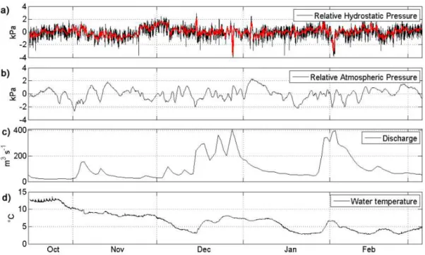
During the study period from 16 October 2012 to 6 March 2013, the average daily discharge ranged from 18.5 to 405 m3s−1 (Fremersdorf gauging station), with an average of 109 m3s−1and a median of 63 m3s−1. Over 50 % of all days, the discharge was below 65 m3s−1. Three major flood peaks occurred from 2 to 13 November, 14 December to 8 January, and 28 January to 14 February (Fig. 3). Water tem-perature ranged between 2.8◦C and 13.5◦C (Fig. 3). From 16 to 27 October, diurnal thermal stratification occurred. The water column was well mixed during the rest of the study period.
Figure 3. (a) Relative hydrostatic (original data in black, low-frequency filtered in red), (b) atmospheric pressure, (c) discharge and (d) water temperature between 16 October 2012 and 6 March 2013.
0.74 m, while the standard deviation of the water level was 0.07 m (Fig. 3).
Analysis of the high-pass filtered hydrostatic pressure sig-nal of the LR-PS allowed one to distinguish periods with high and low pressure variability. The high-variability peri-ods were characterized by intensive ship locking activity that induced multiple surges (Maeck and Lorke, 2013), and cor-responding passages of ships were observed. The passage of a surge is characterized by a defined wave crest or trough over a period of ∼12 min, while the passage of a ship of-ten showed a strong (up to 30 cm of water level) but short (<1 min) decrease in pressure in the LR-PS signal. In the HR-PS measurements, ship waves could be discriminated from wind-induced surface waves by their short duration and due to their higher maximum wave amplitude. We chose a threshold of 2 cm for separation. Ship waves showed on av-erage a maximum wave height of 4.2 cm; however, they often reached maximum wave heights between 10 and 20 cm.
3.2 Characterization of ebullition
Deliberately released gas bubbles had CH4volume concen-trations between 48.6 % and 92.1 % with a mean of 80.5 %. For the conversion of the volume measurements with the ABTs to the ebullition rate, a concentration of 80 % CH4was used (Table 1). Gas concentrations of naturally released bub-bles are reported to vary strongly, but since we focus on the temporal dynamics in ebullition, we used the average con-centration of deliberately released bubbles for the flux esti-mates.
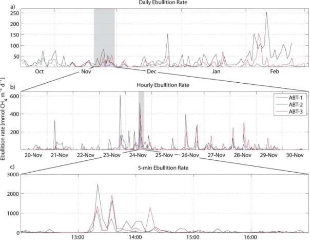
We observed high variability in the ebullitive flux on all temporal scales, ranging from minutes to days (Fig. 5). The daily ebullition rate ranged from 0 up to 240, 48 and 147 mmol CH4m−2d−1 for 1, 2 and ABT-3, respectively. The median daily ebullition rate for the entire sampling period was 22.4 (8.8/48.3, values repre-sent the 25th and 75th percentiles), 3.5 (0.6/8.0) and 9.1 (3.5/16.8) mmol CH4m−2d−1, at 1, 2 and ABT-3, respectively. From October to the end of January, the mean monthly ebullition rate showed no trend, while in February, the ebullition rate increased strongly for ABT-1 and ABT-3.
A significant difference in the ebullition rate between day- and night-time could be observed for all three ABTs (Wilcoxon test,pvalues are all below 0.05). On average, the daytime ebullition rates were 62 %, 42 % and 11 % higher compared to the nighttime ebullition rates for ABT-1, ABT-2 and ABT-3, respectively.
a)
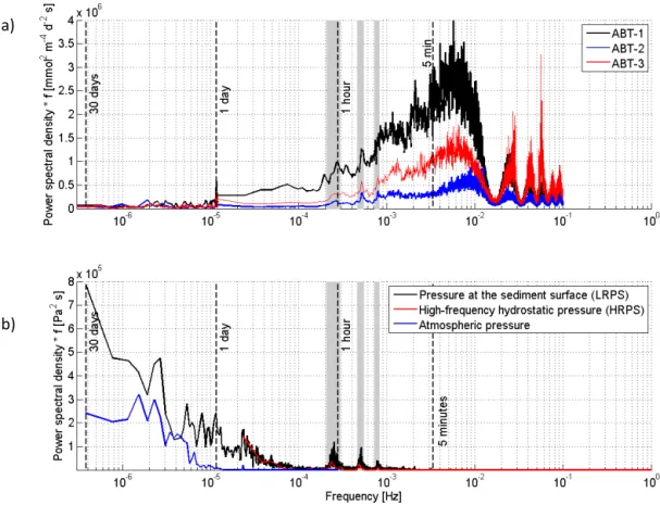
b)
Figure 4. Variance-preserving power spectra of ebullition rates (a) and hydrostatic (LR-PS and HR-PS) and atmospheric pressure in (b). Peaks at 15 min, 30 min and 1 h are marked in grey and caused by ship lock-induced surges.
Table 1. Monthly mean±SD and overall mean±SD concentrations of CH4in deliberately released and captured bubbles of the three automated bubble traps (ABTs) during the entire sampling period.
Nov Dec Jan Feb Mar Mean±SD per ABT
[% CH4] [% CH4] [% CH4] [% CH4] [% CH4] [% CH4]
ABT-1 89.8 81.1 48.6 71.1 89.5 76.0±17.1
ABT-2 89.2 80.9 76.6 78.0 88.5 82.6±5.9
ABT-3 89.5 84.2 72.8 75.0 92.1 82.7±8.6
Monthly mean±SD 89.5±0.3 82.1±1.8 66.0±15.2 74.7±3.5 90.0±1.9 80.5±10.2
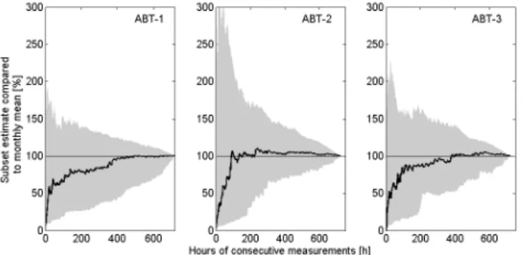
occurred frequently. Therefore, the best approach to achiev-ing a representative estimate of the monthly mean ebullition rate is to use longer measurement periods for the calculation. Figure 6 shows how the range between the 10th and 90th per-centiles of the subset mean ebullition rate is largest for sam-pling durations of only several hours and decreases with in-creasing measurement periods. Ultimately, there was an 80 % chance of estimating the 30-day mean ebullition rate with a precision of±50 % after measurements of consecutive 303, 375 or 280 hr for ABT-1, ABT-2 and ABT-3, respectively.
Ebullition occurred episodically, often in bursts of several bubbles entering the bubble trap indicated by the observation that the volume measured every 5 s often exceeded the ume of a typical bubble having a 5 mm diameter and a
vol-ume of∼0.5 ml (McGinnis et al., 2006). Not all but many bursts were synchronized between all three ABTs (Fig. 7). The cross-correlation between ABTs shows a distinct max-imum at zero lag, which indicates that a major portion of ebullition events are synchronized. Secondary small peaks were observed at a±1 h time lag, which corresponds to the re-occurrence of ship lock-induced surges after propagation along the entire impoundment, reflection and backward prop-agation (Maeck and Lorke, 2013).
3.3 Mechanisms triggering ebullition
Figure 5. Temporal variability of ebullition rates observed using the three automated bubble traps (ABTs) at different timescales: (a) Daily mean ebullition rates for the entire sampling period. (b) Hourly mean and (c) 5 min mean ebullition rates for selected time periods indicated by the grey bars in (a) and (b).
Table 2. Ebullition rates in mmol m−2d−1. All ebullition rates are shown as the median and 25th and 75th percentiles (in brackets). The day- and night-time ebullition rates refer to the hourly measured ebullition rates, while the daily ebullition rate is based on the daily ebullition rate. TheN,pvalues andzvalues represent the results of a Wilcoxon test comparing day- and night-time ebullition rates.
ABT-1 ABT-2 ABT-3
Daily ebullition rate 22.4 [8.8–48.3] 3.5 [0.6–8.0] 9.1 [3.5–16.8] Daytime ebullition rate (7 am–7 pm) 20.4 [10.1–62.2] 1.7 [0.6–7.3] 9.3 [3.6–20.9] Nighttime ebullition rate (7 pm–7 am) 12.6 [4.4–35.0] 1.2 [0.36–4.6] 3.7 [1.2–12.4] N,pvalue,zvalue 98,<0.01, 2.76 102, 0.04, 2.06 102,<0.01, 3.07
(corresponding to∼1 g CH4m−2d−1)revealed that 59.4 % of all investigated ebullition rates occurred during the pas-sage of a negative ship lock-induced surge (wave trough), 26.4 % during the passage of a ship, 5.7 % during periods of sinking water levels and 7.5 % during times where no pres-sure change was observed. Only one of the investigated ebul-lition events (0.9 %) was observed during the passage of a positive surge. The detailed temporal dynamics of ebullition rates in relation to the major forcing mechanisms are exem-plified in Fig. 8. The physical forcing of bubble release by surges and ship passages was the major regulator for the
tim-ing of ebullition. However, we also observed examples where no response of ebullition followed these forcing events.
Figure 6. Mean ebullition rates averaged over subsets of varying length representing consecutive measurement periods normalized by the mean ebullition rate observed over a 30-day period centered around the respective subset for the automated bubble traps (ABT 1 to 3) (left to right). The black line shows the median of all subsets and the grey area denotes the 10th and 90th percentiles.
variability periods (22, 4 and 8 mmol CH4m−2d−1for ABT-1, ABT-2 and ABT-3, respectively).
4 Discussion
4.1 Variability and magnitude of ebullitive emissions All sampling sites of this study are characterized by high sed-iment accumulation and high CH4concentrations and ebulli-tive release, which indicates high production rates of CH4 (Maeck et al., 2013). The trend that ebullition rates posi-tively correlate with sediment accumulation rates observed by Maeck et al. (2013) also holds true for the long-term mea-surements presented here. ABT-1 located over a site with the highest sediment accumulation rate (0.29 m yr−1, Fig. 1, de-termined following Maeck et al., 2013) showed the highest mean ebullition rate, followed by ABT-3 and ABT-2 with sediment accumulation rates of 0.1 and 0.07 m yr−1, respec-tively. Therefore, the CH4production rate per square meter likely differs between the three sites. If CH4production rates correlate with sedimentation rates, which is likely, then we observe that the variability in the daily ebullition rate also increased with production rate. However, it is likely that the ebullition variability was a factor in frequent forcing as well as production rate (Fig. 9).
The magnitude of CH4 ebullition rates measured in the present study are lower compared to the results of Maeck et al. (2013), where the ebullition rate was measured using hy-drostatics and correlated with the sediment accumulation rate (22.4 vs. 431, 9.1 vs. 14.4 and 3.5 vs. 8.4 mmol CH4m−2d−1 for ABT-1, ABT-2 and ABT-3, respectively), which may be the result of differing sediment temperatures. While the data presented here were measured during the winter when tem-peratures were low, the study by Maeck et al. (2013) was per-formed in September when water temperatures were higher. However, these current results are higher than total CH4
Figure 7. Cross-correlation coefficients of the 5 min ebullition rates versus the time lag of the three ABTs against each other. Peaks at zero lag indicate that both signals are synchronized.
emission rates reported for temperate lakes, rivers or reser-voirs (4, 0.9 and 1 mmol CH4m−2d−1, respectively) and comparable to emissions of tropical (<25◦ latitude) reser-voirs (16 mmol CH4m−2d−1, Bastviken et al., 2011; Varad-harajan and Hemond, 2012), as was also observed in a Swiss hydropower reservoir (DelSontro et al., 2010). The tempo-ral variability of ebullition rates was extremely high, as ob-served by Varadharajan and Hemond (2012); hence, for reli-able measurements of ebullitive emissions the temporal vari-ability must be considered in the planning stages of future studies.
Our results clearly show that ebullition is episodic, occur-ring in bursts consisting of many bubbles. The reason for this can be two-fold. On the one hand, external forcing (e.g., pres-sure reduction) can increase the volume of all bubbles within the sediment, from which a portion then has a buoyancy ex-ceeding the strength of the surrounding sediment and starts to rise (Boudreau et al., 2005). On the other hand, as soon as the first bubbles rise, they form conduits or rise tracks that make it easier for other bubbles to follow (Boudreau et al., 2005; Scandella et al., 2011). Besides external forcing, bubbles can also be released by ongoing CH4 production and continu-ous bubble growth and rise. This mechanism would lead to unsynchronized ebullition rates between sites and, when av-eraged over longer timescales, to constant flux rates that will then respond to changes in CH4productivity, e.g., due to tem-perature changes or changes in the amount of organic matter to be mineralized. The results of this study show, however, that anthropogenic mechanical forcing dominates the tempo-ral pattern of ebullition on timescales of days to weeks, not continuous CH4production.
Figure 8. Time series of 5 min ebullition rates and hydrostatic pressure changes. Panel (a) shows bubble release during sinking water level within a high-discharge period (25 December 2012). Panel (b) shows the relationship between positive and negative (grey shaded) surges and the ebullition rates (31 October 2012), while panel (c) highlights ebullition during the corresponding ship passages (grey shaded) (18 February 2013).
the groundwater, and to a lesser extent by microbial heat production associated with the degradation of organic mat-ter (Fang and Stefan, 1996; Fang and Stefan, 1998). Only the top layer of the sediment is strongly affected by heat ex-change with the overlying water column and therefore sub-ject to pronounced temperature variations, while the temper-ature variability decreases with increasing depth (Fang and Stefan, 1998). Since water temperatures were low, we as-sume that during our study period the production zone of CH4was mainly within deeper sediment layers, where the ef-fective temperature for methanogenesis changed only slowly compared to the timescale of forcing mechanisms. No direct relationship between water temperature and ebullition rate was observed, indicating that the temperature within the sed-iment responds only slowly to water temperature changes. The high degree of synchronization (Fig. 7) and the observa-tion that most of the gas was released during high-variability periods of hydrostatic pressure reveal the importance of the forcing regime for the temporal pattern of bubble release. In the case of the River Saar, physical forcing mechanisms con-trol the temporal dynamics of ebullition on short timescales.
4.2 Forcing mechanisms
The ebullition rates during the daytime were significantly higher compared with the nighttime ebullition rates. At the Saar, there is no illumination of the sediment and therefore no warming of the sediment except by direct heat exchange be-tween the water and sediment, and we recorded no daily pat-tern in the temperature except from 16 to 25 October 2012. Since temperatures within the sediment change over longer periods it can be assumed that there is only minor variation in the CH4production between day- and night-time caused by temperature changes. Hence, it is likely that there are other mechanisms that are responsible for the large temporal vari-ability in ebullition rates.
Figure 9. Conceptual framework for characterizing temporal vari-ability of ebullition in aquatic systems differing in the relation be-tween CH4production rates and forcing frequency of relevant trig-ger mechanisms for ebullition. All examples show ebullition rates (6-hour average) over a period of 4 weeks, except for (3), which refers to a period of 2 weeks. Example (1) shows the measured data from this study (Saar, ABT-1, January 2013), example (2) shows measurements from the Upper Mystic Lake (25 m site, Octo-ber) taken from Varadharajan et al. (2012) and example (3) shows measured data from the River Main, Germany (Krotzenburg Dam, September 2012).
changes can act as a trigger is consistent with the results of other studies (Chanton et al. 1989; Joyce and Jewell, 2003; Varadharajan and Hemond, 2012). However, not all pressure reductions, e.g., by negative surges, showed a response in the ebullition rate. This may be due to the history of bubble re-lease. If many bubbles were previously released the storage of free gas within the sediment may be smaller; therefore, even with an increase in gas volume due to pressure reduction the buoyancy of the gas may not be sufficient to cause bubble release. That the amount of free gas stored within a matrix can change was already shown for floating sediment mats in peatland (Fechner-Levy and Hemond, 1996) ship lock.
The passage of ships associated with different types of sur-face waves affected ebullition (Fig. 8c). However, ships can cause very different pressure changes and wave characteris-tics at the sampling site depending on the type of ship, its speed, the actual pathway of the ship track and the direction of the slipstream (Hofmann et al., 2008a). Therefore, the pas-sage of ships can but will not always trigger ebullition. The example shown in Fig. 8c demonstrates that several ship pas-sages had a strong effect on ebullition at ABT-1, but nearly no effect for the other two ABTs. This can result from the lo-cation of the ABTs and the morphology of the different sites.
While ships passed closer to ABT-1, ABT-2 and ABT-3 were further away from the main shipping channel and closer to the shore. Propagating diverging ship waves attenuate with travel length (Kundu and Cohen, 2008), but since ABT-2 and ABT-3 were closer than 80 m to the passing ships (ABT-1 is directly on the border of the shipping channel) the attenua-tion is of minor importance; therefore, the ship waves must have also been present at the locations of ABT-2 and ABT-3. Additionally, the shallower water depths at 2 and ABT-3 should have led to proportionally stronger pressure changes due to bypassing waves compared to ABT-1. The missing gas release at ABT-2 and ABT-3 indicates that at ABT-1 the ebullition was not triggered by diverging surface waves, but rather by other processes in the vicinity of the ship, e.g., draft-induced pressure changes. However, we observed vi-sually during our field campaigns that gas bubbles were re-leased massively following the passage of large ship waves, but only in the more shallow areas (< 2 m water depth). Since the pressure signal caused by surface waves decreases with increasing depth and decreasing wave length (Kundu and Co-hen, 2008), short waves, e.g., wind-induced or diverging ship waves, change the pressure at the sediment surface only in shallow regions, while long waves, e.g., surges, also affect the pressure in deeper areas.
Negative surges with a decrease in pressure showed stronger effects on ebullition compared to positive surges, which increase the pressure temporarily. Since the passage of both surges is associated with similar changes in current velocity (Maeck and Lorke, 2013), the effect of shear stress and pressure change on ebullition rates can be discriminated. Negative surges reduce the pressure, while positive surges in-crease the pressure. Significantly more large ebullition events co-occurred with negative surges, which indicates that the ef-fects of pressure changes were stronger compared to shear stress (Fig. 8b, results section).
Sinking water level can also be a trigger for bubble release (Fig. 8a), but in the case of the River Saar this effect was of minor importance. Temporal changes in storage height may be much more important for systems with strong changes in water level, e.g., caused by hydropower peaking (Zohary and Ostrovsky, 2011).
5 Implications
5.1 Timescale of forcing in other aquatic systems The temporal dynamics of forcing mechanisms can be ex-pected to differ among different aquatic systems. In lakes for example, water level changes are often caused by changes in the inflow of rivers on a timescale of days to weeks (Hof-mann et al., 2008b; Jöhnk et al., 2004; Wilcox et al., 2007). In large lakes that have sufficient fetch length for wind en-ergy input, seiches and propagating surface waves can gen-erate short-term pressure fluctuations (Hamblin and Hollan, 1978). In lakes with limited fetch length, atmospheric and hydrostatic pressure changes have been demonstrated to trig-ger ebullition rates (Varadharajan and Hemond, 2012). In reservoirs, the inflow of water and the operation of dams are important, since pressure is predominantly controlled by the water level. In these systems water level drawdown can trigger ebullition, but wind speed may also affect gas vent-ing (Joyce and Jewell, 2003). Ebullition rates in tidal sys-tems were shown to be controlled by the tidal rise and fall of the water level (Boles et al., 2001). In general, many inland waters are exposed to periodically occurring forcing mech-anisms with associated periods similar to those observed at the Saar.
The temporal pattern of ebullition from cohesive sedi-ments is governed by two major factors: the production rate of CH4(approximated here by using the sedimentation rate as a proxy) and the timescale of forcing of sufficient mag-nitude (Fig. 9) to release bubbles. Ultimately, the ratio be-tween the CH4 production rate and the forcing frequency is the parameter that controls the temporal pattern of ebul-lition. Short-term (high-frequency) forcing in combination with high CH4 production leads to the pattern observed within this study (Fig. 9-1) characterized by strongly variable ebullition rates on short timescales, but relatively constant fluxes after averaging over several days. Sites of lower CH4 production that experience long-term (low-frequency) forc-ing mechanisms will release bubbles mainly durforc-ing times of significant forcing, e.g., during water level reduction (Fig. 9-2), as observed by Varadharajan et al. (2012). Ultimately, the ratio of forcing frequency to CH4 production rate will be on the same order of magnitude for both examples (as seen in Fig. 9-1 and 9-2); therefore, the ebullition variabil-ity and the resulting temporal pattern are predominantly trolled by forcing mechanisms. In contrast to forcing con-trolled regimes, highly productive systems exposed to long-term forcing may release bubbles more consistently follow-ing the rate of CH4production al illustrated in Figs. 9-3 with data from another German impoundment (the River Main at the Krotzenburg dam) that were collected with the same instrumentation and analyzed with the same methods as in this study. This site was located on the side upstream of the dam, where no ships can pass by, and since the River Main has a much larger cross-sectional area and a higher
discharge, ship lock-induced surges will not significantly af-fect the hydrostatic pressure at this site. Therefore, the ebul-lition rate may vary only little, but enhanced ebulebul-lition can occur during strong forcing periods, e.g., during periods of decreasing atmospheric pressure. This is an example of a CH4production-controlled regime. To verify this conceptual framework, which provides a useful a priori estimate of the temporal variability of CH4 ebullition in aquatic systems, more high-resolution long-term ebullition data of different sites in combination with measurement of forcing parame-ters are necessary.
5.2 Implications for sampling intervals and duration The recently developed guidelines for measuring greenhouse gas emissions from reservoirs (UNESCO/IHA 2011) recom-mend performing ebullition measurements over a period of at least 24 hours. In the River Saar, we observed a daily pattern with higher fluxes during the day, when ship locking and ship traffic induce water level fluctuations. During the night when ship traffic decreased, the water level fluctuations decreased and the ebullition rate was lower. Therefore, it is necessary to sample day and night. However, since forcing can be of vary-ing magnitudes, the daily ebullition rate varied strongly and therefore, in the River Saar, ebullition measurements over 24 hours are not representative of longer periods (Fig. 6).
To determine the period of representative measurement, the variability in the ebullition rate itself is not the most im-portant factor but rather the time span between episodes of strong gas release (“bubbling episodes”). For accurate ex-trapolation of short-term measurements to longer periods, it is necessary to measure over periods that cover the timescale of the bubbling episodes several times, since there is variabil-ity between the episodes (Fig. 5) (Varadharajan and Hemond, 2012). A representative measurement period at the Saar has to cover more than 10 days (indicated by the median in Fig. 8). In aquatic systems with longer periods between bub-bling episodes, representative sampling periods will be much longer.
Our results show that short-term measurements are likely to underestimate the ebullition rate significantly, as illus-trated by the median flux in Fig. 6 consistently remaining be-low 50 % of the monthly mean flux at shorter timescales. In contrast, if measurements are mainly performed during day time, ebullition rates are likely to be overestimated because some forcing mechanisms, whether naturally occurring such as wind or anthropogenically induced such as ship waves, are more likely to occur during the day. If measurements are per-formed during randomly chosen periods of 24 hr or shorter, the chance to underestimate ebullition rates by over 50 % is large (an average median of 54 % underestimation at 24 hr in Fig. 6).
in systems with strong anthropogenic pressure changes like navigation channels, the interval should be at least 10 days, and for systems where natural forcing dominates, ebullition should be measured continuously because the timescale of atmospheric hydrostatic pressure changes is longer. Inves-tigating hydrostatic pressure changes will help to identify the forcing timescale at work. Shorter sampling intervals are likely representative in systems with CH4production and mi-nor physical forcing, but further studies are needed to support this.
Acknowledgements. The authors would like to thank the Water and
Shipping Agency of Saarbrücken (WSV) for their great support during the deployment of the ABTs and Helmut Fischer from the Federal Institute of Hydrology (BfG) for providing infrastructure and administrative support. Special thanks go to Florian Mäck, who developed the electronic part and the software interface of the ABTs, and to Sebastian Geissler, who constructed the housing and for his support during the field campaigns. We would like to thank the team of Lothar Laake of the workshop of the University of Göttingen for manufacturing the housing and Dan McGinnis and Tonya DelSontro for sharing the mechanical construction of the ABTs. We also thank three anonymous reviewers and the editor for their comments that helped to improve the manuscript. This study was financially supported by the German Research Foundation (grant LO 1150/5-1).
Edited by: T. Del Sontro
References
Bastviken, D., Tranvik, L. J., Downing, J. A., Crill, P. M., and Enrich-Prast, A.: Freshwater methane emissions offset the continental carbon sink, Science, 331, 50, doi:10.1126/science.1196808, 2011.
Baulch, H. M., Dillon, P. J., Maranger, R., and Schiff, S. L.: Dif-fusive and ebullitive transport of methane and nitrous oxide from streams: are bubble-mediated fluxes important?, J. Geo-phys. Res.-Biogeo., 116, doi:10.1029/2011JG001656, 2011. Becker, A., Kirchesch, V., Baumert, H. Z., Fischer, H., and
Schöl, A.: Modelling the effects of thermal stratification on the oxygen budget of an impounded river, River Res. Appl., 26, 572– 588, doi:10.1002/rra.1260, 2010.
Boles, J., Clark, J., Leifer, I., and Washburn, L.: Temporal varia-tion in natural methane seep rate due to tides, Coal Oil Point area, California, J. Geophys. Res.-Oceans, 106, 27077–27086, doi:10.1029/2000JC000774, 2001.
Boudreau, B. P., Algar, C., Johnson, B. D., Croudace, I., Reed, A., Furukawa, Y., Dorgan, K. M., Jumars, P. A., Grader, A. S., and Gardiner, B. S.: Bubble growth and rise in soft sediments, Geol-ogy, 33, 517–520, doi:10.1130/G21259.1, 2005.
Chanton, J. P., Martens, C. S., and Kelley, C. A.: Gas transport from methane-saturated, tidal freshwater and wetland sediments, Lim-nol. Oceanogr., 34, 807–819, 1989.
Coulthard, T., Baird, A., Ramirez, J., and Waddington, J.: Methane dynamics in peat: importance of shallow peats and a novel
reduced-complexity approach for modeling ebullition, carbon cycling in Northern Peatlands, Geophys. Monogr. Ser, 184, 173– 185, doi:10.1029/2008GM000811, 2009.
DelSontro, T., McGinnis, D. F., Sobek, S., Ostrovsky, I., and Wehrli, B.: Extreme methane emissions from a Swiss hy-dropower reservoir: contribution from bubbling sediments, En-viron. Sci. Technol., 44, 2419–2425, doi:10.1021/es9031369, 2010.
DelSontro, T., Kunz, M. J., Kempter, T., Wüest, A., Wehrli, B., and Senn, D. B.: Spatial heterogeneity of methane ebullition in a large tropical reservoir, Environ. Sci. Technol., 45, 9866–9873, doi:10.1021/es2005545, 2011.
Duc, N. T., Crill, P., and Bastviken, D.: Implications of temper-ature and sediment characteristics on methane formation and oxidation in lake sediments, Biogeochemistry, 100, 185–196, doi:10.1007/s10533-010-9415-8, 2010.
Emery, W. J. and Thomson, R. E.: Data Analysis Methods in Phys-ical Oceanography, Elsevier Science Limited, Amsterdam, the Netherlands, 2001.
Fang, X. and Stefan, H. G.: Dynamics of heat exchange between sediment and water in a lake, Water Resour. Res., 32, 1719–1727, 1996.
Fang, X. and Stefan, H. G.: Temperature variability in lake sediments, Water Resour. Res., 34, 717–729, doi:10.1029/96WR00274, 1998.
Fechner-Levy, E. and Hemond, H.: Trapped methane volume and potential effects on methane ebullition in a northern peatland, Limnol. Oceanogr., 41, 1375–1383, 1996.
Forster, P., Ramaswamy, V., Artaxo, P., Berntsen, T., Betts, R., Fa-hey, D. W., Haywood, J., Lean, J., Lowe, D. C., Myhre, G., Nganga, J., Prinn, R., Raga, G., Schulz, M., and Van Dorland, R.: Changes in Atmospheric Constituents and in Radiative Forcing, in: Climate Change, The Physical Science Basis, Contribution of Working Group I to the Fourth Assessment Report of the In-tergovernmental Panel on Climate Change, edited by: Solomon, S., Qin, D., Manning, M., Chen, Z., Marquis, M., Averyt, K. B., Tignor, M., and Miller, H. L., Cambridge University Press, Cam-bridge, United Kingdom and New York, NY, USA, 2007. Goodrich, J. P., Varner, R. K., Frolking, S., Duncan, B. N., and
Crill, P. M.: High-frequency measurements of methane ebulli-tion over a growing season at a temperate peatland site, Geophys. Res. Lett., 38, doi:10.1029/2011GL046915, 2011.
Hamblin, P. F. and Hollan, E.: On the gravitational seiches of Lake Constance and their generation, Schweiz. Z. Hydrol., 40, 119– 154, doi:10.1007/BF02502376, 1978.
Hofmann, H., Lorke, A., and Peeters, F.: The relative importance of wind and ship waves in the littoral zone of a large lake, Limnol. Oceanogr., 53, 368, doi:10.4319/lo.2008.53.1.0368, 2008a. Hofmann, H., Lorke, A., and Peeters, F.: Temporal and spatial scales
of water level fluctuations in lakes and their ecological implica-tions, Hydrobiol., 613, 85–96, doi:10.1007/s10750-008-9474-1, 2008b.
Hofmann, H., Federwisch, L., and Peeters, F.: Wave-induced release of methane: littoral zones as a source of methane in lakes, Lim-nol. Oceanogr., 55, 1990–2000, doi:10.4319/lo.2010.55.5.1990, 2010.
flood, Limnologica-Ecology and Management of Inland Waters, 34, 15–21, doi:10.1016/S0075-9511(04)80017-3, 2004. Johnson, B. D., Boudreau, B. P., Gardiner, B. S., and Maass, R.:
Mechanical response of sediments to bubble growth, Mar. Geol., 187, 347–363, doi:10.1016/S0025-3227(02)00383-3, 2002. Joyce, J. and Jewell, P. W.: Physical controls on methane ebullition
from reservoirs and lakes, Environ. Eng. Geosci., 9, 167–178, doi:10.2113/9.2.167, 2003.
Kiene, R. P.: Production and consumption of methane in aquatic systems. Microbial production and consumption of greenhouse gases: Methane, nitrogen oxides and halomethanes, American Society for Microbiology, 111–146, 1991.
Kundu, P. K. and Cohen, I. M.: Fluid Mechanics, 4th edn., Elsevier Academic Press, Burlington, USA, 2008.
Leifer, I. and Patro, R. K.: The bubble mechanism for methane transport from the shallow sea bed to the surface: a re-view and sensitivity study, Cont. Shelf Res., 22, 2409–2428, doi:10.1016/S0278-4343(02)00065-1, 2002.
Liikanen, A. and Martikainen, P. J.: Effect of ammonium and oxy-gen on methane and nitrous oxide fluxes across sediment–water interface in a eutrophic lake, Chemosphere, 52, 1287–1293, doi:10.1016/S0045-6535(03)00224-8, 2003.
Lorke, A., McGinnis, D. F., Maeck, A., and Fischer, H.: Effects of ship locking on sediment oxygen uptake in impounded rivers, Water Resour. Res., 48, WR012514, doi:10.1029/2012WR012483, 2012.
Maeck, A. and Lorke, A.: Ship-lock induced surges in an im-pounded river and their impact on subdaily flow velocity vari-ation, River Res. Appl., doi:10.1002/rra.2648, 2013.
Maeck, A., DelSontro, T., McGinnis, D. F., Fischer, H., Flury, S., Schmidt, M., Fietzek, P., and Lorke, A.: Sediment trapping by dams creates methane emission hot spots, Environ. Sci. Technol., 47, 8130–8137, doi:10.1021/es4003907, 2013.
McGinnis, D., Greinert, J., Artemov, Y., Beaubien, S., and Wüest, A.: Fate of rising methane bubbles in stratified waters: how much methane reaches the atmosphere?, J. Geophys. Res.-Oceans, 111, C09007, 8130–8137, doi:10.1029/2005JC003183, 2006.
Scandella, B. P., Varadharajan, C., Hemond, H. F., Ruppel, C. and Juanes, R.: A conduit dilation model of methane vent-ing from lake sediments, Geophys. Res. Lett., 38, L06408, doi:10.1029/2011GL046768, 2011.
Schöl, A.: Die Saar – Auswirkungen der Stauregelung auf den Sauerstoffhaushalt in einem abflussarmen Mittelgebirgsfluss, in: Staugeregelte Flüsse in Deutschland, edited by: Kinzel-bach, F. G., Ragnar, Stuttgart, Germany, 2006.
Segers, R.: Methane production and methane consumption: a review of processes underlying wetland methane fluxes, Biogeochem-istry, 41, 23–51, doi:10.1023/A:1005929032764, 1998. Sobek, S., DelSontro, T., Wongfun, N., and Wehrli, B.:
Ex-treme organic carbon burial fuels intense methane bubbling in a temperate reservoir, Geophys. Res. Lett., 39, L01401, doi:10.1029/2011GL050144, 2012.
UNESCO/IHA: GHG Measurement Guidelines for Freshwater Reservoirs, edited by: Goldenfum, J. A., UNESCO, IHA, 2010. USACE: Hydaulic design – surges in canals – change 1, in:
Engi-neering and Design, US Army Corps of EngiEngi-neering, Washing-ton, DC, USA, 1–15, 1949.
Varadharajan C., Hermosillo R., and Hemond H. F.: A low-cost au-tomated trap to measure bubbling gas fluxes, Limnol. Oceanogr. Meth., 8, 363–375, doi:10.4319/lom.2010.8.363, 2010
Varadharajan, C. and Hemond, H. F.: Time-series analy-sis of high-resolution ebullition fluxes from a stratified, freshwater lake, J. Geophys. Res.-Biogeo., 117, G02004, doi:10.1029/2011JG001866, 2012.
Venkiteswaran, J. J., Schiff, S. L., St. Louis, V. L., Matthews, C. J., Boudreau, N. M., Joyce, E. M., Beaty, K. G., and Bo-daly, R. A.: Processes affecting greenhouse gas production in ex-perimental boreal reservoirs, Global Biogeochem. Cy., 27, 1–11, doi:10.1002/gbc.20046, 2013.
Wik M., Crill, P. M., Varner, R. K., and Bastviken, D.: Mul-tiyear measurements of ebullitive methane flux from three subarctic lakes, J. Geophys. Res. Biogeo., 118, 1307–1321, doi:10.1002/jgrg.20103, 2013
Wilcox, D. A., Thompson, T. A., Booth, R. K., and Nicholas, J.: Lake-level variability and water availability in the Great Lakes, US Geological Survey, 2007.