Biogeosciences, 10, 6677–6698, 2013 www.biogeosciences.net/10/6677/2013/ doi:10.5194/bg-10-6677-2013
© Author(s) 2013. CC Attribution 3.0 License.
Biogeosciences
Open Access
Indian Ocean Dipole and El Niño/Southern Oscillation impacts on
regional chlorophyll anomalies in the Indian Ocean
J. C. Currie1,2, M. Lengaigne3, J. Vialard3, D. M. Kaplan4, O. Aumont5, S. W. A. Naqvi6, and O. Maury4,7
1Biological Sciences Department, Marine Research Institute, University of Cape Town, Cape Town, South Africa 2Egagasini Offshore Node, South African Environmental Observation Network, Cape Town, South Africa
3Institut de Recherche pour le Développement, Laboratoire d’Océanographie et du Climat: Expérimentation et Approches
Numériques, UMR 7617, Université Pierre et Marie Curie, Paris, France
4Institut de Recherche pour le Développement, UMR212 EME (IRD, IFREMER, Université Montpellier II), Sète cedex,
France
5Institut de Recherche pour le Développement, Laboratoire de Physique des Océans, UMR6523, Brest, France 6CSIR-National Institute of Oceanography, Dona Paula, Goa, India
7Department of Oceanography, Marine Research Institute, University of Cape Town, Cape Town, South Africa
Correspondence to:J. C. Currie (jockcurrie@gmail.com)
Received: 25 February 2013 – Published in Biogeosciences Discuss.: 26 March 2013 Revised: 3 September 2013 – Accepted: 4 September 2013 – Published: 24 October 2013
Abstract. The Indian Ocean Dipole (IOD) and the El Niño/Southern Oscillation (ENSO) are independent climate modes, which frequently co-occur, driving significant inter-annual changes within the Indian Ocean. We use a four-decade hindcast from a coupled biophysical ocean general circulation model, to disentangle patterns of chlorophyll anomalies driven by these two climate modes. Comparisons with remotely sensed records show that the simulation com-petently reproduces the chlorophyll seasonal cycle, as well as open-ocean anomalies during the 1997/1998 ENSO and IOD event. Results suggest that anomalous surface and euphotic-layer chlorophyll blooms in the eastern equatorial Indian Ocean in fall, and southern Bay of Bengal in winter, are pri-marily related to IOD forcing. A negative influence of IOD on chlorophyll concentrations is shown in a region around the southern tip of India in fall. IOD also depresses depth-integrated chlorophyll in the 5–10◦S thermocline ridge
re-gion, yet the signal is negligible in surface chlorophyll. The only investigated region where ENSO has a greater influence on chlorophyll than does IOD, is in the Somalia upwelling re-gion, where it causes a decrease in fall and winter chlorophyll by reducing local upwelling winds. Yet unlike most other regions examined, the combined explanatory power of IOD and ENSO in predicting depth-integrated chlorophyll anoma-lies is relatively low in this region, suggestive that other
drivers are important there. We show that the chlorophyll impact of climate indices is frequently asymmetric, with a general tendency for larger positive than negative chloro-phyll anomalies. Our results suggest that ENSO and IOD cause significant and predictable regional re-organisation of chlorophyll via their influence on near-surface oceanogra-phy. Resolving the details of these effects should improve our understanding, and eventually gain predictability, of interan-nual changes in Indian Ocean productivity, fisheries, ecosys-tems and carbon budgets.
1 Introduction
(Wang and Fiedler, 2006). The SST expression of ENSO events generally peak between November and January (Tren-berth, 1997). Teleconnections associated with El Niño result in an overall warming of the Indian Ocean (Klein et al., 1999; Murtugudde and Busalacchi, 1999; Xie et al., 2009), due to changing cloud cover and wind patterns that relate to changes in ascending and descending branches of the Walker circu-lation (Du et al., 2009; Reason et al., 2000; Venzke et al., 2000). In turn, such physical perturbations can affect the biol-ogy in local and distant oceans (Ménard et al., 2007; Spencer et al., 2000; Vinueza et al., 2006). Applying empirical or-thogonal function (EOF) analyses to 4 yr of global SeaW-iFS data, which provide an estimate of surface phytoplank-ton biomass, Yoder and Kennelly (2003) identified two in-terannual modes of variability in surface chlorophyll, both of which they ascribed to ENSO control.
Whereas the Indian Ocean was previously considered to be largely passive to the interannual forcing of ENSO, it was shown in the late 1990s to exhibit its own mode of inter-annual variability (Murtugudde and Busalacchi, 1999; Saji et al., 1999; Webster et al., 1999), which impacts both lo-cal and remote regions (Izumo et al., 2010; Yamagata et al., 2004). This mode is commonly referred to as the Indian Ocean Dipole (IOD) mode, even though contention exists over whether it should be referred to as a ‘dipole’ (Baquero-Bernal et al., 2002; Hastenrath, 2002). A positive event is associated with anomalous easterly winds in the central In-dian Ocean and cold SST anomalies off the south and west coasts of Java and Sumatra. These two anomalies enhance each other in a positive feedback loop (Reverdin et al., 1986; Webster et al., 1999) similar to the Bjerknes feedback critical to ENSO events (Bjerknes, 1969). The anomalous easterly winds raise the thermocline in the eastern part of the basin and, together with off-equatorial Rossby wave responses, deepen the thermocline and warm the SST in the western Indian Ocean, resulting in characteristic zonal anomaly pat-terns in sea level height, as well as surface and subsurface temperature structures (e.g. Feng and Meyers, 2003; Mur-tugudde et al., 2004; Rao et al., 2002). Thermocline anoma-lies typically initiate earlier and persist longer than the sur-face temperature signals (Horii et al., 2008). Negative IOD events feature opposite anomalies over similar regions (Mey-ers et al., 2007; Vinayachandran et al., 2002). Like ENSO, IOD events are phase-locked to the seasonal cycle and velop during boreal spring, peak in about October, and de-cay by the end of the calendar year. IOD events are com-monly triggered by El Niño events and frequently co-occur with them, yet they also occur independently and thus are considered an independent climate mode (Annamalai et al., 2003; Meyers et al., 2007; Song et al., 2007; Yamagata et al., 2004).
Compared to the impacts on the physical structure of the Indian Ocean, the biological consequences of IOD events have received far less attention, despite their potential impor-tance to ecosystems, fishery resources and carbon
sequestra-tion. After the launch of SeaWiFS and with recent progres-sion of coupled biophysical ocean models, the fields required to investigate seasonal and interannual variability at basin scales have become increasingly accessible (e.g. Rodgers et al., 2008; Wiggert et al., 2005, 2006, 2009; Yoder and Kennelly, 2003). Satellite coverage of chlorophyll concentra-tions has allowed investigation of the most recent ENSO/IOD events (e.g. Iskandar et al., 2009; Murtugudde et al., 1999; Wiggert et al., 2009). The intense 1997 positive IOD/El Niño event was characterised by a strong phytoplankton bloom in the eastern equatorial Indian Ocean; an area which is nor-mally characterised by low productivity (Murtugudde et al., 1999; Susanto and Marra, 2005). The upwelling of cool, nutrient-rich water and associated biological productivity had a detrimental impact on coral reefs in a large area off the coast of Indonesia (Abram et al., 2003, 2004; van Woe-sik, 2004). Other documented impacts of the 1997 event in-cluded a decrease of surface chlorophyll in the Arabian Sea (Sarma, 2006) attributed to anomalous northeasterly winds, as well as a bloom in the southeastern Bay of Bengal, owing to anomalous Ekman pumping in this region (Vinayachan-dran and Mathew, 2003). Although similar blooms developed in the eastern Indian Ocean during the 2006 IOD (Iskandar et al., 2009), Wiggert et al. (2009) showed that the biological re-sponses to the 1997 event were of greater intensity, with more persistent and stronger positive anomalies spreading further west than in 2006, due to a reversal (as opposed to weaken-ing) of the Wyrtki jet in the boreal fall intermonsoon. In ad-dition, their results showed that the bloom in the southeast-ern Bay of Bengal and the low chlorophyll anomaly in the Arabian Sea observed during 1997 developed only weakly during the less severe 2006 event.
Wiggert et al. (2009) made use of a remote sensing-based algorithm to make a first assessment of basin-wide primary production (NPP) anomalies caused by the 1997 and 2006 IOD/El Niño events. These events appeared to have had a minimal effect on the net NPP averaged over the event peri-ods and entire Indian Ocean, due to compensating responses among different regions. There is however a profound redis-tribution of the carbon uptake, with a large NPP increase in the eastern Indian Ocean, roughly balanced by a decrease in western regions. While the two events did not signifi-cantly impact surface chlorophyll in the southwestern In-dian Ocean, the region did exhibit negative NPP anomalies, due to anomalously deep thermocline depths (Wiggert et al., 2009). NPP anomalies varied considerably, depending on the event considered: positive NPP anomalies in the eastern In-dian Ocean varied between 45 and 13 %; negative anomalies in the southwestern Indian Ocean varied between−20 and −8 %; while the Arabian Sea experienced NPP changes of −9 and +15 % during the 1997 and 2006 events respectively.
These contrasts reveal the changing nature of biological im-pacts among different events.
J. C. Currie et al.: IOD and ENSO impacts on Indian Ocean chlorophyll 6679
restrictive in addressing interannual or long-term changes. Only two clear positive IODs have developed during the SeaWiFS era, which represents a limited sample size and does not allow investigation of the full spectrum of pos-sible IOD/ENSO configurations (e.g. Meyers et al., 2007; Song et al., 2008). Moreover, problems with remotely sensed chlorophyll in some oligotrophic regions have been noted (Claustre et al., 2002; Dandonneau et al., 2003) and sen-sors potentially miss a proportion of depth-integrated chloro-phyll when chlorochloro-phyll maxima are deeper than the first op-tical depth or “penetration depth” (∼20 m; Gordon and
Mc-Cluney, 1975). Fortunately, longer-term biogeochemical and biological hindcasts from coupled biophysical models are increasingly capable of revealing subsurface processes not captured by satellites, and are resolving seasonal and inter-annual variability to an ever-improving degree (e.g. Koné et al., 2009; Maury, 2010; Rodgers et al., 2008; Wiggert et al., 2006).
This study aims to investigate the interannual changes in chlorophyll caused by IOD- and ENSO-induced changes to the physical ocean. We make use of a four-decade hind-cast from the coupled biophysical general circulation model, NEMO-PISCES, to separate the respective contributions of ENSO and IOD to surface and vertically integrated chloro-phyll anomalies in the Indian Ocean. Focusing predomi-nantly on the biological response, we also assess responses in SST, thermocline depth and surface winds to explore the physical processes driving the variability in chlorophyll. An improved understanding of such dynamics will aid construc-tive hypotheses about, and interpretations of, ecosystem links to climate variability and thereby contribute towards attain-ing predictability of impacts from similar events in future.
The paper is structured as follows. Section 2 describes the data and methods used. A brief comparison between the modelled surface chlorophyll and SeaWiFS outputs is pro-vided for the Indian Ocean in Sect. 3. Section 4 describes the influences of IOD and ENSO on thermal and chlorophyll responses in surface waters of the Indian Ocean. Section 5 summarises our main findings and discusses them in the con-text of relevant literature.
2 Data and methods
2.1 Observed data sets
Chlorophyll a (Chl a) concentrations were obtained from the European Space Agency’s GlobColour project. We used a remotely sensed level 3 (binned and mapped) 1◦ and
monthly resolution Chl a data set, which is derived using standard case 1 water algorithms (Morel and Maritorena, 2001; O’Reilly et al., 1998). This data set is a merged product from three sensors (SeaWiFS, MERIS, and MODIS-Aqua), which has approximately twice the mean global coverage and lower uncertainties in retrieved variables compared to
data from individual sensors (Maritorena et al., 2010). While small systematic differences exist among the products of in-dividual sensors, the large-scale Chladistributions produced by these major ocean colour missions are consistent over a wide range of conditions (Djavidnia et al., 2010; Morel et al., 2007).
2.2 Ocean model and forcing data sets
Hindcasts from an ocean general circulation model (OGCM), coupled to a biogeochemical model were used to investi-gate interannual anomalies of chlorophyll and physical vari-ables. The simulation used in this paper has been detailed in Koné et al. (2009), so we describe only its main features here. The NEMO ocean configuration was built from the OPA (Ocean PArallelise) version 8.2 ocean model (Madec et al., 1998), coupled to the dynamic-thermodynamic Louvain-la-Neuve sea ice model (LIM; Timmermann et al., 2005). This 0.5◦configuration (known as ORCA05-LIM; cell size ∼50 km in the tropics) has 30 vertical levels, of which 20
are concentrated in the upper 500 m; their thickness increas-ing from 10 m near the surface to 500 m at depth. Density was computed from potential temperature, salinity and pres-sure using the equation of state by Jackett and Mcdougall (1995). Vertical mixing was parameterised from a turbulence closure scheme based on a prognostic vertical turbulent ki-netic equation, which has been shown to perform well in the tropics (Blanke and Delecluse, 1993). Simulated lateral mix-ing acts along isopycnal surfaces, with a Laplacian opera-tor and 200 m2s−1 constant isopycnal diffusion coefficient
(Lengaigne et al., 2003). Penetration of short-wave fluxes into the ocean was based on a single exponential profile (Paulson and Simpson, 1977), corresponding to oligotrophic water (attenuation depth of 23 m). No-slip boundary condi-tions were applied at the coastlines.
The OGCM has been used extensively in an uncoupled mode (Cravatte et al., 2007; Lengaigne et al., 2002) and cou-pled with an atmospheric model (Lengaigne et al., 2006; Lengaigne and Vecchi, 2010), using various forcing strate-gies. It has been shown to accurately simulate the vertical structure of equatorial temperature and currents (Vialard et al., 2001), as well as the interannual variations of heat con-tent in the Pacific Ocean (Lengaigne et al., 2012). In addition, the model compared well with interannual sea level data from satellite altimetry and tide gauges in the tropical Indian and Pacific oceans (Nidheesh et al., 2012). Keerthi et al. (2013) show that the model simulates interannual variability of the mixed layer depth relatively well in the Indian Ocean, with similar spatial patterns and reasonable phase agreement com-pared to estimates from in situ data.
and brief validation of results is available in the supplemen-tary material of Aumont and Bopp (2006). The biogeochem-ical model has 24 compartments, which include two sizes of sinking particles and four “living” biological pools, rep-resented by two phytoplankton (nano-phytoplankton and di-atoms) and two zooplankton (microzooplankton and meso-zooplankton) size classes. Phytoplankton growth is limited by five nutrients: NO3, NH4, PO4, SiO4, and Fe. The ratios
among C, N, and P are kept constant for the “living” compart-ments, at values proposed by Takahashi et al. (1985). The in-ternal Fe contents of both phytoplankton groups and Si con-tents of diatoms are prognostically simulated as a function of ambient concentrations in nutrients and light level. De-tails on the red-green-blue model by which light penetration profiles are calculated, are given in Lengaigne et al. (2007). The Chl / C ratio is modelled using a modified version of the photo-adaptation model by Geider et al. (1998). Ratios of el-ements within zooplankton compartments are kept constant. Manuals for NEMO and PISCES are available online (http: //www.nemo-ocean.eu/About-NEMO/Reference-manuals).
The physical model was initialised from rest with salin-ity and temperature climatologies of the World Ocean At-las 2001 (Boyer et al., 2005). The biogeochemical model was initialised from outputs of the simulation described by Aumont and Bopp (2006). Thereafter a 7 yr spin-up period was performed on the coupled model and the simulation was run over the period 1958–2001. Surface boundary conditions were applied to the OGCM as follows: daily surface wind stresses were specified from the ERA40 re-analysis (Uppala et al., 2005). Radiation fluxes were based on the CORE v1 data set, using the International Satellite Cloud Climatol-ogy Project’s radiation product (Zhang et al., 2004), avail-able from 1984 onwards. Prior to 1984 a climatology of the radiation fluxes was imposed, which leads to better results than the use of reanalysis data. Precipitation was taken from the Climate Prediction Center Merged Analysis of Precipi-tation (CMAP; Xie and Arkin, 1997), available from 1979 onwards, while a CMAP climatology was applied before then. Evaporation and turbulent heat fluxes were computed using empirical bulk formulae by Goosse (1997), which em-ployed ERA40 daily wind speed and air temperatures, as well as climatological relative humidity fields from Trenberth et al. (1989). To avoid artificial model drift, sea surface salin-ity was restored towards monthly mean climatological val-ues from the World Ocean Atlas (Boyer et al., 2005), with a timescale of 300 days for a typical 50 m-thick mixed layer. Outputs were generated on a temporal resolution of 5 days.
Using the same model, Koné et al. (2009) show that In-dian Ocean features of the seasonal chlorophyll cycle com-pare reasonably well with SeaWiFS, including the timing of bloom onsets. In addition, recognised biogeochemical provinces are reproduced in most of the Arabian Sea, Bay of Bengal and in the convergence zone south of the Equator (Koné et al., 2009). In our analyses, the first 3 yr of the
simu-lation (1958–1960) were omitted, in order to avoid potential spin-up effects.
2.3 Methodology
The depth of the 20◦C isotherm (D20) was estimated by
linear interpolation of temperature between model levels. Chlorophyll concentrations were calculated as the sum of chlorophyll from the two phytoplankton size classes (di-atoms and nano-phytoplankton). Surface chlorophyll con-centrations (denoted bySChl; units of mg m−3)were
aver-aged over the upper two layers (i.e. 20 m depth) for compar-ison with SeaWiFS. The euphotic zone was estimated from the photosynthetically available radiation (PAR) outputs, as the depth where PAR was 1 % of the surface value. The depth-integrated chlorophyll was then computed over the eu-photic zone, and is referred to as integrated chlorophyll or IChl hereafter (units of mg m−2).
Interannual anomalies for all fields were computed from monthly time series as the remainder after removal of their mean seasonal cycle and “long-term trend” components by the seasonal decomposition of time series by loess func-tion (STL; Cleveland et al., 1990), in R programming lan-guage (R Development Core Team, 2011). The trend com-ponent was estimated by a degree-one polynomial fitted over a 7 yr loess window and serves to remove longer-term variability on the order of decades or greater. All analyses were performed on these anomalies, except for the seasonal comparison of average surface chlorophyll between model and SeaWiFS (Fig. 1). To represent the interannual sig-nals associated with IOD and ENSO, standard indices were used: the Pacific ENSO signal was represented by averaged SST anomalies over the Niño3.4 region during November– January (Trenberth, 1997). The IOD was characterised by the dipole mode index (DMI), computed as the difference between SST anomalies in the western and eastern equato-rial Indian Ocean during September–November (Saji et al., 1999). Both climate indices were standardised to unit vari-ance. The geographical limits used for calculation of the cli-mate indices are summarised in Table 1. Geographical re-gions in which the physical and biological variability was in-vestigated in more detail are also listed in Table 1 and shown in Figs. 3 and 6.
One of the principal objectives of this study was to sepa-rate the impacts of ENSO and IOD on Indian Ocean chloro-phyll and physical variables. Because of the frequent co-occurrence of IOD and ENSO events and the resultant corre-lation between their indices (∼0.53; Yamagata et al., 2004),
J. C. Currie et al.: IOD and ENSO impacts on Indian Ocean chlorophyll 6681
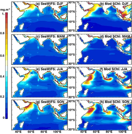
Fig. 1.Seasonal evolution of averageSChl patterns from SeaWiFS satellite estimates (left panels) and model outputs (right panels). Seasons are represented as December–February (DJF), March–May (MAM), June–August (JJA) and September–November (SON). The seasonal cycle was calculated over the 1998–2009 period for observations and 1990–2001 for the model (see Sect. 3 for details).
Table 1.Description and coordinate boundaries of the areas used in the calculation of climate indices and of regions investigated in greater detail. These regions of interest are also indicated in Figs. 3 and 6.
Abbreviation Description Latitudes Longitudes
Niño3.4 Niño3.4 region in the Pacific Ocean 5◦N–5◦S 120–170◦W
wDMI western Dipole Mode Index region 10◦N–10◦S 50–70◦E
eDMI eastern Dipole Mode Index region 0–10◦S 90–110◦E
EEIO eastern equatorial Indian Ocean; same as eDMI 0–10◦S 90–110◦E
wSCTR western Seychelles–Chagos thermocline ridge 5—15◦S 60–90◦E
SBoB southern Bay of Bengal 0–10◦N 85–100◦E
STI ocean around the southern tip of India 2–9◦N 70–85◦E
WAS western Arabian Sea 5–15◦N 50–63◦E
TIO tropical Indian Ocean 25◦N–25◦S 40–110◦E
on both. As an example, computation of the partial regres-sion between a time series of chlorophyll anomalies (CHL) and the IOD index (DMI), independently of the ENSO
in-dex (Niño3.4) required computation of three separate linear regressions:
DMI=b×Niño3.4+r.DMI−E, (2)
r.CHL−E=c×r.DMI−E+r.CHL−E−I. (3)
CHL and DMI were regressed on the Niño3.4 index (Eqs. 1, 2) to provide residuals that were free of linear ENSO signals (denoted r.CHL−E and r.DMI−E respectively). In a third
computation, these residuals were in turn regressed (Eq. 3) to provide an estimate of CHL variability that was linearly re-lated to IOD, without the effect of ENSO. The−Eand−I
sub-script notations indicate residuals that have had their ENSO or IOD signals removed respectively. Lettersa,bandc repre-sent regression coefficients that estimate the effect of the cli-mate indices on the chlorophyll anomalies (or clicli-mate index in Eqs. 2 and 5). A visual example of the removal of the linear climate mode signals from (in this case) CHL anomalies is provided in the supplementary material (Fig. S1). As climate indices (DMI and Niño3.4) were transformed to have zero mean and unit variance, these regression coefficients corre-spond to the change in the response variable (e.g. mg m−3
forSChl) that would be expected from a climate anomaly of magnitude 1.
The reciprocal partial regressions were also performed, removing the DMI signal from CHL (Eq. 4) and Niño3.4 (Eq. 5), before regressing their residuals to obtain an esti-mate of CHL variability that was related to ENSO without the effect of IOD (Eq. 6):
CHL=a×DMI+r.CHL−I, (4)
Niño3.4=b×DMI+r.Niño3.4−I, (5)
r.CHL−I=c×r.Niño3.4−I+r.CHL−I−E. (6)
Having removed the influence of DMI, the proportion of (in this case) CHL variance, explained purely by Niño3.4 (V.CHLNiño3.4), was estimated as the difference between
residual variances from Eqs. (4) and (6), relative to the vari-ance of the original CHL anomalies:
V .CHLNiño3.4=var(r.CHL−I)−var(r.CHL−I−E)
var(CHL) . (7)
Similarly, the variance explained purely by DMI was cal-culated as the difference between residual variances from Eqs. (1) and (3), relative to the variance of (in this case) CHL (not shown). Chlorophyll anomalies were substituted with D20 and SST anomalies in the above equations to com-pute the partial regressions for those variables respectively.
To complement the partial regression results, partial corre-lations between anomaly fields and DMI/ENSO indices were calculated as in Yamagata et al. (2004). When interpreting the results of partial regressions and partial correlations, one has to bear in mind that a proportion of joint variability, which is related to both IOD and ENSO, is removed from the result. Put differently, the explanatory power of “pure” IOD and “pure” ENSO signals from partial regressions will frequently add up to less than when they are combined in a multiple regression.
3 SeaWiFS and model comparison
Comparison of the model outputs and SeaWiFS is compli-cated by the fact that they overlap during a relatively short period of 4 yr (and 4 months). We chose to use a longer 10 yr period to provide a robust estimate of the seasonal clima-tology in our comparisons. These periods were selected to maximise the overlap between the model and observations: 1998–2009 for SeaWiFS and 1990–2001 for the model. Us-ing the common 1998–2001 period to estimate the climatol-ogy provided very similar results (not shown).
Estimates of surface chlorophyll from model outputs and SeaWiFS showed a similar picture overall, though the mag-nitude and spatial extent of simulated phytoplankton blooms are to some degree overestimated, while intense coastal blooms in SeaWiFS records are lacking in the model. Fig-ure 1 shows the mean seasonal cycle of surface chlorophyll in the model and observations. During the northeast mon-soon in boreal winter, elevatedSChl concentrations are found over the northwestern part of the Arabian Sea and the north-ern Bay of Bengal (BoB; Fig. 1a, b). Oligotrophic condi-tions prevail in the southeastern Arabian Sea, central BoB and in the Southern Hemisphere. These features are rela-tively well reproduced by the model, although the intensity of the bloom is overestimated along Somalia and around Sri Lanka (Fig. 1b). The spring intermonsoon is characterised for both model and observations by oligotrophic conditions and reduced chlorophyll in most of the Indian Ocean basin (Fig. 1c, d). During the summer/southwest monsoon and fall intermonsoon (Fig. 1e–h), the model correctly simulates phy-toplankton blooms along the coasts of Somalia and the Ara-bian Peninsula, at the southern tip of India, around Sri Lanka, along the Seychelles–Chagos thermocline ridge between 5 and 15◦S, and in the southeastern Indian Ocean. The
ampli-tude of these blooms is frequently overestimated in oceanic regions compared to SeaWiFS, whereas the chlorophyll val-ues are notably underestimated in the central Arabian Sea, resulting in an exaggerated gradient from the western conti-nental margin to the interior of the basin (Fig. 1e–h).
J. C. Currie et al.: IOD and ENSO impacts on Indian Ocean chlorophyll 6683
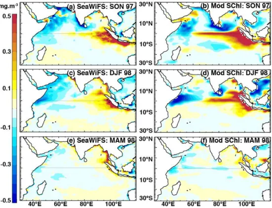
Fig. 2.Anomalies ofSChl during the 1997/1998 event from SeaWiFS satellite estimates (left panels) and model outputs (right panels). Anomalies were calculated with respect to a 1998–2009 climatology for SeaWiFS and a 1990–2001 climatology for the model (see Sect. 3 for details). Season abbreviations as in Fig. 1.
the model identified similar biogeographic provinces to Sea-WiFS data, specifically in most of the Arabian Sea, Bay of Bengal and in the convergence zone regions south of the Equator. These biogeochemical provinces were based on the cumulated increase in chlorophyll of summer or winter phy-toplankton blooms, as well as the timing of these bloom on-sets.
Anomalies during the 1997–1998 ENSO/positive IOD event display similar regional-scale features in SeaWiFS and the model (Fig. 2). The intense positive anomalies along the coastline of Sumatra and Java in fall were well simulated, al-though their intensity and westward equatorial extension are overestimated by the model (Fig. 2a, b). Positive anomalies persist throughout boreal winter in the eastern equatorial In-dian Ocean in both SeaWiFS and the model (Fig. 2c, d). The model correctly simulates a chlorophyll bloom in the south-eastern Bay of Bengal in winter (north of 4◦N and
extend-ing to 85◦E). In addition, the chlorophyll decrease along the
western coast and southern tip of India in fall is reasonably well captured by the model, although slightly overestimated in extent. The northern–central Arabian Sea shows some in-consistency between the model’s (positive) and SeaWiFS’ anomalies (negative) during the 1997/1998 winter season (Fig. 2c, d), indicative that the simulation may be lacking some dynamics in this area. However, the chlorophyll
de-creases in the western Arabian Sea in fall and their persis-tence along the Somalia coast in winter seem to be correctly predicted by the model.
4 Influence of IOD and ENSO in the Indian Ocean
4.1 Physical response
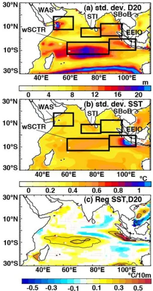
Investigation of surface temperature and thermocline depth anomalies provides an overview of regional variability in the physical response of the surface ocean to interannual forcing. Figure 3 highlights the regions of strong interannual vari-ability of the 20◦C isotherm depth (D20; a commonly used
proxy of thermocline depth in tropical waters) and SST. Re-gions of pronounced thermocline depth and SST variability include the Eastern Equatorial Indian Ocean (EEIO) and the western Seychelles–Chagos thermocline ridge between 5 and 10◦S (wSCTR). Changes in the shallow thermoclines seem
to influence SST to a large extent in these areas (Fig. 3c). Three additional regions chosen for further investigation in-clude areas of pronounced thermocline depth variability: the Southern Bay of Bengal (SBoB), Southern Tip of India (STI) and Western Arabian Sea (WAS).
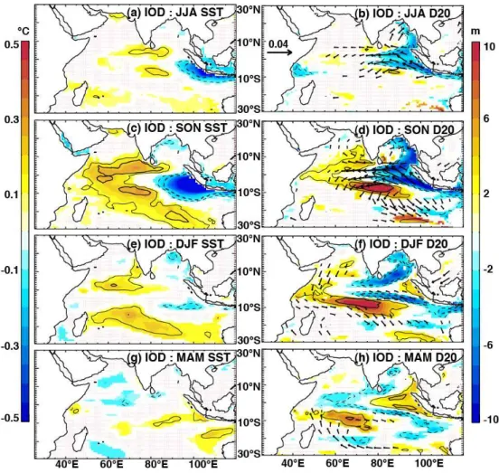
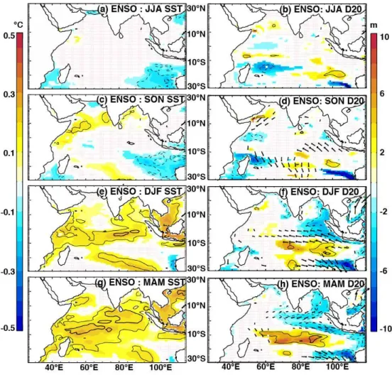
The partial regression methods allow us to separate statis-tically the anomaly signals that are related “purely” to one climate mode (e.g. IOD), having removed the linear signal of the other climate mode (e.g. ENSO). Because many of the surface temperature and thermocline depth responses to these climate modes have been detailed in the literature, we do not treat them comprehensively here and mainly focus on features relevant to chlorophyll anomalies. The physical re-sponse to positive IOD events is characterised by clear zonal gradients of SST and thermocline depth anomalies in the equatorial region, which peak in boreal fall (Fig. 4; Saji et al., 1999; Webster et al., 1999). The observed changes in ther-mocline depth are fuelled by surface wind anomalies (Fig. 4, right column): During boreal fall, a strong easterly anomaly arises near the Equator, which triggers an equatorial Kelvin wave response and generates upwelling in the eastern equa-torial region (Fig. 4b, d). The shoaling thermocline signal propagates as a coastal trapped Kelvin wave around the rim of the Bay of Bengal (in a counter-clockwise direction), as noted by Nidheesh et al. (2013) and Rao et al. (2010). An up-welling Rossby wave is reflected offshore (westwards) either side of the Equator, as illustrated by the two negative D20 lobes in Fig. 4b and d. Further west, the response is dom-inated by off-equatorial convergence due to Ekman pump-ing on the flanks of the equatorial easterly anomaly. The re-sult is a deeper-than-normal D20 in the central and western Indian Ocean, which propagates westwards as symmetrical Rossby wave signals either side of the Equator, from fall un-til the following spring (Fig. 4d, f, h). These deepened ther-mocline anomalies have a larger amplitude and are more per-sistent in the Southern Hemisphere, where they interact with the normally shallow Seychelles–Chagos thermocline ridge (Hermes and Reason, 2008; Yokoi et al., 2008).
The similarities in spatial patterns of D20 and SST anoma-lies, together with the regional relationships highlighted in Fig. 3c, suggest that thermocline depth variability is
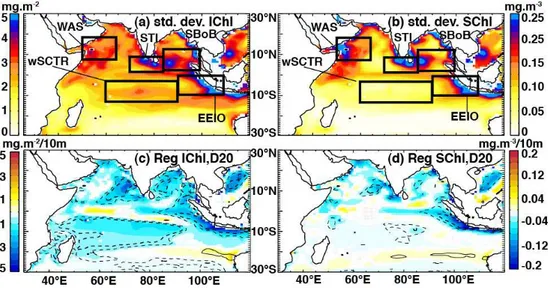
respon-Fig. 3.Regional interannual variance of(a)D20 and(b)SST, as in-dicated by the standard deviation of their anomalies over the period 1961–2001.(c)Coefficients from a simple linear regression of SST and D20 anomalies over the same period, drawn only when beyond a 90 % significance level. Thin and thick contours indicate corre-lation coefficients of 0.4 and 0.6 respectively, while solid (dashed) lines represent positive (negative) coefficients. Geographical boxes used in later analyses are shown in(a)and(b).
J. C. Currie et al.: IOD and ENSO impacts on Indian Ocean chlorophyll 6685
Fig. 4.The impacts of IOD on SST (left panels), D20 (colour; right panels) and wind stress (arrows; right panels), as indicated by partial regression coefficients of their anomalies regressed onto the IOD index, having removed the influence of ENSO (Eqs. 1–3). Regressions were computed for the period 1961–2001 and their coefficients were drawn only when beyond a 90 % significance level. Thin and thick contours indicate correlation coefficients of 0.4 and 0.6 respectively, while solid (dashed) lines represent positive (negative) correlations.
the distinct surface and subsurface impact of IOD and ENSO in the Indian Ocean (see also Rao and Behera, 2005; Yu et al., 2005). Whereas the IOD-related SST signal dissipates during winter, the basin-wide ENSO signal establishes during win-ter and peaks in spring (Klein et al., 1999; Xie et al., 2009), about 4–6 months after the mature phase of the IOD. Similar to IOD, ENSO-related anomalous equatorial easterly winds cause shallow D20 anomalies off Sumatra and in the east-ern Bay of Bengal, while concurrent deepening of the ther-mocline develops in the southern Indian Ocean in response to Ekman pumping (Fig. 5f). These ENSO anomalies are, however, delayed by at least a season compared to those of IOD and are less intense. The deep anomalies in the southern Indian Ocean propagate westwards during spring (Fig. 5h), consistent with a Rossby wave signal, but are weaker and centred further south than the corresponding IOD anomalies, congruent with the findings of Rao and Behera (2005) and Yu et al. (2005).
Even though ENSO does raise the thermocline near the eastern boundary in winter (Fig. 5f), strong upwelling-favourable winds that might lift these cooler waters to the surface (and thereby transfer the signal to SST) are likely stunted or precluded at this time of year by the monsoon-related wind reversal in the Northern Hemisphere (Schott et al., 2009; Xie et al., 2002).
4.2 Biological response
Fig. 5.The impacts of ENSO on SST (left panels), D20 (colour; right panels) and wind stress (arrows; right panels), as indicated by partial regression coefficients of their anomalies regressed onto the ENSO index, having removed the influence of IOD (Eqs. 4–6). Regressions were computed for the period 1961–2001 and their coefficients were drawn only when beyond a 90 % significance level. Thin and thick contours indicate correlation coefficients of 0.4 and 0.6 respectively, while solid (dashed) lines represent positive (negative) correlations.
EEIO. The wSCTR area shows marked variability in IChl (Fig. 6a), yet no corresponding signal inSChl (Fig. 6b).
Regression ofIChl on D20 reveals a significant negative relationship throughout most of the tropical Indian Ocean (Fig. 6c). Changes in thermocline depth control the proxim-ity of fertile subsurface waters to the sunlit euphotic zone and thereby affect phytoplankton productivity (Lewis et al., 1986; Messié and Chavez, 2012). The downwelling and re-sultant deep nutricline (thermocline) characteristic of ocean gyres means that horizontal advection of nutrients from ad-jacent regions can play a greater role in chlorophyll re-sponses there than vertical changes in the thermocline depth (McClain et al., 2004). This may explain the non-significant coefficients in the gyre regions west of Australia. Similarly, the central Arabian Sea is dominated by Ekman convergence in boreal summer (Schott et al., 2009), which together with strong coastal upwelling and offshore advection of nutrient-rich waters from the Somali and Oman coasts, might explain
the lack of a significant relationship in the western half of the Arabian Sea.
J. C. Currie et al.: IOD and ENSO impacts on Indian Ocean chlorophyll 6687
Fig. 6.Regional interannual variance of(a)IChl and(b)SChl, as indicated by the standard deviation of their anomalies over the period 1961– 2001.(c)Coefficients from a simple linear regression ofIChl and(d)SChl anomalies regressed onto D20 anomalies over the same period. Regression coefficients were drawn only when beyond a 90 % significance level. Thin and thick contours indicate correlation coefficients of 0.4 and 0.6 respectively, while solid (dashed) lines represent positive (negative) coefficients. Geographical boxes used in later analyses and selected on the basis of regional biogeochemical variability are shown in(a)and(b).
However, the simulation used here was forced with daily fields, therefore a diurnal effect would not explain the rela-tionship betweenSChl and D20 anomalies in our case. Be-yond those discussed above, most open-ocean regions reveal a weak or insignificant relationship betweenSChl and D20, indicative that factors beyond the vertical nutricline prox-imity play a greater role in controlling surface chlorophyll anomalies in these areas. The regions that display a signif-icantIChl–D20 relationship, but not a SChl–D20 relation-ship, are areas where changes in a relatively deep thermo-cline and a deep chlorophyll maximum may have minimal bearing on the overlyingSChl.
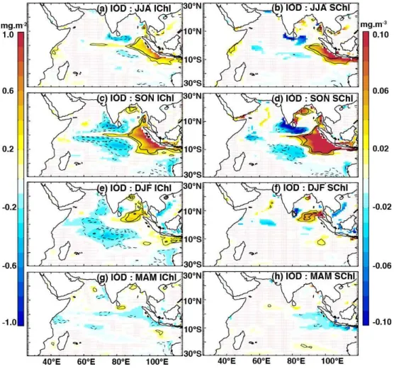
As expected from the widespread relationship seen in Fig. 6c, IOD-related anomalies of IChl show similar (but opposite) patterns to those of D20 (left panels in Fig. 7 and right panels in Fig. 4 respectively). IOD exerts a strik-ing control onIChl, predominantly via its substantial influ-ence on regional thermocline depths. The eastern shoaling of D20 results in enhancedIChl along the Java and Suma-tra coast and in the southeastern BoB, starting in summer (Fig. 7a) and spreading and intensifying in fall (Fig. 7c). While these anomalies largely dissipate in winter along the Java/Sumatra coast, they persist in the SBoB (Fig. 7e). Pos-itiveIChl anomalies in the eastern and northern BoB likely follow from the coastal trapped Kelvin wave that shoals the thermocline around the perimeter of the Bay (Fig. 4b, d, f; Rao et al., 2002). A horseshoe-shaped pattern of nega-tive chlorophyll anomalies develops in the central and west-ern basin in fall, with strongest expression either side of the Equator and greatest persistence in the shallow thermocline
ridge region (Fig. 7c, e), similar to the patterns of IOD-related D20 anomalies (Fig. 4d).
TheSChl signals show spatial patterns that are in many ways similar to those of IChl (Fig. 7a–d): Strong IOD-related positive anomalies develop along the Java and Suma-tra coast, starting in boreal summer and peaking in fall, be-fore dissipating in winter. The bloom in the southeastern BoB starts in fall and persists throughout the winter season. The southwestern coast and southern tip of India display a strong chlorophyll decrease in summer and fall. A notable differ-ence between theSChl andIChl anomalies is that the nega-tive western surface anomalies are less extensive and disap-pear for the most part in winter (Fig. 7f), in contrast to those ofIChl, which remain prominent and propagate westwards during this season (Fig. 7e). This difference is related to the lack of relationship between D20 andSChl (Fig. 6d) as op-posed toIChl (Fig. 6c) in this region. The depressed D20 and subsurface chlorophyll anomalies do not seem to reach surface chlorophyll in these areas in boreal winter.
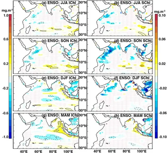
As with D20, the biological response to ENSO is generally weaker and occurs later (Fig. 8) compared to that of the IOD (Fig. 7). PositiveIChl anomalies develop along the eastern boundary in boreal winter and spring (Fig. 8e, g). Concur-rently, lower-than-normalIChl concentrations develop in the wSCTR region between∼8 and 15◦S, and also to a lesser
Fig. 7.The impacts of IOD onIChl (left panels) andSChl (right panels), as indicated by partial regression coefficients of their anomalies regressed onto the IOD index, having removed the influence of ENSO (Eqs. 1–3). Regressions were computed for the period 1961–2001 and their coefficients were drawn only when beyond a 90 % significance level. Thin and thick contours indicate correlation coefficients of 0.4 and 0.6 respectively, while solid (dashed) lines represent positive (negative) correlations.
associated with northeasterly wind anomalies in the western Arabian Sea in boreal fall (Fig. 5d). The Oman and Somalia upwelling systems are likely sensitive to changes in surface winds and these ENSO-related northeasterly anomalies act to reduce upwelling, causing deeper-than-normal thermoclines and warmer-than-normal SSTs (Fig. 5c, d), as well as the chlorophyll impacts noted above.
4.3 Anomalies in key regions
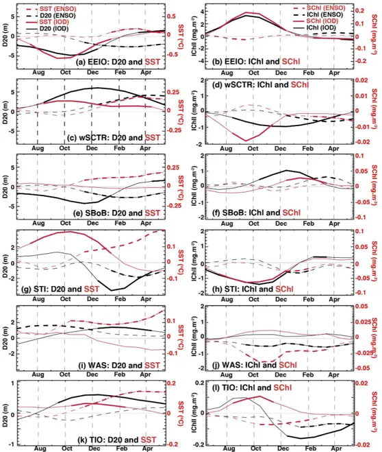
Contrasting Figs. 4 and 5, and 7 and 8, it is clear that the re-sponses to ENSO and IOD forcing differ in space and time. These contrasting impacts, and their seasonality, were more closely examined within specific regions (Fig. 9). There is considerable variability amongst the relative strength and/or state of both climate modes across different years. Plots of the average IChl anomalies versus climate indices during all years (Fig. 10) illustrate this variability and helps vi-sualise the correlative strength between climate mode and
chlorophyll anomalies across different regions. Unexpect-edly, Fig. 10 also revealed an apparent asymmetry in the consequences of the climate modes on chlorophyll concen-trations in some areas.
In the EEIO region, the IOD causes a shoaling of the ther-mocline, and soon thereafter cool SSTs from June/July to December/January (Fig. 9a). The shallow thermocline pro-motes entrainment of nutrients and results in anomalously high surface and integrated chlorophyll concentrations from
∼June/July to December (Fig. 9b). Murtugudde et al. (1999)
J. C. Currie et al.: IOD and ENSO impacts on Indian Ocean chlorophyll 6689
Fig. 8.The impacts of ENSO onIChl (left panels) andSChl (right panels), as indicated by partial regression coefficients of their anomalies regressed onto the ENSO index, having removed the influence of IOD (Eqs. 4–6). Regressions were computed for the period 1961–2001 and their coefficients were drawn only when beyond a 90 % significance level. Thin and thick contours indicate correlation coefficients of 0.4 and 0.6 respectively, while solid (dashed) lines represent positive (negative) correlations.
events. This, together with the statistics in Tables 1 and 2 and the patterns of partial regression coefficients in Figs. 7, 8 and 9 support our conclusion that anomalous phytoplank-ton blooms in the EEIO region are predominantly due to IOD forcing. Figure 10a also suggests that positiveIChl anoma-lies in the EEIO region generally tend to be of greater mag-nitude than negative ones.
In the wSCTR region, deeper thermoclines coincide with warmer surface temperatures in response to ENSO and IOD (Fig. 9c), consistent with results of previous studies (Mey-ers et al., 2007; Rao and Behera, 2005; Xie et al., 2002). The IOD produces slightly earlier thermocline anomalies than ENSO and the ENSO-related surface warming initi-ates and peaks later than that of IOD. ENSO-related chloro-phyll anomalies (both at the surface and over the euphotic layer) seem relatively weak and start to be significant only in boreal winter in this region (Fig. 9d). The clearest bio-geochemical signature is seen in response to IOD, with de-pletedSChl during the IOD peak (∼August to November)
and negative IChl coinciding with the deeper-than-normal D20 signal (∼August to April). Although both IOD and
ENSO are related to significant negative anomalies during DJF (Table 2), the percentage of chlorophyll variability ex-plained by the IOD is far greater than that of ENSO (Table 3). There is no clear asymmetry between positive and negative chlorophyll anomalies in the wSCTR region (Fig. 10b). The largest (negative) anomalies are associated with pure IOD or co-occurring ENSO and IOD events.
Fig. 9.Seasonal evolution of the IOD (solid) and ENSO (dashed) impacts on D20 (black) and SST (red) anomalies in the left column, and IChl (black) andSChl (red) anomalies in the right column, as indicated by partial regression coefficients of these anomalies regressed onto the respective climate index, having removed the influence of the second/remaining climate index (Eqs. 1–3 for solid lines; Eqs. 4–6 for dashed lines). The geographical regions are indicated on Figs. 3 and 6 and described in Sect. 2.3. Bold line segments indicate when partial regression coefficients are beyond the 90 % significance level.
effects. The prominent shoaling of the thermocline in the central SBoB, a result of an upwelling Rossby wave fol-lowing a positive IOD event (Fig. 4f; Wiggert et al., 2009), results in an increase inIChl from∼October to February.
An increase inSChl in response to the shallower nutricline (shoaling thermocline) occurs only during winter (Fig. 9f), likely because winter cooling and stronger winds allow wind-mixing of the surface layers that are otherwise highly strati-fied during the remainder of the year (Prasanna Kumar et al., 2010). PositiveIChl anomalies are seen in response to ENSO
J. C. Currie et al.: IOD and ENSO impacts on Indian Ocean chlorophyll 6691
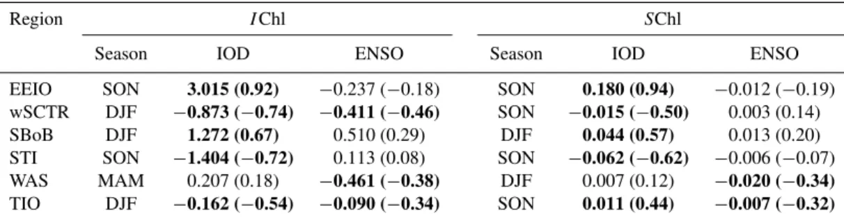
Table 2.Partial regression coefficients (and partial correlation coefficients in brackets) ofIChl (mg m−2)andSChl (mg m−3)anomalies versus the relevant climate index (DMI and Niño3.4). The season selected is that in which the multiple regression including DMI + Niño3.4 explained the greatest proportion ofIChl orSChl variance (which is quoted in Table 3). Bold figures denote significant regression or correlation coefficients (p <0.05).
Region IChl SChl
Season IOD ENSO Season IOD ENSO
EEIO SON 3.015 (0.92) −0.237 (−0.18) SON 0.180 (0.94) −0.012 (−0.19)
wSCTR DJF −0.873 (−0.74) −0.411 (−0.46) SON −0.015 (−0.50) 0.003 (0.14) SBoB DJF 1.272 (0.67) 0.510 (0.29) DJF 0.044 (0.57) 0.013 (0.20) STI SON −1.404 (−0.72) 0.113 (0.08) SON −0.062 (−0.62) −0.006 (−0.07)
WAS MAM 0.207 (0.18) −0.461 (−0.38) DJF 0.007 (0.12) −0.020 (−0.34) TIO DJF −0.162 (−0.54) −0.090 (−0.34) SON 0.011 (0.44) −0.007 (−0.32)
Table 3.Percentage of interannual chlorophyll variance explained by regressions including DMI + Niño3.4 as explanatory variables (first column) and for the partial regression of each climate mode in isolation (2nd and 3rd columns; proportion from Eq. 7 multiplied by 100). The season selected was that in which the multiple regression (first column) explained the greatest proportion ofIChl orSChl variance. Bold figures indicate when partial regressions resulted in a significant coefficient (p <0.05).
IChl SChl
Region Season IOD + IOD ENSO Season IOD + IOD ENSO
ENSO ENSO
EEIO SON 89 62 0 SON 92 64 0
wSCTR DJF 77 27 6 SON 28 24 2
SBoB DJF 68 26 4 DJF 52 23 2
STI SON 60 42 0 SON 53 30 0
WAS MAM 15 3 15 DJF 12 4 11
TIO DJF 56 18 6 SON 20 20 9
In the STI region, a significant shoaling of D20 develops between∼December and April in response to IOD, preceded
by warmer-than-normal SSTs between∼July and January
(Fig. 9g). ENSO events also show warming of surface wa-ters, starting ∼November and growing in magnitude until
May. During much of the same time (∼January to May),
these warm SST anomalies are accompanied by a shoaling thermocline. The main biogeochemical signal is a decrease of both surface and integrated chlorophyll during IOD events (∼June/July to December), while ENSO causes a brief
pe-riod of negative anomalies during winter. During the SON peak expression of climate-mode-related anomalies, the IOD signal completely dominates ENSO in terms of explanatory power of the chlorophyll variability (Table 3). The lack of obvious coupling between thermocline depths and surface temperature or chlorophyll in this region is likely due to in-tense horizontal circulation between the Bay of Bengal and the Arabian Sea (e.g. Vinayachandran et al., 1999), as well as the added complexity of seasonal barrier layers in these regions (Sprintall and Tomczak, 1992). One needs to bear in mind also that mesoscale eddies have been invoked as be-ing important for ecosystem variability in the BoB (Prasanna Kumar et al., 2007), but were not resolved here.
In contrast to all other examined regions, where IOD ex-plains a greater proportion of chlorophyll variability, bio-logical activity in the western Arabian Sea is influenced predominantly by ENSO (Tables 1, 2), causing depressed SChl andIChl anomalies from∼September to the following
Fig. 10.Scatterplots showing the magnitude ofIChl anomalies against climate mode indices across all years (1961–2001).IChl anomalies are averaged over the regions of interest and over the same seasons as selected in Tables 1 and 2, namely:(a)EEIO in SON,(b)wSCTR in DJF,(c)SBoB in DJF,(d)STI in SON,(e)WAS in MAM and(f)TIO in DJF. Climate mode events as identified by Meyers et al. (2007) are indicated by colour: pure IOD events are blue, pure ENSO events red, co-occurring events green and non-event years black. Significant correlation coefficients (p <0.05) betweenIChl and climate indices are provided on the plot or indicated as NS (not significant;p≥0.05). Solid black lines represent the slopes of significant regressions (p <0.05), fit separately to index values>0 and<0. Dashed red lines illustrate loess smooth curves fit by least squares (allowing a non-linear best fit).
monsoon-related forcing may instead play significant roles in affecting interannual anomalies in this region. The IOD seems to have relatively little impact in this region, causing a deeper-than-normal thermocline between∼December and
April, but neither SST nor chlorophyll anomalies. Figure 9j and Tables 1 and 2 point to ENSO but not IOD controlling chlorophyll anomalies in the WAS region.
The integrated influences of IOD and ENSO over the en-tire tropical Indian Ocean basin (TIO) are shown in Fig. 9k and l. At this scale, the IOD has a significant positive ef-fect on D20 from∼September to May, while ENSO seems
J. C. Currie et al.: IOD and ENSO impacts on Indian Ocean chlorophyll 6693
(∼November to May) than for IOD (∼October to
Febru-ary; Schott et al., 2009; Xie et al., 2009). Despite the deeper-than-normal D20 associated with IOD,SChl anomalies show a brief positive period during the IOD peak (∼August to
November), which suggests that the chlorophyll bloom in the eastern pole dominates the basin-wide response during those months. On the other hand, basin-wideIChl becomes signif-icantly less-than-normal in winter and spring in response to IOD (Fig. 9l), driven largely by the horseshoe-shaped neg-ative anomalies in the western basin and thermocline ridge region (Fig. 7e). ENSO-related chlorophyll signals are neg-ative for both surface (∼October to February) and
depth-integrated values (∼January to May), suggestive of an
over-all negative effect on basin-scale chlorophyll concentration. The positive influence of IOD and negative effect of ENSO onSChl likely counter-act one another during years when these events co-occur, such as in 1997 and 2006. Their com-bined effect, however, explains only about 20 % of interan-nualSChl variability (Table 3), which may be additionally affected by further climate or ecosystem dynamics.
5 Summary and discussion
The remotely-sensed chlorophyll record is too short to con-fidently differentiate the relative contributions of IOD and ENSO to interannual variability. A novel contribution of our study is to effectively separate ENSO and IOD impacts within the Indian Ocean and to investigate these in six re-gions, using a 41 yr hindcast from a coupled biophysical general circulation model. Although focus was on the re-sponse of chlorophyll, changes in thermocline depth, surface temperature and surface winds were also assessed in order to gain a better understanding of physical processes driving the biological patterns. In comparison with SeaWiFS data, the modelled SChl showed good qualitative agreement of open-ocean seasonal variability and interannual anomalies during the 1997/1998 El Niño/positive IOD event. This, de-spite lacking some of the spatial contrasts or complexity seen in SeaWiFS (especially in coastal regions), which are likely structured by meso- and smaller-scale processes not resolved by the simulation. As a result, interpretations were intention-ally limited to broad regional patterns.
Although previous studies have not isolated IOD and ENSO signals in chlorophyll anomalies, the patterns de-scribed from co-occurring IOD/ENSO events (Murtugudde et al., 1999; Sarma, 2006; Vinayachandran and Mathew, 2003; Wiggert et al., 2009) are consistent with results pre-sented here. Wiggert et al. (2009) use SeaWiFS chlorophyll records to assess the Indian Ocean response to the two pos-itive IOD/El Niño events of 1997 and 2006, and interpret these in light of physical forcing and their resultant im-pacts on primary productivity. In agreement with our results, they find surface chlorophyll and net primary production in-creases in the eastern tropical Indian Ocean in boreal fall and
in the southeastern Bay of Bengal in winter, as well as neg-ative primary production anomalies in the southwestern In-dian Ocean in fall and winter. Wiggert et al. (2009) note a negative chlorophyll anomaly around the southern tip of In-dia between October and December in both their events. The substantial IOD-forced decrease inIChl (and by deduction primary productivity) in this region has not been established elsewhere to the best of our knowledge.
The IOD produces anomalous dynamic (thermocline depth and Rossby–Kelvin wave) and thermodynamic (mixed layer, SST, and heat flux) variability, with phytoplankton communities responding to the sum total of these dynamical-thermodynamical influences on the upper ocean. Across most of the Indian Ocean,IChl changes are strongly related to anomalies of D20 (Fig. 6c), explained by the importance for phytoplankton productivity of the vertical proximity of high-nutrient subsurface waters to the sunlit euphotic layer (Lewis et al., 1986; Messié and Chavez, 2012; Wilson and Adamec, 2002). Messié and Chavez (2012) recently high-lighted the dominant role of nutricline depths in controlling changes in chlorophyll and productivity at the global scale. As ENSO and IOD are not orthogonal, their analyses would not effectively separate the signatures of these two modes, and their ENSO-correlated EOFs of chlorophyll and produc-tivity likely contain a proportion of IOD-related expression in the Indian Ocean.
There are, of course, regions in the Indian Ocean where neither IOD nor ENSO seem to control chlorophyll anoma-lies. Other drivers not investigated here, such as the Indian monsoon, intra-annual climate perturbations and ecosys-tem dynamics might affect interannual chlorophyll anoma-lies in these regions. The ecosystem could influence chloro-phyll concentration via top-down grazing control, as well as bottom-up nutrient regeneration and fertilisation of sur-face waters by zooplankton and higher trophic levels. A dominance of regenerated production in stratified, nutrient-starved, low-chlorophyll areas is an explanation suggested for the apparent asymmetry in chlorophyll anomalies seen between positive and negative climate events in some regions (Fig. 10). Such an explanation, if correct, would be an ex-ample of ecosystem dynamics mitigating the magnitude of climate-induced negative chlorophyll anomalies.
modes. Our investigation suggests that the interannual vari-ability in this region, including that of chlorophyll, is more strongly related to ENSO forcing than to IOD. These findings are supported by Kao and Yu (2009), who show evidence that El Niño events peaking in the eastern Pacific are related to northeasterly wind anomalies and warmer SST in the west-ern Arabian Sea during June–September. Furthermore, Sy-roka and Toumi (2004) and Xavier et al. (2007) have shown evidence of a shortened summer monsoon linked to El Niño, which would imply a shorter period of active upwelling and likely less productivity in those years.
Due to opposing regional signals, the basin-scale Indian Ocean chlorophyll response to co-occurring events seems to be weak (Fig. 9), as pointed out by Wiggert et al. (2009). Extensive regional re-organisation does take place however, with significant integrated chlorophyll anomalies occurring over periods of several months in certain regions. As phy-toplankton constitute the basal trophic level in pelagic envi-ronments, and by their ecology dictate the pathway of en-ergy flow through the ecosystem (Falkowski et al., 1998), such climate-mode anomalies likely have great repercus-sions for pelagic ecosystems. The disruption of Indian Ocean ecosystems and resources has been attributed to ENSO/IOD events (e.g. Marsac and Le Blanc, 1999; Ménard et al., 2007; Spencer et al., 2000; Vialard et al., 2009), although the nec-essary biological data sets to detect such disruptions at higher trophic levels are often lacking. Through the coordinated ef-fort of international research programs such as SIBER (Hood et al., 2010), by increasing the availability of higher resolu-tion and longer-term data sets of physical, biogeochemical and biological variability, and with the use of rapidly pro-gressing coupled ecosystem models to fill in the gaps, we have increasingly exciting and fruitful avenues available to understand and develop predictability of climate mode im-pacts on the physical and biological Indian Ocean.
Supplementary material related to this article is available online at http://www.biogeosciences.net/10/ 6677/2013/bg-10-6677-2013-supplement.pdf.
Acknowledgements. M. Lengaigne, J. Vialard, D. Kaplan, O.
Aumont and O. Maury are funded by Institut de Recherche pour le Développement (IRD). M. Lengaigne, O. Aumont and O. Maury acknowledge the support of the French ANR, under the grant CEP MACROES (MACRoscope for Oceanic Earth System ANR-09-CEP-003). M. Lengaigne and J. Vialard did part of this work as visiting scientists at the National Institute of Oceanography in Goa, India. IRD funding supported J. Currie throughout his masters degree, from which work this paper was borne, and supported a visit to NIO for him to work on this study with M. Lengaigne and J. Vialard. Thanks are due to Raghu Murtugudde and Marina Lévy for their incisive comments on the manuscript. Two anonymous reviewers are acknowledged for their detailed treatment of the paper, which improved the final product.
Edited by: R. Hood
References
Abram, N. J., Gagan, M. K., McCulloch, M. T., Chappell, J., and Hantoro, W. S.: Coral reef death during the 1997 Indian Ocean Dipole linked to Indonesian wildfires, Science, 301, 952–955, doi:10.1126/science.1083841, 2003.
Abram, N. J., Gagan, M. G., McCulloch, M. T., Chappell, J., and Hantoro, W. S.: Response to comment on “Coral reef death dur-ing the 1997 Indian Ocean Dipole linked to Indonesian wild-fires”, Science, 303, 1297–1297, doi:10.1126/science.1094047, 2004.
Annamalai, H., Murtugudde, R., Potemra, J., Xie, S. P., Liu, P., and Wang, B.: Coupled dynamics over the Indian Ocean: spring ini-tiation of the Zonal Mode, Deep-Sea Res. Pt. II, 50, 2305–2330, doi:10.1016/S0967-0645(03)00058-4, 2003.
Aumont, O. and Bopp, L.: Globalizing results from ocean in situ iron fertilization studies, Global Biogeochem. Cy., 20, GB2017, doi:10.1029/2005GB002591, 2006.
Aumont, O., Bopp, L., and Schulz, M.: What does temporal vari-ability in aeolian dust deposition contribute to sea-surface iron and chlorophyll distributions?, Geophys. Res. Lett., 35, L07607, doi:10.1029/2007GL031131, 2008.
Ballabrera-Poy, J., Murtugudde, R. G., Christian, J. R., and Busalacchi, A. J.: Signal-to-noise ratios of observed monthly tropical ocean color, Geophys. Res. Lett., 30, 1645, doi:10.1029/2003GL016995, 2003.
Baquero-Bernal, A., Latif, M., and Legutke, S.: On dipole-like variability of sea surface temperature in the tropical In-dian Ocean, J. Climate, 15, 1358–1368, doi:10.1175/1520-0442(2002)015<1358:ODVOSS>2.0.CO;2, 2002.
Behrenfeld, M. J., Westberry, T. K., Boss, E. S., O’Malley, R. T., Siegel, D. A., Wiggert, J. D., Franz, B. A., McClain, C. R., Feld-man, G. C., Doney, S. C., Moore, J. K., Dall’Olmo, G., Milli-gan, A. J., Lima, I., and Mahowald, N.: Satellite-detected fluo-rescence reveals global physiology of ocean phytoplankton, Bio-geosciences, 6, 779–794, doi:10.5194/bg-6-779-2009, 2009. Bjerknes, J.: Atmospheric teleconnections from the equatorial
Pacific, Mon. Weather Rev., 97, 163–172, doi:10.1175/1520-0493(1969)097<0163:ATFTEP>2.3.CO;2, 1969.
Blanke, B. and Delecluse, P.: Variability of the tropical Atlantic Ocean simulated by a general circulation model with two dif-ferent mixed-Layer physics, J. Phys. Oceanogr., 23, 1363–1388, doi:10.1175/1520-0485(1993)023<1363:VOTTAO>2.0.CO;2, 1993.
Boyer, T., Levitus, S., Garcia, H., Locarnini, R. A., Stephens, C., and Antonov, J.: Objective analyses of annual, seasonal, and monthly temperature and salinity for the World Ocean on a 0.25◦
grid, Int. J. Climatol., 25, 931–945, doi:10.1002/joc.1173, 2005. Claustre, H., Morel, A., Hooker, S. B., Babin, M., Antoine, D., Oubelkheir, K., Bricaud, A., Leblanc, K., Quéguiner, B., and Maritorena, S.: Is desert dust making olig-otrophic waters greener?, Geophys. Res. Lett., 29, 107–1, doi:10.1029/2001GL014056, 2002.
Cleveland, R. B., Cleveland, W. S., McRae, J. E., and Terpenning, I.: STL: A seasonal-trend decomposition procedure based on loess, J. Official Statist., 6, 3–73, 1990.
J. C. Currie et al.: IOD and ENSO impacts on Indian Ocean chlorophyll 6695
Dandonneau, Y., Vega, A., Loisel, H., Du Penhoat, Y., and Menkes, C.: Oceanic Rossby Waves acting as a “hay rake” for ecosystem floating by-products, Science, 302, 1548–1551, doi:10.1126/science.1090729, 2003.
Djavidnia, S., Mélin, F., and Hoepffner, N.: Comparison of global ocean colour data records, Ocean Sci., 6, 61–76, doi:10.5194/os-6-61-2010, 2010.
Du, Y., Xie, S.-P., Huang, G., and Hu, K.: Role of air– sea interaction in the long persistence of El Niño–induced north Indian Ocean warming, J. Climate, 22, 2023–2038, doi:10.1175/2008JCLI2590.1, 2009.
Falkowski, P. G., Barber, R. T., and Smetacek, V.: Biogeochemical controls and feedbacks on ocean primary production, Science, 281, 200–206, doi:10.1126/science.281.5374.200, 1998. Feng, M. and Meyers, G.: Interannual variability in the tropical
Indian Ocean: a two-year time-scale of Indian Ocean Dipole, Deep-Sea Res. Pt. II, 50, 2263–2284, doi:10.1016/S0967-0645(03)00056-0, 2003.
Geider, R. J., MacIntyre, H. L., and Kana, T. M.: A dynamic reg-ulatory model of phytoplanktonic acclimation to light, nutrients, and temperature, Limnol. Oceanogr., 43, 679–694, 1998. Goosse, H.: Modelling the large-scale behaviour of the coupled
ocean–sea-ice system, Ph.D. thesis, Université catholique de Louvain, Belgium, 1997.
Gordon, H. R. and McCluney, W. R.: Estimation of the depth of sunlight penetration in the sea for remote sensing, Appl. Opt., 14, 413–416, 1975.
Hastenrath, S.: Dipoles, temperature gradients, and tropical climate anomalies, B. Am. Meteorol. Soc., 83, 735–738, doi:10.1175/1520-0477(2002)083<0735:WLACNM>2.3.CO;2, 2002.
Hermes, J. C. and Reason, C. J. C.: Annual cycle of the south Indian Ocean (Seychelles-Chagos) thermocline ridge in a re-gional ocean model, J. Geophys. Res.-Oceans, 113, C04035, doi:10.1029/2007JC004363, 2008.
Hood, R. R., Wiggert, J. D., and Naqvi, S. W. A.: A New Basin-wide, International Program in the Indian Ocean, Ocean Carbon and Biogeochemistry News, 3, 5–8, 2010.
Horii, T., Hase, H., Ueki, I., and Masumoto, Y.: Oceanic precon-dition and evolution of the 2006 Indian Ocean dipole, Geophys. Res. Lett., 35, L03607, doi:10.1029/2007GL032464, 2008. Howden, S. D. and Murtugudde, R.: Effects of river inputs into
the Bay of Bengal, J. Geophys. Res.-Oceans, 106, 19825–19843, doi:10.1029/2000JC000656, 2001.
Iskandar, I., Rao, S., and Tozuka, T.: Chlorophyll-a bloom along the southern coasts of Java and Sumatra during 2006, Int. J. Remote. Sens., 30, 663–671, 2009.
Izumo, T., Vialard, J., Lengaigne, M., de Boyer Montégut, C., Be-hera, S. K., Luo, J.-J., Cravatte, S., Masson, S., and Yamagata, T.: Influence of the state of the Indian Ocean Dipole on the following year’s El Niño, Nat. Geosci., 3, 168–172, doi:10.1038/ngeo760, 2010.
Jackett, D. R. and Mcdougall, T. J.: Minimal adjustment of hydrographic profiles to achieve static stability, J. At-mos. Ocean. Technol., 12, 381–389, doi:10.1175/1520-0426(1995)012<0381:MAOHPT>2.0.CO;2, 1995.
Kao, H.-Y. and Yu, J.-Y.: Contrasting eastern-Pacific and central-Pacific types of ENSO, J. Climate, 22, 615–632, doi:10.1175/2008JCLI2309.1, 2009.
Keerthi, M., Lengaigne, M., Vialard, J., de Boyer Montégut, C., and Muraleedharan, P.: Interannual variability of the Tropi-cal Indian Ocean mixed layer depth, Clim. Dynam., 38, 1–17, doi:10.1007/s00382-012-1295-2, 2012.
Klein, S. A., Soden, B. J., and Lau, N. C.: Remote sea surface temperature variations during ENSO: Evidence for a tropical at-mospheric bridge, J. Climate, 12, 917–932, doi:10.1175/1520-0442(1999)012<0917:RSSTVD>2.0.CO;2, 1999.
Koné, V., Aumont, O., Levy, C., and Resplandy, L.: Physical and biogeochemical controls of the phytoplankton seasonal cycle in the Indian Ocean: A modeling study, in: Indian Ocean Biogeo-chemical Processes and Ecological Variability, vol. 185, edited by: J. D. Wiggert, R. R. Hood, S. Wajih, A. Naqvi, K. H. Brink, and S. L. Smith, p. 350, 2009.
Lengaigne, M. and Vecchi, G.: Contrasting the termination of mod-erate and extreme El Niño events in coupled general circulation models, Clim. Dynam., 35, 299–313, doi:10.1007/s00382-009-0562-3, 2010.
Lengaigne, M., Boulanger, J.-P., Menkes, C., Masson, S., Madec, G., and Delecluse, P.: Ocean response to the March 1997 Westerly Wind Event, J. Geophys. Res.-Oceans, 107, 8015, doi:10.1029/2001JC000841, 2002.
Lengaigne, M., Madec, G., Menkes, C., and Alory, G.: Impact of isopycnal mixing on the tropical ocean circulation, J. Geophys. Res.-Oceans, 108, 3345, doi:10.1029/2002JC001704, 2003. Lengaigne, M., Boulanger, J.-P., Menkes, C., and Spencer, H.:
Influ-ence of the seasonal cycle on the termination of El Niño events in a coupled general circulation model, J. Climate, 19, 1850–1868, doi:10.1175/JCLI3706.1, 2006.
Lengaigne, M., Menkes, C., Aumont, O., Gorgues, T., Bopp, L., André, J.-M., and Madec, G.: Influence of the oceanic biology on the tropical Pacific climate in a coupled general circulation model, Clim. Dynam., 28, 503–516, doi:10.1007/s00382-006-0200-2, 2007.
Lengaigne, M., Hausmann, U., Madec, G., Menkes, C., Vialard, J., and Molines, J.: Mechanisms controlling warm water vol-ume interannual variations in the equatorial Pacific: diabatic versus adiabatic processes, Clim. Dynam., 38, 1031–1046, doi:10.1007/s00382-011-1051-z, 2012.
Lewis, M. R., Hebert, D., Harrison, W., Platt, T., and Oakey, N. S.: Vertical nitrate fluxes in the oligotrophic ocean, Science, 234, 870–873, 1986.
Madec, G., Delecluse, P., Imbard, M., and Lévy, C.: OPA 8.1 Ocean general circulation model reference manual, Note du Pôle de modélisation, IPSL, Paris, 1998.
Maritorena, S., D’ Andon, O. H. F., Mangin, A., and Siegel, D. A.: Merged satellite ocean color data products using a bio-optical model: Characteristics, benefits and issues, Remote Sens. Envi-ron., 114, 1791–1804, doi:10.1016/j.rse.2010.04.002, 2010. Marsac, F. and Le Blanc, J. L.: Oceanographic changes during the
1997–1998 El Niño in the Indian Ocean and their impact on the purse seine fishery, IOTC Proceedings, 2, 147–157, 1999. Maury, O.: An overview of APECOSM, a spatialized mass balanced