Lat. Am. j. solids struct. vol.11 número5

(1)

Abs tract

The analytical solutions for the natural frequencies and mode

shapes of the rectangular plate on foundation with four edges free

is presented by using the finite cosine integral transform method.

In the analysis procedure, the classical Kirchhoff rectangular plate is considered and the foundation is modelled as the Winkler elastic

foundation. Because only are the basic dynamic elasticity equ a-tions of the thin plate on elastic foundation adopted, it is not need prior to select the deformation function arbitrarily. Therefore, the solution developed by present paper is reasonable and theoretical. In order to illuminate the correction of formulations, the numer i-cal results are also presented to comparing with that of the other references.

Key words

Elastic foundation, Rectangular plate with four edges free, natural frequencies Vibration mode shapes, Finite cosine integral tran

s-form

Vibration of Plate on Foundation with Four Edges

Free by Finite Cosine Integral Transform Method

1 IN T R O D U C T IO N

The vibrations of rectangular thin plates with various boundary conditions are of much im-portance in all the fields of civil, mechanical, and aerospace engineering. To conduct an accurate free vibration analysis of rectangular plates is necessary for controlling the resonance thus ensur-ing the safety of plates. Actually, the vibrations of rectangular thin plates have been extensively investigated for many years. The related publications can be counted in thousands, like in Leissa (1993). A literature survey reveals that most previous investigations have dealt with a scheme or technique that is only suitable for a particular type of boundary condition. Due to the mathemat-ical complexity of the situation, it is well known that the analytmathemat-ical solutions are generally avail-able only for plates that are simply supported along at least one pair of opposite edges. Leissa gave a survey of research on rectangular plate problems up to 1970, like in Warburton (1954) and Leissa (1973). The further overview up to the beginning of this century is presented in Warburton (1979) and Warburton & Edney (1984). One of the most commonly used methods in free vibra-tion analysis of plates is the Rayleigh–Ritz energy technique, where appropriate funcvibra-tions

associ-Y an g Z ho ng*, X u e- f en g Z ha o, H en g L i u

Department of Civil Engineering Dalian Uni-versity of Technology P.R.China

Received in 23 Apr 2013 In revised form 20 Jun 2013

(2)

Latin American Journal of Solids and Structures 11 (2014) 854-863

ated with various boundary conditions are chosen to describe the lateral deflection of the de-formed plates. The chosen functions normally do not satisfy both the governing differential equa-tions and boundary condiequa-tions. Gorman used the superposition technique to solve approximately free vibration problems of plates for various geometries and boundary conditions, like in Gorman (1980) and Gorman (1982). A set of static beam functions was used to determine the natural frequencies of elastically restrained plates, like in Bapat et al (1988) and Zhou (1996). Hurlebaus et al. (2001) have extended the Fourier series solution to the problems with more complicated boundary conditions than the simply supported one. The other numerical approaches such as the finite element method as in Yang (1972) and boundary element method as in Zafrang (1995) were usually adopted by many researchers to analyze the plate on elastic foundation.

Integral transform is one of the effective approaches to obtain the analytical solutions of some partial differential equations used in elasticity, like in Sneddon (1972). This method has often been utilized to analyze some structural engineering problems, like in Sneddon (1981). How-ever, based on the author’s knowledge, there are no reports on using the finite integral transform to analyze the rectangular plate on elastic foundation, like in Zhong et al (2009), Li et al (2009), Li et al (2011) and Li et al (2013).

In this paper, the double finite cosine integral transform method is adopted to acquire the theoretical solutions of eigenfrequncies and vibration modes for the rectangular thin plate on foundation with four edges free. In the analysis the elastic foundation was modeled by the Win-kler elastic foundation. Because it only uses the basic dynamic elasticity equations of the thin plate on elastic foundation and there is no need to select the deformation function arbitrarily, the developed solution is reasonable. In order to proof the correction of formulations, the numerical results are presented to compare with those from other references.

2 V IB R A T IO N O F P LA T E O N FO U N D A T IO N A N D IN T EG R A L T R A N SFO R M

According to the theory the classical Kirchhoff plate, the governing equation of motion for an unloaded plate on the foundation is

∂

4

w

∂

x

4

+

2 ∂

4

w

∂

x

2

∂

y

2

+

∂

4

w

∂

y

4

+

k

D

w

(

x

,

y

,

t

)

+

ρ

h

D

∂

2

w

∂

t

2

=

0

(1)

where

D

₌

Eh

3

_{/ 12(1}

₋

v

2

₎

_{is the flexural rigidity of plate. In which}

_E

_{is Young’s moduli. Also} is Poisson’s ratios.

h

_and

_ρ

_{are the thickness and the density of plate.}

_w

(

x

,

y

,

t

)

is the out-of-plane displacement and k is the reaction coefficient of foundation. Assuming a harmonic vibration, one way write

w

(

x

,

y

,

t

)

₌

W

(

x

,

y

)

Sin

ω

_t

₍₂₎

where

W

(

x

,

y

)

is the shape function describing the modes of the vibration and

ω

_{is the natural}

(3)

∂

4

W

∂

_x

4

+

2 ∂

4

W

∂

_x

2

∂

_y

2

+

∂

4

W

∂

_y

4

+

λ

W

=

0

(3)

where

λ

=

k

−

ρ

h

ω

2

D

In order to solve the partial differential equation (3), the double finite cosine integral trans-form approach[11] is exploited.

If

f

(x,

y)

is a function of the two independent variables

x

_and

_y

_{, defined on the square}

0 _<

x

_<

a

_,

0 _<

_y

_<

_b

_{, the definition of double finite cosine integral transform is presented by the}

equation

f

(

m

,

n

)

=

f

(

x

,

y

)

cos

0

b

∫

0

a

∫

α

_m

xcosβ

_n

ydxdy

(4)

The inversion formula can be derived as

f

(x,

y)

₌

1 ab

f

(0,0)

+

2 ab

f

(m,0)cos

α

m

x

+

2 ab

f

(0,

n)cos

β

n

y

n=1

∞

∑

m=1 ∞

∑

+

4 ab

n=1

f

(

m

,

n

)

cos

α

m

xcos

β

n

y

∞

∑

m=1

∞

∑

(5)

where

α

m

=

mπ

/

a

and

β

n

=

n

π

/

b

.

a

and

b

are the length and the width of the plate

respec-tively.

The double integral transform of the first partial derivative term appeared in Eg.(3) may read-ily be written as

∂

4

W

∂

x

4

cos

0 b

∫

0 a

∫

α

_m

xcos

β

_n

ydxdy

₌

α

m

4

W

₍

m

_,

n

₎

₊

(

−

1)

m

∂

3

W

∂x

3

x=a

−

∂

3

W

∂x

3

x=0

−

α

_m2

(

−

1)

m

∂W

∂x

_x =a

−

∂

W

∂x

_x

=0

⎡

⎣

⎢

⎤

⎦

⎥

⎧

⎨

⎪

⎩⎪

⎫

⎬

⎪

⎭⎪

cosβ

n

y dy

0

b

∫

(6)

(4)

∂

4

W

∂

y

4

cos

0

b

∫

0

a

∫

α

_m

xcosβ

_n

ydxdy

₌

β

_n4

W

(

m

,

n

)

₊

(−1)

n

∂

3

W

∂

y

3

y=b

−

∂

3

W

∂

y

3

y=0

−

β

_n2

₍₋₁₎

n

∂

W

∂

y

_y₌_b

−

∂W

∂

y

_y₌₀

⎡

⎣

⎢

⎤

⎦

⎥

⎧

⎨

⎪

⎩⎪

⎫

⎬

⎪

⎭⎪

cosα

_m

x dx

0

a

∫

(7)

The second term is split into two parts. The first part considers the partial derivative with re-spect to y first

∂

4

W

∂

x

2

∂

y

2

cos

0 b

∫

0 a

∫

α

_m

xcos

β

_n

ydxdy

=

(

−

1)

n

∂

W

∂

y

_y

=b

−

∂

W

∂

y

_y

=0

⎡

⎣

⎢

⎤

⎦

⎥

cos

α

m 0

a

∫

xdx

+

(−1)

m

∂

3

W

∂

x

∂

y

2

x=a

−

∂

3

W

∂

x

∂

y

2

x=0

⎡

⎣

⎢

⎤

⎦

⎥

cos

β

n

y dy

+

α

m 2

_β

n 2

W

(

m

,

n

)

0

b

∫

(8)

while the second part considers the partial derivative with respect to x first

∂

4

W

∂

x

2

∂

y

2

cos

0

b

∫

0 a

∫

α

_m

xcos

β

_n

ydxdy

=

(

−

1)

m

∂

W

∂

x

x=a

−

∂

W

∂

y

x=0

⎡

⎣

⎢

⎤

⎦

⎥

cos

β

_n 0

b

∫

ydy

+

(

−

1)

n

∂

3

W

∂

x

2

∂

y

y=b

−

∂

3

W

∂

x

2

∂

y

y=0

⎡

⎣

⎢

⎤

⎦

⎥

cos

α

m

x dx

0

a

∫

+

α

m

2

_β

n 2

W

(m,

n)

(9)

Substitution of equations (6-9) into equation (3) leads to

[(

α

m 4

+

2 α

m 2

β

n 2

+

β

n 4

)

₊

λ

]

W

₍

m

_,

n

₎

₌

−

(

α

_m2

₊

νβ

_n2

)

(

−

1)

n

∂

y

∂

2

W

∂

x

2

+

∂

2

W

∂

y

2

⎛

⎝⎜

⎞

⎠⎟

_y=b

−

∂

y

∂

2

W

∂

x

2

+

∂

2

W

∂

y

2

⎛

⎝⎜

⎞

⎠⎟

_y=₀

⎧

⎨

⎪

⎩⎪

⎫

⎬

⎪

⎭⎪

cos

α

_m

x dx

0

a

∫

\

+

(α

m

2

+

νβ

n

2

₎

₍₋₁₎

n

∂

W

∂

y

_y=b

−

∂

W

∂

y

_y=₀

⎡

⎣

⎢

⎤

⎦

⎥

cos

α

m

0

a

∫

xdx

−(

β

n 2

+

να

m 2

)

(−1)

m

∂

x

∂

2

W

∂

x

2

+

∂

2

W

∂

y

2

⎛

⎝⎜

⎞

⎠⎟

_x =a

−

∂

x

∂

2

W

∂

x

2

+

∂

2

W

∂

y

2

⎛

⎝⎜

⎞

⎠⎟

_x =0

⎧

⎨

⎪

⎩⎪

⎫

⎬

⎪

⎭⎪

cos

β

_n 0

b

∫

ydy

+

(β

n

2

+

να

m

2

)

(

−

1)

m

∂

W

∂

x

_x =a

−

∂

W

∂

x

_x

=0

⎡

⎣

⎢

⎤

⎦

⎥

cos

β

_n 0

b

∫

ydy

(5)

The boundary conditions of a free plate are[15]

Q

_x

=

−

D

∂

∂x

∂

2

W

∂x

2

+

∂

2

W

∂y

2

⎛

⎝⎜

⎞

⎠⎟

=

0

at

x

=

0

and

x

=

a

(11)

M

_x

₌

−

_D

₍

∂

2

W

∂

x

2

+

v

∂

2

W

∂

y

2

)

=

0

at

x

₌

0

_and

x

₌

a

₍₁₂₎

M

_xy

₌

−

D(1

−

v)

∂

2

W

∂

_x

∂

_y

=

0

at

x

₌

0

_and

x

₌

a

₍₁₃₎

Q

y

=

−

D

∂

y

∂

2

W

∂

x

2

+

∂

2

W

∂

y

2

⎛

⎝⎜

⎞

⎠⎟

=

0

at

y

=

0

and

y

=

b

(14)

M

_y

₌

−

D

(

∂

2

W

∂

_y

2

+

v

∂

2

W

∂

_x

2

)

=

0

at

y

=

0

and

y

=

b

(15)

M

_xy

=

−

_D

(1

−

_v

)

∂

2

W

∂

_x

∂

_y

=

0

at

y

=

0

and

y

=

b

(16)

Of cause, there is another simplified expression of the boundary conditions for a free plate. Substituting the boundary conditions that are described by equation (11) and equation(14) into equation(10), one can obtain

[(

α

m 4

+

2 α

m 2

_β

n 2

+

β

n 4

₎

+

λ

]

W

₍

m

_,

n

₎

₌

+

(

α

_m2

+

νβ

n

2

)

(

−

1)

n

∂

W

∂

y

_y

=b

−

∂

W

∂

y

_y

=0

⎡

⎣

⎢

⎤

⎦

⎥

0

a

∫

cos

α

_m

xdx

+

(

β

_n2

+

να

m

2

)

(

−

1)

m

∂

W

∂

x

_x₌_a

−

∂

W

∂

x

_x₌₀

⎡

⎣

⎢

⎤

⎦

⎥

0

b

∫

cos

β

_n

ydy

(17)

Because the right-hand side of the equation 17 is definite integral, it is the constant. Let

I_m= (−1)n∂W

∂y _y

=b

−∂W ∂y _y

=0

⎡

⎣ ⎢ ⎢

⎤

⎦ ⎥ ⎥

0 a

∫

⋅cosα_mxdx;

J

n

=

(

−

1)

m

∂

W

∂

x

_x

=a

−

∂

W

∂

x

_x

=0

⎡

⎣

⎢

⎤

⎦

⎥

0

b

∫

⋅

cos

β

_n

ydy

(6)

W

₍

m

_,

n

₎

₌

I

m

(

α

m

2

+

νβ

n

2

)

+

J

n

(

β

n

2

+

να

m

2

)

(

α

m

4

+

2 α

m

2

β

n

2

+

β

n

4

)

+

λ

(18)

Substitution of equation (18) into equation (5) gives

W

(

x

,

y

)

₌

(

C

_m₀ m=1

∞

∑

I

_m

+

D

_m₀

J

₀

)

cosα

_m

x

+

(

C

₀_n n=1

∞

∑

I

₀

+

D

₀_n

J

_n

)

cosβ

_n

y

+

2 C

_mn

I

_m

+

D

_mn

J

_n

)

n=1

∞

∑

m=1

∞

∑

cosα

_m

xcosβ

_n

y

(19)

where

C

mn

=

I

m

(

α

m

2

+

νβn

2

)

(

α

m 4

+

2 α

m 2

βn

2

+

βn

4

)

+

λ

；

D

mn

=

J

n

(

β

n

2

+

να

m

2

)

(

α

m

4

+

2 α

m

2

β

n

2

+

β

n

4

)

+

λ

It is clear that the equation 19 can meet the boundary conditions described by equations (11) ,(13) ,(14) and (16). From the remaining boundary conditions presented by equations (12) and (15), one can obtain

α

_m2

(

C

_m0

I

_m

+

D

_m0

J

₀

)

m=1 ∞

∑

+

v

(

β

_n2

C

_0n

I

₀

+

D

_on

J

_n

)

cosβ

_n

y

n=1

∞

∑

+

2 (

α

_m2

+

vβ

_n2

)(

n=1 ∞

∑

m=1 ∞

∑

C

_mn

I

_m

₊

D

_mn

J

_n

)

cosβ

_n

y

₌

0

(20)

(−1)

m

α

_m2

(

C

_m₀

I

_m

+

D

_m₀

J

₀

)

m=1 ∞

∑

+

v

β

_n2

(

C

₀_n

I

₀

+

D

₀_n

J

_n

)

cosβ

_n

y

n=1

∞

∑

+

2 (−1)

m

(

α

_m2

+

vβ

_n2

)(

n=1 ∞

∑

m=1 ∞

∑

C

_mn

I

_m

+

D

_mn

J

_n

)

cosβ

_n

y

=

0

(21)

β

n 2

(

C

0n

I

0

+

D

0n

J

n

)

n₌1

∞

∑

+

v

_α

m 2

(

C

m0

I

m

+

D

m0

J

0

)

cos

α

m

x

m₌1

∞

∑

+

2 (β

n 2

+

v

_α

m 2

)(

n₌1 ∞

∑

m₌1 ∞

∑

C

mn

I

m

+

D

mn

J

n

)

cos

α

m

x

=

0

(22)

(

−

1)

n

βn

2

(

C

0n

I

0

+

D

0n

J

n

)

n₌1

∞

∑

+

v

_α

m 2

(

C

m0

I

m

+

D

m0

J

0

)

cos

α

m

x

m₌1

∞

∑

+

2 (

−

1)

n

(

β

n

2

+

v

_α

m 2

)(

n₌₁ ∞

∑

m₌₁ ∞

∑

C

mn

I

m

+

D

mn

J

n

)

cos

α

m

x

=

0

(7)

Equations 20 and equation 21 make

α

_m2

(

C

_m₀

I

_m

+

D

_m₀

J

₀

)

m=1,3,5

∞

∑

+

2 (

α

_m2

+

v

β

_n2

)(

C

_mn

I

_m

+

D

_mn

J

_n

)

m=1,3,5

∞

∑

⎡

⎣

⎢

⎤

⎦

⎥

n=1

∞

∑

⋅

cos

β

_n

y

=

0

(24)

Similarly, equations (23) and (24) make

β

n 2

(

C

0n

I

0

+

D

0n

J

n

)

n₌1,3,5

∞

∑

+

2 (

β

n

2

+

v

α

m 2

)(

C

mn

I

m

+

D

mn

J

n

)

n₌1,3,5

∞

∑

⎡

⎣

⎢

⎤

⎦

⎥

m₌1 ∞

∑

⋅

cos

α

m

x

=

0

(25)

Each coefficient of the

cos

α

m

x

and

cos

β

n

y

has to be vanish. What follows is a system of homogeneous algebraic equations

α

m

2

(

C

m0

I

m

+

D

m0

J

0

)

m₌1,3,5 ∞

∑

=

0 (α

m

2

+

v

_β

n

2

)(

C

mn

I

m

+

D

mn

J

n

)

m₌1,3,5

∞

∑

=

0 β

n

2

(

C

0n

I

0

+

D

0n

J

n

)

n₌1,3,5

∞

∑

=

0 (β

n

2

+

v

_α

m

2

)(

C

mn

I

m

+

D

mn

J

n

)

n₌1,3,5

∞

∑

=

0

(26)

Eqs. (26) forms the system of four groups of an infinitely large number of linear equations in terms of the unknowns

I

m

,

J

n

,

I

0 and

J

0. Non-trivial solution of those equations requires the coefficient matrix to vanish to any desired degree of accuracy. Non-trivial solution of Eqs. (26) requires the coefficient matrix to vanish. From this determinant the eigenfrequencies of the plate are calculated. The associated vibration modes are given by equation 19 after inserting the eigenfrequencies. The infinite series that occur in the corresponding equations (see Eqs. (19) and (26)) have been evaluated without any truncation using MATLAB[15]; this has been done by spec-ifying the upper limit of the summation index as infinity. The evaluation is exact since corre-sponding closed-form equivalents are automatically substituted in MATLAB.

3 N U M ER IC A L R ESU LT S

(8)

material properties are given as

a

₌

b

₌

4.0

_m,

ν

₌

0.15

_,

E

=

3.0 ×

10

4

MPa,

h

₌

0.2

_m,

k

₌

5.5 _×

10

7_N/m3 _and

_ρ

₌

1750

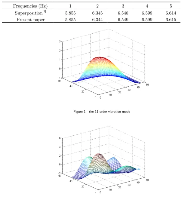
_kg/m3

In order to make the comparison with other method, the eigenfrequencies and the vibration modes are computed by the superposition method[7] and by the present approach. The calculation results are shown in Table 1. It is obvious that the results by two different methods are in excel-lent agreements. This also validates the present approach is correct. Fig. 1 - 4 illuminates the corresponding vibration modes respectively.

Table 1 the nature frequencies of a plate

Frequencies (Hz} 1 2 3 4 5

Superposition[7] 5.855 6.345 6.548 6.598 6.614 Present paper 5.855 6.344 6.549 6.599 6.615

Figure 1 the 11 order vibration mode

(9)

4 C O N C LU SIO N S

(10)

im-Latin American Journal of Solids and Structures 11 (2014) 854-863

portance for many applications such as in the design of building foundations and the rigid pave-ments of highway and airport, the present approach of analysis provides an efficient procedure for accurate results which should be of academic and practical importance.

References

Bapat, A. V., Venkatramani, N., Suryanarayan, S., (1988), Simulation of classical edge conditions by finite elastic restraints in the vibration analysis of plates, Journal of Sound and Vibration 120: 127–140.

Gorman, D.J., (1980), A comprehensive study of the free vibration of rectangular plates resting on symmetri-cally distributed uniform elastic edge supports, Journal of Applied Mechanics 56: 893–899.

Gorman, D.J., (1982), Free Vibration analysis of rectangular plates Elsevier North Holland, Inc.

Hurlebaus, S. L., Gaul, J., Wang, T. S., (2001), An exact series solution for calculating the natural frequencies of orthotropic plates with completely free boundary, Journal of Sound and Vibration 244: 747–759.

Leissa, A.W., (1993), Vibration of Plates, Acoustical Society of America.

Leissa, A.W., (1973), The free vibrations of rectangular plates, Journal of Sound and Vibration 31: 257–293. Li, R., Zhong, Y., Tian, B., Liu, Y.M., (2009), On the finite integral transform method for exact bending solu-tions of fully clamped orthotropic rectangular thin plates. Applied Mathematics Letters 22: 1821-1827.

Li, R., Zhong, Y., Tian, B., (2011), On new symplectic superposition method for exact bending solutions of rectangular cantilever thin plates. Mechanics Research Communications 38: 111-116.

Li, R., Zhong, Y., Li, M.L., (2013), Analytic bending solutions of free rectangular thin plates resting on elastic foundations by a new symplectic superposition method. Proceedings of the Royal Society A 46: 468-474

Sneddon, Ian. H., (1972), The use of integral transforms McGraw-Hill, Inc.

Sneddon, Ian. H., (1981), The application of integral transform in elasticity McGraw-Hill, Inc.

Warburton, G.B., (1954), The vibrations of rectangular plates, Proceeding of the Institute of Mechanical En-gineers, Series A 168: 371–384.

Warburton, G.B., (1979), Response using the Rayleigh–Ritz method, Journal of Earthquake Engineering and Structural Dynamics 7: 327–334.

Warburton, G.B., Edney, S.L., (1984), Vibrations of rectangular plates with elastically restrained edges, Jour-nal of Sound and Vibration 95: 537–552.

Yang, T.Y., (1972), A finite element analysis of plate on two parameters foundation model, Computer and Structure 2: 573-616

Zafrang, A.E., (1995), A new fundamental solution for boundary element analysis of thick plate on Winkle foundation, Int. J. Num. Eng. 38: 887-903

Zhong, Y., Li, R., Liu, Y.M., Tian, B., (2009), On new symplectic approach for exact bending solutions of moderately thick rectangular plates with two opposite edges simply supported. International Journal of Solids and Structures 46: 2506-2513.