ABSTRACT: In this paper, we develop a parametric model method and simulate the deployment mechanism of inlatable antenna structures. Different folded methods are developed for the primary members of inlatable antenna structures, which include inlatable tubes, an inlatable torus, a relector etc. The unstressed coniguration and the folded coniguration of these members are modeled parametrically using the developed folded methods. A simulation software is developed for the deployment mechanism of inlatable structures by the improved spring-mass system. The driving forces in the deployment process, i.e. the gas pressure and the moment of the fold hinges, are analyzed for each member. During the development process, self-contact or collision with the membrane occurs. A rule for identifying self-contact elements is applied, and a penalty function method is developed to solve this challenging problem. Finally, the equation of motion is solved using inite difference method. The developed simulation software is validated by simulating a cylindrical inlatable tube that is folded in half, and the simulation agrees well with the experiment. The deployment mechanism of the antenna model similar to that for the Inlatable Antenna Experiment (IAE) is modeled, analyzed and estimated. The deployed conigurations and the dynamic parameters of each node are obtained. The numerical simulation results show that the simulation software for the deployment mechanism can correctly predict the deployment process of inlatable antenna structures.
KEYWORDS: Inlatable antenna, Improved spring-mass system, Folded methods, Deployment mechanism simulation.
Parametric Model Method and
Deployment Simulation of Inlatable
Antenna Structures
Xu Yan1, Zheng Yao1, Guan Fuling2, Huang He2, Xu Xian2
INTRODUCTION
Large-size aerospace structures are difficult to construct because of the limitations of their weight and launch volume. Compared to conventional electromechanical deployable structures (Xu et al., 2012), the inflatable structures offer many advantages including design flexibility, lightness in weight and compact launch volumes and are suitable for large-size aerospace structures. Since the 1990s, inflatable technologies have been used for antenna structures in NASA’s Jet Propulsion Laboratory etc. Many ideas, concepts and models have been proposed, from the inflatable antenna (Cliff and Ron, 2001; David, 2003) to the inflatable aerodynamic decelerator (Kramer et al., 2013) and the lunar habitat (Capua et al., 2011). One of the key technologies of these structures is that the system can be folded into a compact launch volume and deployed in a smooth and orderly manner. Numerical simulations are needed to investigate the deployment mechanism in greater detail.
Deployment simulations and research studies of inflatable structures to date have primarily focused on inflatable tubes. Simulations have been based on two methods: multi-rigid-body dynamics theory and the non-linear finite element method. In the first simulation method, an inflatable membrane tube is modeled as several rigid struts or beam elements, and the deployment process of the tube can then readily be analyzed using multi-body dynamics theory (Fang et al., 2006). A tube between a two-fold point as inflatable cantilever beams was modeled (Clem and
Smith, 2000), which was then analyzed using multi-rigid-body dynamic theory. The 3-D deployment mechanism of the inflatable structures must be analyzed using the non-linear finite element method (Wang and Johnson, 2002; Lampani and Gaudenzi, 2010) and some commercially available software was applied to this simulation work. PAM-CRASH software was used to simulate the deployment of an inflatable structure (Haug et al., 1991; Katsumata et al., 2014). LS-DYNA software was used to analyze the deployment of a tube and accounted for the reciprocity between the gas low and the lexible tube shell (Salama et al., 2001). The numerical and experimental investigations on the deployment of inflatable tubes with one fold point were conducted (Miyazaki and Uchiki, 2002; Bouzidi et al., 2013). Also the deployment of an inflatable tube was validated by space experiment (Wei et al., 2015). However, only a few research studies have been performed on the deployment mechanism of complicated inflatable structures, which should be investigated further.
For complicated inlatable structures — such as an inlatable antenna, which consists of inlatable tubes, an inlatable torus and a relector —, it is diicult to model the folded coniguration
of the entire structure. In this paper, we report on recent eforts todevelop a parametric model and deployment simulation sotware for inlatable antenna structures. he entire antenna structure is modeled parametrically and analyzed, and the deployment mechanism is simulated using an improved spring-mass system in which the self-contact of the membrane is solved using a penalty function method.
FOLDED METHODS AND
PARAMETRIC MODEL
here are four conigurations in the deployable simulation of inlatable structures: the unstressed coniguration (prior to folding), the initial folded coniguration, the conigurations during deployment and the inal fully deployed coniguration. he purpose of the deployment simulation is to simulate the motion from the initial folded coniguration to the fully deployed coniguration using the known unstressed and the initial folded conigurations. In this section, the unstressed and initial folded conigurations of the primary members, such as the inlatable tubes, the inlatable torus and the relector, are designed and modeled parametrically.
INFLATABLE TUBES
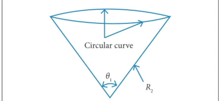
he unstressed coniguration of the inlatable tubes is a cylinder shell. he length of the cylinder shell is L1 and the section radiusis R1. he unstressed coniguration of the section is a circle, and the folded coniguration of the section is shown in Fig. 1, which includes two sections of circular curves. he radius of two circular curves is R2 and the corresponding central angle is θ. he strain of the membrane material during the folding process is neglected, which results in an invariant circumference for the tube section. So, the central angleθ1 in the folded coniguration can be expressed as follows:
Circular curve
R2 θ1
Figure 1. Folded coniguration of the tube’s section.
he coordination of each node in the circular curves can then be calculated. here are typically two folded patterns for inlatable tubes along the length direction: the curve folded pattern and the zigzag folded pattern. he second folded pattern is used for the inlatable antenna structures (Katsumata et al., 2014).
θ1 = (πR1)/R2 (1)
INFLATABLE TORUS
he unstressed coniguration of the inlatable torus is a circular shell surface. his surface has a non-zero Gaussian curvature, which causes an initial stress to appear in the membrane ater the folding process. Similarly to the inlatable tubes, the unstressed coniguration of a section of a torus is a circle, which can be folded in the same way as for the inlatable tubes.
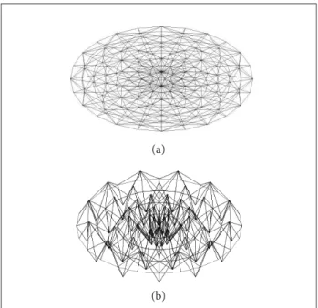
he axes curve of the inlatable torus is also a circle and the radius of the axes curve is denoted by R. he developed folded method is shown in Fig. 2a. A circular curve can be approximated by an equilateral polygon. he number of sides of the equilateral polygon is denoted by n. he length of each side of the polygon is given as follows:
he projected shape in the 0XY plane is also a polygon ater the inlatable torus is folded. θ is the folded angle of each polygon side along vertical direction. he length of each side is given as follows:
he circumradius of the polygon in the folded conigu-ration is:
he projected height of the folded coniguration onto the 0XZ plane is:
hus, the coordination of each fold point is:
where:
φ: the corresponding central angle, and the sign of the Z-coordinate alternates.
he folded methods for the axes curve are used for the torus section to calculate the coordination of each node in the folded coniguration. he folded coniguration of the inlatable torus is shown in Fig. 2b.
INFLATABLE REFLECTOR
he inlatable relector consists of a relectivesurface and a canopy. he relective surface assumes a parabolic shape under the inlation pressure. A parabolic surface is diicult to fold. he
parabolic surface is a surface of revolution; thus, the surface is irst folded along the longitudinal direction and then along the circumferential direction. he fold pattern along the latitudinal direction is similar to that along the axes direction of the inlatable torus. he fold pattern along the latitudinal direction is similar to that of the Z-folded method for inlatable tubes.
he fold pattern of the canopy is similar to that of the relector surface. First, the canopy is placed near the relector surface. he Z-coordination of each point on the canopy is 1 mm smaller than the corresponding point on the reflector surface. The canopy is then folded synchronously with the relector surface. he parametric models for unstressed coniguration and folded coniguration of inlatable relector are shown in Fig. 3.
Figure 2. Parametric model for folded torus. (a) Folded method for axes curve; (b) Folded coniguration. Lxy = (2πR/n)cosθ
Lxy = (2πR/n)sinθ
xi= r cosφi , yi= r sinφi , zi = ±Lxz/2
r = Lxy(R/L)
(b) (a) (3)
(5)
(6) (4)
Z
X
R
θ Lxz r
Y 0
Figure 3. Parametric models of inlatable relector. (a) Unstressed coniguration; (b) Folded coniguration.
(b) (a)
INFLATABLE ANTENNA
cables. he support structure for the inlatable antenna structure consists of three tubes and a torus. here are several tension cables between the relector and the support structure. Each primary member is folded using the developed method and is assembled to form the initial coniguration of the entire structure. he unstressed coniguration and the folded coniguration of the entire antenna structure are shown in Fig. 4.
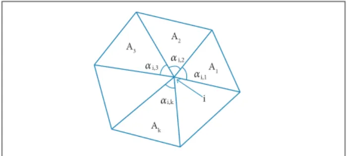
he mass of point i is determined by the area of the membrane elements shown in Fig. 6 and is given as follows:
Figure 4. Parametric models of the entire antenna’s structure. (a) Unstressed coniguration; (b) Folded coniguration.
Figure 5. Spring-mass system. Y
2 3
1
X N1
θ 3
3
2
1 θ
2
θ 1
N 2 N
3
α
α α
where:
ρ: area density of the material; Ak: area of element k around the mass point i; s: number of elements around the mass i; αi: internal angle for each vertex of the element.
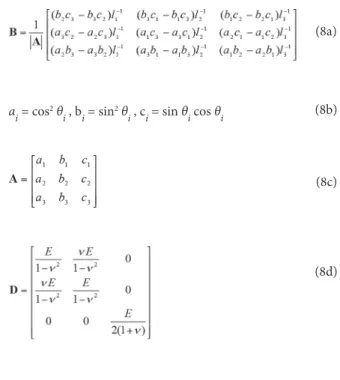
he tension vector of the springs in the element can be obtained from Xu et al. (2007):
where:
δ: extension vector of the three springs; V: volume of the triangular element; D: elastic matrix of the membrane material; B: the relationship matrix between the strains of the element and the length deformations of three springs.
where:
E: elastic modulus; v: Poisson’s ratio; li: initial lengths of the springs; θi : angles that the sides of the element make with the X-axis.
(b) (a)
YZX
Y X
Z
DEPLOYMENT DYNAMICS
SIMULATION METHOD
DESCRIPTION OF SPRING-MASS SYSTEM A spring-mass system is developed to model the membrane material in the deployment simulation. he three vertexes of the triangular membrane element consist of masses, and the three borders consist of springs. he lengths of the springs in their initial state correspond to the original lengths of the springs. During the deployment process, the spring lengths do not equal their original lengths, i.e. internal forces exist in the springs. he three masses move under the combined action of the spring forces and the external forces to reach the inal equilibrium coniguration. he spring-mass system for an element is shown in Fig. 5.
k = 1 s
(7)
(8)
(8a)
(8b)
(8c)
(8d)
ai= cos2θ
i , bi = sin
2θ
DEPLOYMENT DRIVING FORCES
In this section, the deployment driving forces that lead to the motion of the inlatable primary members are formulated. he driving forces in the inlatable antenna structures have two sources: the gas pressure and the moment of the fold hinge.
The internal chamber of the inflatable tubes and the inlatable torus are divided into a inite number of compartments (Katsumata et al., 2014; Xiao et al., 2010). he inlatable relector can be considered to be a compartment. he variations in the gas state of each compartment are functions of the deployment time. the temperature and pressure of the inlation gas are also assumed to be uniform within the control volume of an individual compartment. For each compartment, a set of diferential governing equations based on gas dynamic theory
can be obtained. For three adjacent compartments, i, j and k,
the diferential governing equations for compartment j are given in Eq. 9. For brevity, the formulas are not derived here: further details can be found in Fang et al. (2006).
where:
Ti , mi , Pi , and Vi: temperature, mass, pressure and volume of compartment i; Tj, mj, Pj, and Vj: temperature, mass, pressure and volume of compartment j; Pa: ambient gas pressure;
R = 8.3145 J/molK; k = cp/cv: speciic heat ratio of the gas;
min: mass rate of the gas flowing into compartmentj from compartment i; mout: mass rate of gas lowing out of compartment
j into compartment k.
The state of each compartment is then calculated by integrating this group of diferential equations with respect to the deployment time. he Runge-Kutta method is used to integrate these equations numerically. he inlationpressure of each compartment is then obtained by performing a gas flow analysis and equals the nodal forces on the mass of the spring-mass system. he nodal forces Fa of a triangular element a in the shell of compartment i can be expressed in the following form:
Ak
A3 A2
A1
i
i,3 i,2
i,1
i,k α α α
α
Figure 6. Triangular elements around mass i.
where:
px = nx x Pi , py = ny x Pi , pz = nz x Pi; Pi: pressure of compartmenti;
nx ,ny ,nz : normal vector components of the triangular element plane; A: area of the element.
A non-linear joint model and the Bernoulli-Euler method (Clem and Smith, 2000) were used to obtain the relationship between the restoring moment at a hinge point between two
adjacent compartments and the folded angle θ:
(10)
(11)
.
.
i
i
Fa = (1/3)A{px py pz px py pz px py pz}
M = πpr3[1-exp(-3.12Et/p tan θ/2)]
where:
p: inlation pressure of the tube or torus near this fold joint; r: section radius of the member; E and t : Young’s modulus and the thickness of the material, respectively.
he restoring moment can easily be transformed into the equivalent nodal forces of the mass point in the spring-mass system.
SELF-CONTACT PROBLEM
Membrane collision during the deployment process of the inlatable structures is commonly referred to as the self-contact problem. he self-contact problem is one of the major challenges in a deployment simulation because each thin film moves independently in a 3-D space. One solution for this problem
(9)
Ti
mi
Pi
Vi
Tj
mj
Pj
Vj
.
.
.
.
.
.
.
.
min min
m
.
out.
.
.
.
.
.
.
.
.
.
.
is to apply the polygon intersection method, which identiies membrane collision by determining whether the boundary of one membrane ilm intersects the plane or boundary of another membrane ilm. If a collision is about to occur at a mass point, the motion of this mass is changed by altering the mass velocity such that the imminent collision is prevented.
In this study, a diferent method is used to solve the self-contact problem. To prevent self-self-contact and collision, a penalty force is added to the moving masses. Provot’s method (Wang et al., 2002) is adapted to apply a penalty force when the distance between one mass A(xA, yA,zA) and a membrane element IJK is less than a ixed value h*j (see Fig. 7). he penalty function is a vector function. When the mass A moves to a position that is too close to the element plane IJK, the penalty function is applied at the position of the mass to prevent collision.
First, we determine the side of the plane IJK on which the mass A lies using the following rules:
- ifn.(XA - XI) > 0, the mass A lies on the obverse side of
the plane;
- ifn.(XA - XI) < 0, the mass A lies on the reverse side of
the plane.
In Fig. 8, the mass A lies on the reverse side of the plane.
Y n
x
Z
I A
J K
A’
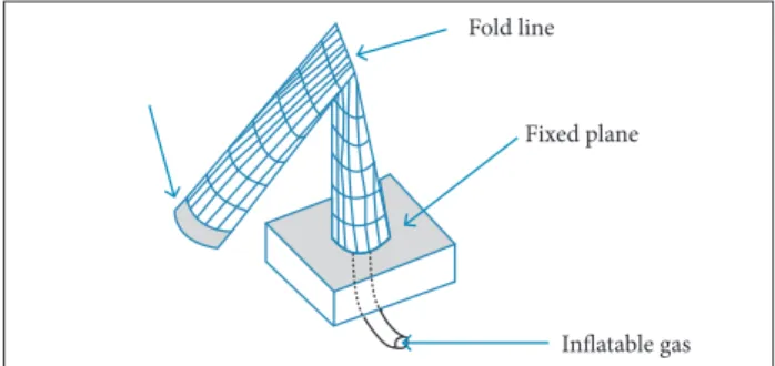
Inlatable gas Fixed plane Fold line
Figure 7. Self-contact element between the mass A and the element IJK.
Figure 8. Components of the experimental model.
he normal vector of the element plane IJK can be deined as follows:
XJI = XJ - XI, XKI = XK - XI, XKJ = XK - XJ
v3 = XJI x XKI, n = v
3/||v3|| = (xn, yn, zn)
(12)
(15)
(13)
where:
n: unit normal vector.
he equation of the element plane IJK is given as follows: Given the vectors XI, XJ, XK that describe the current position
of the nodes in the global coordinate system, the boundary vectors of the triangular element can be deined as follows:
he projected node Aʹ of mass A onto the plane is obtained by solving the following equations:
We determine whether the projected node Aʹ lies in the triangular ield by the following method.
A radial line is drawn from node Aʹ that is parallel to the ox-axis of the local coordinate system. he radial line intersects the boundary of the triangular element. If there is an odd number of intersection points, then the node Aʹ lies within the triangular ield; otherwise the node Aʹ does not lie within the triangular ield.
If the projected node Aʹ lies within the triangular element ield, there is a contact relationship between the mass A and the element IJK. When the distance from the mass A to the element IJK is less than the Euclidean distance, a penalty force is added to the mass A.
he penalty force for the mass A is deined next.
When the mass A is on the obverse side of the plane IJK, the penalty force is given as follows:
nx = (X - XI) = 0 (14)
where:
X: position vector of a random node in the plane.
(16)
When the mass A is on the reverse side of the plane IJK, the penalty force is given as follows:
Substituting Eq. 20 into Eq. 19, one yields:
where:
Fp: penalty force vector for the mass A; Cp: penalty coeicient;
kcontact: interface contact stifness which depends on the membrane
material property; hj : current distance from the mass A to the element plane IJK; h*j : ixed value for the self-contact problem; n: unit normal vector.
If the projected node Aʹ does not lie within the triangular element field, there is no contact between the mass A and the element IJK.
EQUATION OF MOTION
he equation of motion for the spring-mass system subjected to internal and external forces is given as follows:
where:
M and C: mass and damping matrices, respectively;
FI: inertial force arising from the springs; FE: generalized external force associated with the degrees of freedom of the model;
x: position vector of all the mass points.
he following equation can be written for each mass:
Let us deine the following terms:
(18)
(23)
(24) (19)
(21)
(22) (17)
j – 1 m
where:
m: mass of each mass point; c: damping of each mass point; Fex: inertial force subjected on each mass point; Fin:generalized external force subjected on each mass point.
he inite diference method can be used to simplify the two terms on the let-hand side of Eq. 19:
hen, we can write the following expression for the entire spring-mass system:
he initial coniguration of the system corresponds to a static state. hus, the displacement, the velocity and the acceleration at time 0 are zero.
In the deployment process, the initial coniguration is the folded coniguration S0 of the inlatable structures. he structures are deployed into the coniguration Si by a generalized external force. Eq. 8 is used to compute the distortion and the internal force of each spring. A penalty force is added to each of the masses in which self-contact is about to occur. Eqs. 20 and 23 are then used to calculate the values of the velocity, the acceleration and the displacement at this time; these values are added to the coniguration Si to obtain the new coniguration Si+1.
DEPLOYMENT SIMULATION SCHEME
A simple computational scheme is in the deployment mechanism simulation. his scheme is summarized next.
• he geometric parameters of the unstressed coniguration and the material parameters of membranes and cables are inputted.
• Folded methods are designed, and the initial folded configuration of the entire structure is modeled parametrically.
• he spring-mass system is formulated to describe the membrane material.
• The deployment driving forces are calculated and applied to the spring-mass system.
• he self-contact between each mass and each membrane element is determined, and a penalty force is added to each of the masses at which self-contact is about to occur.
• he boundary conditions are applied, and the equation of motion is solved using the inite diference method.
• he conigurations during the deployment process are obtained and saved as an AVI video ile.
• The deployment mechanism of the entire process and the structural performance of the fully deployed coniguration are evaluated.
he aforementioned simulation scheme is used to formulate the deployment simulation code for the inlatable antenna structures that is compiled in Fortran, and the sotware interface is compiled in MFC and OpenGL. he sotware consists of a pre-process module, a solver module and a post-pre-process module. In the pre-process module, the material and geometric parameters are inputted, and the parametric model code is run. he numerical model of the folded coniguration is then displayed graphically. Ater the numerical model of folded coniguration is veriied, the solver code is called, and the progress of the analysis process is shown. he analysis results can be opened in the post-process module. he formats of the analysis result iles are .dxf, .avi and .txt. he deployed conigurations and the fully deployed coniguration are displayed by the visualization module and are subsequently analyzed to evaluate the deployment mechanism.
NUMERICAL EXAMPLES
Z-FOLD PATTERNhe developed simulation sotware is validated by simulating a cylindrical inlatable tube that is folded in half: the results
are compared to the analysis and experimental results from Miyazaki and Uchiki (2002). Each part of the deployment experimental model for this tube is shown in Fig. 8. he bottom end of the tube is ixed, and a rigid column is attached to the tip of the tube. he initial folded coniguration of the model in the simulation is shown in Fig. 9.
Y
X Z
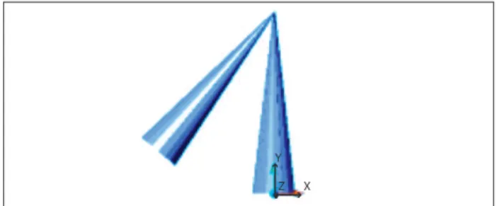
Figure 9. Folded coniguration of the model.
he experiment is conducted under micro-gravity conditions, and the atmospheric pressure is maintained at 1.03 kPa. he tube has a section radius of 12 mm and a length of 200 mm. he membrane has a thickness of 104 μm, an elastic modulus of 1.08 x 10⁸ N/m2, a Poisson’s ratio of 0.3 and a density of 910 kg/m3. he inlatable gas is nitrogen, the experimental temperature is 300.68 K, and the gas constant is 296.798 J/kgK. he shell of the rigid column has a mass of 75.7 g, a section radius of 5 mm and a thickness of 30 mm.
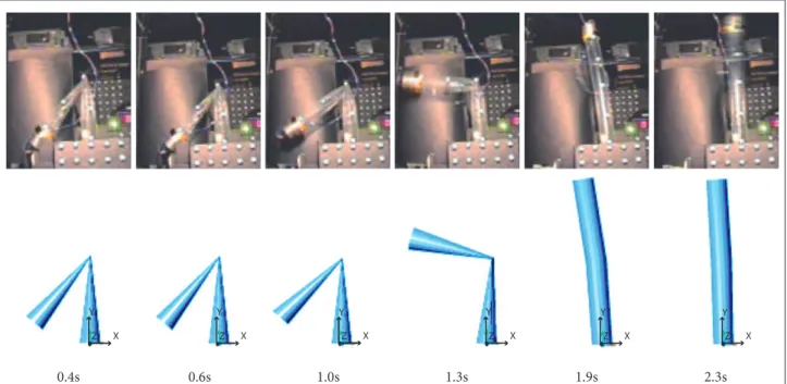
The deployment mechanism of this tube model is simulated using the developed simulation sotware to obtain the conigurations during the deployment process, which is illustrated in Fig. 10. he simulation results for the deployment process are in good agreement with the experimental results.
he internal chamber of the tube is divided into a bottom and a top compartment. he variations in the pressures in the two compartments with the deployment time are estimated using Eq. 9 and are shown in Fig. 11. Initially, the pressure in the bottom compartment increases, and the section between the two compartments is opened at a time of 0.9 s. he gas then enters the top compartment, and the pressure increases. Finally, the pressure in the two compartments reaches the design pressure of 31 kPa. Figure 12 shows that the folded angle between the two compartments changes with the deployment time. he folded angle is initially 40 degrees and increases ater 0.9 s. Finally, the tube straightens, and the folded angle reaches 180 degrees.
Figure 12. Folded angle between two compartments.
2.4 3.2
40 60 80 100 120 140 160 180
0.0 0.8 1.6
F
o
ld
ed a
n
g
le [d
eg]
Time [s]
Simulation Experiment
Infl
ata
b
le p
ress
ur
e [kP
a]
Times [s]
Figure 11. Changes in inlatable pressure.
Figure 13. Coordinates at the top end of the tube. (a) X-coordinate; (b) Z-coordinate.
Z-c
o
o
rdina
ti
o
n [m]
X-c
o
o
rdina
ti
o
n [m]
Simulation Experiment Simulation Experiment
Time [s]
Time [s]
2.4 3.2
1.6 0.8
0.0
2.4 3.2
1.6 0.8
0.0
0.00 0.05 0.10 0.15 0.20 0.25 0.05
0.00 0.10
(a)
(b)
Figure 10. Comparison between experimental and simulation results.
Y X Z Y
X Z Y
X Z Y
X Z Y
X Z
Y X Z
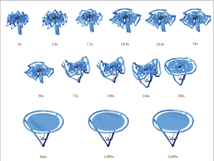
Figure 14. Individual deployment conigurations.
Z X
Y Y ZX Y ZX
COMPLETE ANTENNA MODEL
A complex inlatable antenna structure similar to that in the IAE is analyzed and modeled. he model includes inlatable tubes, an inlatable torus, a relector and tension cables. he support structure for the inlatable antenna structure consists of three tubes and a torus. here are 24 tension cables between the relector and the support structure. he geometric parameters of the unstressed coniguration are given here. he caliber D of the relector is 6 m, and the focus length f is 7.5 m. he same equation is used for the relector surface as for the canopy. he length of a single tube is 8.0498 m, and the section radius is 0.06 m. he outer diameter of the torus is 7.5 m, and the inner diameter is 7.0 m. he section radius of the torus is 0.125 m.
The membrane of the tubes, the torus and the reflector is made of Kapton. he membrane has an elastic modulus of 3.5 GPa, a Poisson’s ratio of 0.35, a thickness of 0.127 mm, and a density of 1,450 kg/m3. he tension cables are made of Kevlar
and have a diameter of 1.2 mm. he elastic modulus of Kevlar is 131 GPa. he torus has 288 elements and 144 nodes. he relector has 720 elements and 362 nodes. Each tube has 48 elements and 30 nodes. hus, the entire model has 1,152 elements and 596 nodes.
The reflector has a folded ratio of 0.5 in the longitudinal direction. The circumferential direction of the reflector and the torus are divided into 24 parts, i.e. the fold number n = 24. The radius of the torus axes curve in the folded configuration is 1.8 m. The tube is divided into four parts lengthwise and is folded using a Z-fold pattern. The entire antenna is stowed into the volume of a cylinder with a radius of 2 m and a height of 2.6 m. The design pressures of the torus and the tubes are 23.6 kPa, and the design pressure of the reflector is 100 Pa. The tubes, torus and reflector have 4, 24 and 1 inflated compartments, respectively.
he bottom point of the three tubes is connected to the satellite and remains ixed during the deployment process.
Z X Y
Z X Y
Z X Y
Z X Y
Z X Y
Z X Y
Z X Y
Z X Y
Z X Y
Z X Y
Z X Y
18s
36s
360s 1,080s 3,600s
0s
72s 3.6s
108s 7.2s
144s 10.8s
Several configurations during the deployment process are shown in Fig. 14. First, the tube and torus are inlated. he tube straightens, which causes the torus and the relector to move along the positive Z-coordinate. he cables cause the relector to move. he axes of the torus tend to form a triangular shape, which is initially driven by the three tubes and then slowly deployed into a circle curve.
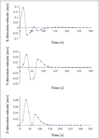
he results of the deployment dynamic simulation show that the three tubes and the axes of the torus are fully deployed at 360 s. he 3-D deployment velocities of the joint between the tube and the torus are shown in Fig. 15. At this time, wrinkles can be observed along the section direction of the torus. he relector is pulled by the tension cables, but many wrinkled regions in the relective surface remain. he relector and the torus section continue to be deployed ater 360 s. he torus section is fully deployed at 1,080 s. The reflector is slowly subjected to the design pressure and moves from its initial folded coniguration to its inal coniguration. he internal force in the relector surface is then transferred to the torus by the tension cables. he results show that the elastic deformation of the torus is very small.
The simulation results are used to evaluate the deployment dynamics of the antenna. The deployment process takes 3,600 s. The torus has a large diameter of 7.5052 m and a small diameter of 7.0855 m. The length of each tube is 8.0429 m. The fully deployed configuration has a high shape precision. Over the whole deployment process, the entire antenna structure moves smoothly from the folded configuration into the final design configuration. The results also validate the efficiency of the folded methods and the deployment mechanism simulation software of the inflatable structures.
CONCLUSION
Parametric model methods and simulation sotware for the deployment mechanism of inlatable antenna structures are investigated in this study. The unstressed and folded conigurations of the entire structure are modeled parametrically. he time histories of the structural coniguration during the deployment process and the dynamic parameters of each node are thus obtained by the simulation work. Numerical examples are used to validate the simulation sotware and the folded methods for inlatable structures. he results show that the entire antenna can be smoothly deployed from its initial folded
Figure 15. Deployment velocities of the joint between the tube and the torus.
Time [s]
Time [s]
Z-dir
ec
ti
o
n v
el
o
ci
ty [m/s]
Y
-dir
ec
ti
o
n v
el
o
ci
ty [m/s]
X-dir
ec
ti
o
n v
el
o
ci
ty [m/s]
Time [s] 0.2
0.15
0.1 0.05
0
0 50 100 150 200 250 300
0 50 100 150 200 250 300
0 50 100 150 200 250 300 350
-0.05
-0.1
0.03
0.02
0.01
0.08
0.06
0.04
0.02
0 -0.01
-0.02 -0.03 0
coniguration into the inal fully deployed coniguration. he shape of the fully deployed coniguration is in good agreement with the design coniguration.
In the present study, the number of elements used in the numerical model is not very large. he number of elements should be increased to verify the convergence of the numerical simulation. he primary members, such as the tubes and the torus, can be assembled to form complicated inlatable structures such as solar arrays and light shields. Assembly techniques for the parametric model design of the folded coniguration should be studied in the future.
ACKNOWLEDGEMENTS
REFERENCES
Bouzidi, R., Buytet, S. and Van, A.L., 2013, “A Numerical and Experimental Study of the Quasi-Static Deployment of Membrane Tubes”, International Journal of Solids and Structures, Vol. 50, No. 1, pp. 651-661. doi: 10.1016/j.ijsolstr.2012.10.027
Capua, M.D., Akin, D.L. and Davis, K., 2011, “Design, Development, and Testing of an Inlatable Habitat Element for NASA Lunar Analogue Studies”, AIAA-2011-5044, pp. 1-20.
Clem, A.L. and Smith, S.W., 2000, “A Pressurized Deployment Model for Inlatable Space Structures”, AIAA-2000-1808, pp. 1-11.
Cliff, E.W. and Ron, C.S., 2001, “A Hybrid Inlatable Dish Antenna System for Spacecraft”, AIAA-2001-1258, pp. 1-9.
David, L., 2003, “Inlatable Deployed Membrane Waveguide Array Antenna for Space”, AIAA-2003-1649, pp. 1-7.
Fang, H.F., Liu, M.C. and Hah, J., 2006, “Deployment Study of a Self-Rigidizable Inlatable Boom”, Journal of Spacecraft and Rockets, Vol. 43, No. 1, pp. 25-30. doi: 10.2514/1.3283
Haug, E., Protard, J.B. and Gerren, A.M., 1991, “The Numerical Simulation of the Inlation Process of Space Rigidized Antenna Structure”, Proceedings of the International Conference: Spacecraft Structures and Mechanical Testing, ESA, Zurich, Switzerland, pp. 862-868.
Katsumata, N., Natori, M.C. and Yamakawa, H., 2014, “Analysis of Dynamic Behavior of Inlatable Booms in Zigzag and Modiied Zigzag Folding Patterns”, Acta Astronautica, Vol. 93, No. 1, pp. 45-54. doi: 10.1016/j.actaastro.2013.06.008
Kramer, R.M.J., Cirak, F. and Pantano, C., 2013, “Fluid-Structure Interaction Simulations of a Tension-Cone Inlatable Aerodynamic Decelerator”, AIAA Journal, Vol. 51, No. 7, pp. 1640-1656.
Lampani, L. and Gaudenzi, P., 2010, “Numerical Simulation of the Behavior of Inlatable Structures for Space”, Acta Astronautica, Vol. 67, No. 3, pp. 362-368. doi: 10.1016/j.actaastro.2010.02.006
Miyazaki, Y. and Uchiki, M., 2002, “Deployment Dynamics of Inlatable Tube”, AIAA-2002-1254, pp. 1-10.
Salama, M., Fang, H.F. and Lou, M.C., 2001, “Resistive Deployment of Inlatable Structures”, AIAA-2001-1339, pp. 1-9.
Wang, C.C.L., Smith, S.S.F. and Yuen, M.M.F., 2002, “Surface Flattening Based on Energy Model”, Computer-Aided Design, Vol. 34, No. 11, pp. 823-833.
Wang, J.T. and Johnson, A.R., 2002, “Deployment Simulation of Ultra-Lightweight Inlatable Structures”, AIAA-2002-1261, pp. 1-14.
Wei, J.Z., Tan, H.F., Wang, W.Z. and Cao, X., 2015, “Deployable Dynamic Analysis and On-Orbit Experiment for Inlatable Gravity-Gradient Boom”, Advances in Space Research, Vol. 55, No. 2, pp. 639-646. doi: 10.1016/j.asr.2014.10.024
Xiao, X., Guan, F.L. and Xu, Y., 2010, “Numerical Analysis and Experimental Study on Deployment Process of Coil-Folded Inlatable Tube” (in Chinese), Journal of Zhejiang University (Engineering Science), Vol. 44, No. 1, pp. 184-189.
Xu, Y., Guan, F.L., Chen, J.J. and Zheng, Y., 2012, “Structural Design and Static Analysis of a Double-Ring Deployable Truss for Mesh Antennas”, Acta Astronautica, Vol. 81, No. 2, pp. 545-554. doi: 10.1016/j.actaastro.2012.09.004