www.hydrol-earth-syst-sci.net/18/1539/2014/ doi:10.5194/hess-18-1539-2014
© Author(s) 2014. CC Attribution 3.0 License.
Hydrology and
Earth System
Sciences
Climate information based streamflow and rainfall forecasts for
Huai River basin using hierarchical Bayesian modeling
X. Chen1,6, Z. Hao1, N. Devineni2,3, and U. Lall4,5
1State Key Laboratory of Hydrology-Water Resources and Hydraulic Engineering, Hohai University, Nanjing 210098, China 2Department of Civil Engineering, The City University of New York (City College), New York, NY 10031, USA
3NOAA-Cooperative Remote Sensing Science and Technology Center, The City University of New York (City College),
New York, NY 10031, USA
4Columbia Water Center, The Earth Institute, Columbia University, New York, NY 10027, USA
5Department of Earth and Environmental Engineering, Columbia University, New York, NY 10027, USA 6Bureau of Hydrology, Changjiang Water Resources Commission, Wuhan 430010, China
Correspondence to:N. Devineni ([email protected])
Received: 22 July 2013 – Published in Hydrol. Earth Syst. Sci. Discuss.: 12 September 2013 Revised: 8 March 2014 – Accepted: 14 March 2014 – Published: 29 April 2014
Abstract.A Hierarchal Bayesian model is presented for one season-ahead forecasts of summer rainfall and streamflow using exogenous climate variables for east central China. The model provides estimates of the posterior forecasted proba-bility distribution for 12 rainfall and 2 streamflow stations considering parameter uncertainty, and cross-site correlation. The model has a multi-level structure with regression coef-ficients modeled from a common multi-variate normal dis-tribution resulting in partial pooling of information across multiple stations and better representation of parameter and posterior distribution uncertainty. Covariance structure of the residuals across stations is explicitly modeled. Model per-formance is tested under leave-10-out cross-validation. Fquentist and Bayesian performance metrics used include re-ceiver operating characteristic, reduction of error, coefficient of efficiency, rank probability skill scores, and coverage by posterior credible intervals. The ability of the model to re-liably forecast season-ahead regional summer rainfall and streamflow offers potential for developing adaptive water risk management strategies.
1 Introduction
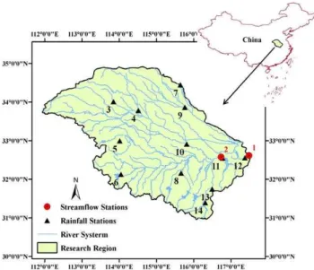
The Huai River basin (Fig. 1), located between the Yangtze and Yellow River basins is the most densely inhabited river basin and the main cropping area in China. The total drainage
area of 270 000 km2is divided into the Huai River catchment (190 000 km2)and the Yishusi River catchment (80 000 km2) by a paleo-channel of Yellow River. The mean annual precip-itation for the Huai River basin is approximately 900 mm, of which 50–75 % occurs during the summer monsoon season. There are 36 large reservoirs in the basin primarily designed for water supply and flood control (Zhang et al., 2012). Nat-ural climate variations in conjunction with increasing popu-lation demands are causing severe water stress in the region. Moreover, the region is susceptible to droughts and floods with a recurrent frequency of four years on average (Yan et al., 2013; Cheng et al., 2012). Such variations in water sup-ply are often related to inter-annual fluctuations in large-scale climatic patterns. In this paper, potential climate teleconnec-tions are explored and formalized into a predictive model in a Bayesian framework which allows for formal uncertainty reduction and modeling. Applications for water, food and en-ergy management using such probabilistic forecasts could be developed as part of a strategy for climate risk mitigation and for adaptation to a variable climate.
Fig. 1.Location of the study area.
statistical downscaling to develop regional hydrologic fore-casts (Robertson et al., 2004; Gangopadhyay et al., 2005). Alternately, one can develop a low-dimensional statistical model by relating the observed rainfall or streamflow to iden-tified climatic precursors (e.g., El Ninõ–Southern Oscillation (ENSO) indices) for the given site (Souza and Lall, 2003). A key aspect in developing such dynamic or statistical models is the ability to accurately represent the uncertainties, both at the model representation level and at the parameter estima-tion level. Developing statistical schemes that can address si-multaneous prediction at multiple sites and for multiple vari-ables while addressing their correlation structure is often a challenge.
Hierarchical Bayesian methods provide the opportunity to explicitly quantify the parameter uncertainty through each estimation stage using appropriate conditional and prior dis-tributions. This allows a better representation of model and parameter uncertainties. Recently, Devineni et al. (2013) pre-sented a hierarchical Bayesian regression strategy for esti-mating streamflow at multiple locations using various model structures to pool information across multiple sites to an ap-propriate degree such that the features that are common to the site regression and those that vary across sites can be identified for an overall reduction in parameter uncertainty while preserving the structure in errors across the stations. Here, a similar Hierarchical Bayesian approach is developed for regional rainfall and streamflow forecasts using appropri-ate climappropri-ate indicators that could be derived from GCMs or observed climate fields. The application focuses on the up-per and middle regions of the Huai River basin which are of interest for local management, and may have similar cli-matic forcing. Section 2 provides a brief description of the study area, data sources and the climate predictor identifica-tion procedure. The hierarchical Bayesian regression model
2 Data description
2.1 Streamflow and rainfall data
We used streamflow data from two stations and rainfall data from 12 stations in this study to develop regional hydro-logic forecasts. The streamflow data are from the Bengbu (117.38◦
E, 32.56◦
N) and the Lutaizi (116.79◦
E, 32.57◦
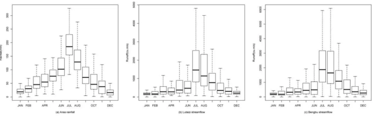
N) hydrological stations (shown as red dots in Fig. 1). Twelve rainfall stations with at least 50 years of data were selected in the contributing section of the basin (shown as filled triangles in Fig. 1). The details of the hydrologic stations including the number of years of data records are shown in Table 1. Prelim-inary analysis of the seasonality of streamflow and area aver-aged rainfall show that more than 50 % of the annual rainfall and streamflow occurs in June-July-August (JJA) (Fig. 2). Consequently, a prediction of the summer monsoon rainfall and streamflow in June or earlier is of interest.
2.2 Climate teleconnection and predictor identification
Xu et al. (2007) and Kwon et al. (2009) developed season-ahead streamflow forecasts for the Yangtze River on the Three Gorges Dam using exogenous climate indices from eastern Indian Ocean and western Pacific Ocean. Recently, Liu et al. (2013) and Linderhorm et al. (2013) investigated the relation between East Asian monsoon rainfall and North Atlantic sea surface temperature conditions using observa-tions and paleo-reconstructed records. So far little work has been done for climate informed hydrologic prediction for the Huai River basin. To identify predictors that influ-ence the regional hydroclimate in the basin during JJA sea-son, we consider SST anomaly conditions during February-March-April (FMA, 3 months lag) and October-November-December (OND, 6 months lag) obtained from the Hadley Center SST dataset (HADSST2) (Rayner et al., 2006). Fig-ure 3 shows the Spearman’s rank correlation between the observed streamflow during JJA at the Bengbu hydrologic station and the pre-season SST conditions. The 3-month lag correlation (i.e., JJA streamflow with FMA SSTa) and the 6-month lag correlation (i.e., JJA streamflow with OND SSTa) are shown in Fig. 3a and b, respectively. From Fig. 3a, we see that the SST1 region (155–175◦E and 40–50◦N)
Fig. 2.Seasonality of area rainfall and streamflow in study region.
Table 1.Detail information for streamflow and rainfall station used in this study.
Station Station Elevation Actual data record ID name Abbreviation (m) Category & used for reconstruction
1 Bengbu BB 10.0 streamflow 1951–2010 2 Lutaizi LTZ 19.0 streamflow 1951–2010 3 Xuchang XC 66.8 rainfall 1952–2010 4 Xihua XH 52.6 rainfall 1955–2010 5 Zhumadian ZMD 82.7 rainfall 1958–2010 6 Xinyang XY 114.5 rainfall 1951–2010 7 Shangqiu SQ 50.1 rainfall 1953–2010 8 Gushi GS 57.1 rainfall 1952–2010 9 Bozhou BZ 37.7 rainfall 1953–2010 10 Fuyang FY 30.6 rainfall 1953–2010 11 Shouxian SX 22.7 rainfall 1955–2010 12 Bengbu BB 18.7 rainfall 1952–2010 13 Liuan LA 60.5 rainfall 1956–2010 14 Huoshan HS 68.1 rainfall 1954–2010
above-normal inflow conditions in the Huai River. Similarly, from Fig. 3b, we can see that 6-month prior conditions in the North Atlantic Ocean identified as SST2 (15◦
W–5◦
E and 35–55◦
N) influence the summer flows in the basin. This is in line with an earlier finding (Gu et al., 2009a) which showed that the East Asian summer monsoons are strongly related to a tripole mode of the North Atlantic SST anomalies in the preceding winter that typically enhances the stationary wave-train propagating from west Eurasia to East Asia. The correlations with SST1 and SST2 are statistically significant at the 95 % level.
In addition to the SST anomaly conditions, we also con-sidered the 4-month lagged (February-March-April) North Atlantic oscillations (NAO) (Hurrell et al., 2003), summer North Atlantic oscillation (SNAO) (Folland et al., 2009) and 6-month lagged (November-December-January) Atlantic Multi-decadal Oscillation (AMO) (Knight et al., 2006) as candidate predictors. Gu et al. (2009b) showed that the Jan-uary and March NAO modulates the summer rainfall patterns over China. Following Linderholm et al. (2011), we selected the SNAO as one of the predictors as it influences the storm
tracks over China with wetter than normal conditions dur-ing positive SNAO phase and drier than normal conditions during negative phase. Similarly, AMO has been shown as an important covariate for climate in central Asia with pos-itive AMO phase leading to strong southeast summer mon-soons and late retrieval (Lu et al., 2006). We also checked the relationship between ENSO indices, Pacific decadal os-cillation and the Northern Hemisphere snow cover with sum-mer streamflow and rainfall in the basin. There was no sta-tistically significant correlation between these covariates and streamflow or rainfall in the region. Table 2 summarizes the correlations between the two streamflow stations, area aver-aged rainfall and the climate predictors selected for the study.
3 Methodology
3.1 Hierarchical Bayesian model
SST1 SST2 AMO NAO SNAO
Lutaizi 0.44 (FMA) 0.45 (OND) 0.28 (NDJ) −0.26 (FMA) 0.39 (FMA) Bengbu 0.44 (FMA) 0.47 (OND) 0.21 (NDJ) −0.22 (FMA) 0.34 (FMA) Area rainfall 0.46 (FMA) 0.51 (OND) 0.36 (NDJ) −0.27 (FMA) 0.36 (FMA)
∗() is the selected period of the predictor for streamflow prediction; Area rainfall is the average rainfall of 12 stations in the study region.
Fig. 3.SST regions (SST1 and SST2) that influence the rainfall and streamflow in the Huai River basin. SST regions that have signif-icant correlation at 95 % confidence interval (>0.25 or<−0.25) are considered as predictors for the hierarchical Bayesian model. (SST1: 40–50◦N, 155–175◦E; SST2: 35–55◦N, 15◦W–5◦E).
streamflow and rainfall. The basic idea is that a particu-lar climate predictor may inform the rainfall or streamflow anomaly at each of the sites in the region in a similar way. If the response were exactly the same, predicting the average of the station values or pooling all the data into the same regression would be effective since that would reduce the uncertainty associated with parameter estimation. However, the response across the rainfall and the streamflow stations may vary systematically due to local conditions or averag-ing scale (e.g., for a large river basin vs. small or point rain-fall). The hierarchical model can be used for partial pooling of this common information, by considering multiple levels of modeling. The individual regression coefficients for each site on each climate predictor are estimated at the first level.
The second level estimates the average regression coefficient across sites and its variance, thus allowing variation in the response across sites, but also its potential shrinkage to an appropriate degree through an estimation of the variance. If the variance estimated is large, then the model tends towards a model that would be formed if each site was regressed inde-pendently on the predictor. If the variance is small, then the model tends towards a fully pooled regression model, and the responses are deemed homogeneous. Partial pooling reduces the equivalent number of independent parameters, resulting in lower uncertainty in parameters estimates, and therefore reduced uncertainty in the final forecasts. The general mod-eling framework is presented as follows.
and the priors associated with the parameters and the hyper-parameters are presented below:
Level 1: log(Yt)∼N µt,6
(1)
µit=αi+Xtβ (2)
Level2: β∼ MVN(µβ,6β). . . (3) With priors modeled as
αi ∼N (0,10000) µβ∼N (0,10000) 6β∼Inv-Wishartv0(30)
6∼ Inv-Wishartv1(31) (4)
The prior for the covariance matrix 6β is taken to be the inverse Wishart distribution with a scale matrix30 andν0
degrees of freedom. In our applications, the scale matrices 30and31 were specified as an identity matrix (I) and the
degrees of freedom ν0 and ν1 were set to one more than
the dimension of the matrix (i.e., the total number of pre-dictors, five for6β and total number stations, 14 for6)to induce a uniform prior distribution on the variance (Gelman and Hill, 2007). This choice of priors was made for computa-tional convenience and represents a simpler model than could be formulated if all parameter covariance were to be mod-eled. The joint posterior distributionp(θ|data), of the com-plete parameter vectorθ is derived by combining the prior distributions and the likelihood functions. The parametersθ are estimated using WinBUGS (Spiegelhalter et al., 1996) which employs the Gibbs sampler, a Markov chain Monte Carlo (MCMC) method for simulating the posterior proba-bility distribution of the parameters conditional on the cur-rent choice of parameters and the data. A discussion on such model constructs and their comparison to a no pooling model that estimates independent regressions across sites and to a full pooling model that ignores the cross-site variations in re-sponse is presented in Devineni et al. (2013). Several hydro-logic applications using Bayesian model constructs have also been developed and demonstrated in Lima and Lall (2009, 2010), and Kwon et al. (2008). Renard et al. (2013) present a useful tutorial and examples of related Bayesian models for hydroclimatic applications.
3.2 Cross-validation
Cross-validation statistics computed over different blocks of data can reveal how well the Bayesian model can perform in truly out of sample predictions recognizing that differ-ent climate epochs may lead to differdiffer-ent model fits and per-formance. We evaluate the model using an m-fold cross-validation technique. A sample is formed by leaving outm randomly selected data points from the observational data set for validation and the Bayesian model is developed using the remaining(n−m)observations. This process is repeated sev-eral times to obtain an ensemble of validation metrics result-ing from each randomly selected model. In the applications
presented in the later section,mwas 10,n was 50, and 30 sample models were fit. We use three traditional performance metrics, reduction of error (RE) and coefficient of efficiency (CE) and the rank probability skill score (RPSS), as mea-sures of model performance to compare the forecasted pos-terior mean and the distribution of the streamflow and rainfall estimates with the actual streamflow and rainfall data.
The reduction of error (RE) ranges from−∞to+1 and is similar to theR2statistic (Lorenz, 1956; Fritts, 1976).
RE=1.0− n P
t=1
(Ot−St)2 n
P
t=1
(Ot−oc)2
(5)
In Eq. (5),Ot andSt are the observed and the predicted pos-terior mean of the streamflow (transformed back to real space by taking anti-logs) in yeartof the validation period andocis
the mean of the observational data in the calibration period. RE>0 indicates that the simulated streamflow contains use-ful information not contained in the calibration period. Sim-ilarly RE<0 indicates that the simulations are poorer than climatology, i.e., the simulations are not better than the mean flows in the calibration period. The coefficient of efficiency (CE) is defined as
CE=1.0− n P
t=1
(Ot−St)2 n
P
t=1
(Ot−ov)2
. (6)
In Eq. (6),Ot andSt are the observed and the predicted pos-terior mean of the streamflow in yeart of the validation pe-riod andovis the mean of the observational data in the
valida-tion period. CE<0 indicates that the simulations are poorer than validation climatology, i.e., the simulations are not bet-ter than the mean flows in the validation period. CE is similar to RE, but used as a measure to evaluate the model under the validation period, it is a more rigorous metric.
In addition to RE and CE that measure the error in predict-ing the conditional mean, we also verify the RPSS to quan-tify the error in estimating the entire probability distribution of the forecast (Wilks, 2011; Candille and Talagrand, 2005; Gangopadhyay et al., 2005). The RPSS is based on the rank probability score (RPS) computed for each forecast and ob-servation pair at each station in each year:
RPS= n X
k=1
(Sk−Ok)2, (7)
whereSkis the cumulative probability of the forecast for
cat-egory k andOkis the cumulative probability of the
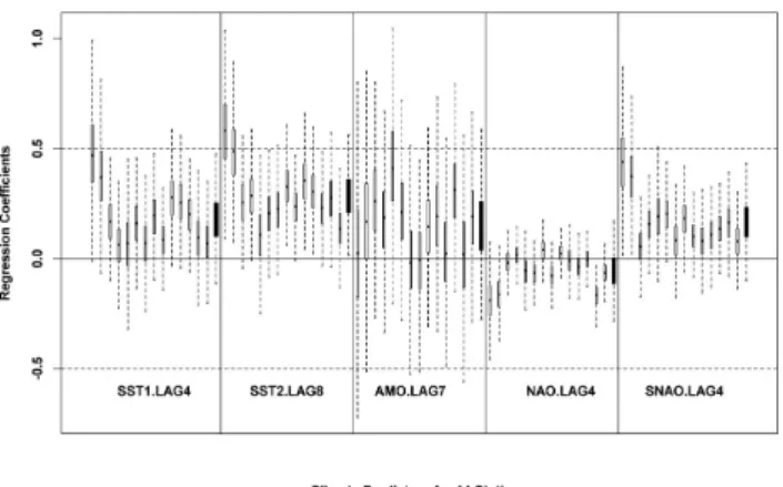
β µβ
Fig. 4.Box plots of the regression coefficientsβij (open box) and theµβj mean of the regression coefficients (filled box) for the five predictors. The first two box plots for each predictor correspond to the streamflow stations and the next 12 to the rainfall stations.
values. These categories are determined separately for each station in the basin. Next, for each forecast at each station and year, the cumulative probability associated with each of the k categories is assessed by counting the fraction of the 1000 ensemble members from the hierarchical Bayesian regres-sion model for that year for that station. Correspondingly, for each year and station, the observed cumulative probabil-ities for each category are assigned as 0, if k<k*, and 1 if k≥k*, where k* is the category in which the observation for that year and station falls.
Now the RPS is computed as the squared difference be-tween the observed and forecast cumulative probabilities, and the squared differences are summed over all three cat-egories. The RPSS is then computed as
RPSS=1− RPSforecast RPSclimatology
, (8)
where RPSforecast is the mean ranked probability score for
model forecast and RPSclimatologyis the mean ranked
proba-bility score for climatological forecast. RPSS represents the level of improvement of the forecast in comparison to ref-erence forecast which is usually assumed to be climatology. Similar to RE and CE, an RPSS>0 indicates that the fore-casts have skill better that the climatology, and vice versa.
4 Results and discussion
The posterior distribution of the regression coefficients (β) for each climate predictor and the mean of the vector of regression coefficients across sites (µβ)from the joint nor-mal distribution, is shown in Fig. 4 through box plots of the values simulated from the posterior density functions. All the predictors except NAO have positive coefficients for the mean response across sites. Note that the spread on each µβ covers the median of the 14 correspondingβs, as would
from those for rainfall. This is expected given that the stream-flow represents a spatial averaging of the rainfall process, and hence may have lower uncertainty and better identifiability. One could consider modeling these as separate groups to be pooled. However, given that we have only 2 streamflow sta-tions, pooling across them would not provide much improve-ment in this application. Modeling them together provides a larger sample size (14) for the estimation of the coefficients of the Level 2 model, and leads to a higher spread in the posterior distribution ofµβ than would result if we modeled the rainfall and streamflow stations in separate groups. An averaging of a larger number of rainfall stations with stream-flow stations that individually represent a spatial averaging of rainfall is attractive from a conceptual perspective to regular-ize or reduce the uncertainty in the estimates of the response for the noisier rainfall stations. The simulations of the co-variance matrix across predictors,6β (results not shown), have non-zero off-diagonal elements. If two predictors are highly correlated then their regression coefficients cannot be uniquely identified through classical or Bayesian regression. However, their mean and covariance can be estimated and simulations of the log(Y) generated from the Bayesian model would be based on this covariance across the associated re-gression coefficients. Hence, an appropriate range of log(Y) values will be generated for each prediction, even though the individualβare not uniquely identified due to predictor cor-relation.
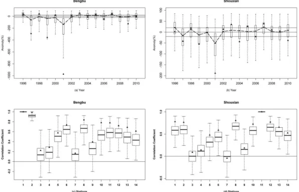
The posterior probability distributions of the forecasts from the model for the streamflow at Bengbu station and rainfall at Shouxian station during the period 1996–2010 are shown as box plots in Fig. 5a and b, respectively. While the Bayesian model is developed using all the data, the fore-casts are shown for the last 15 years to make a cleaner fig-ure. Subsequent performance metrics are evaluated under cross-validation. The plots show streamflow and rainfall val-ues as the percentage difference each year from their long-term average (1696 m3s−1for the flow at Bengbu station and
455 mm for rainfall at Shouxian). We see that the directional indication of the forecast is generally quite accurate while the uncertainty varies from year to year. We also computed the coverage rate under Bayesian credible intervals for the model and observe that for a 90 % credible interval, on aver-age, over the 14 stations, approximately 10 % of the observed data are outside the interval, indicating the robustness of the fitted model.
Fig. 5.The posterior probability distributions for JJA averaged streamflow and JJA total rainfall for(a)standardized streamflow at Bengbu station and(b)standardized rainfall at Shouxian station. The posterior distribution of the cross-site correlation for Bengbu station and for Shouxian station is presented in(c)and(d), respectively. Each box plot has the 25th, median and 75th percentile of the posterior distribution, with whiskers extended to the extreme values sampled. The solid triangle denotes the observation.
months lag predictors, the sign of a strong shift in the proba-bility will alert the decision makers to an anticipated extreme event. Decision makers are often influenced by the ability to correctly indicate extreme conditions since the losses from their operations are most sensitive to such states. In our in-teractions with corporate and public sector decision makers, we have noticed both skepticism induced by failure to pre-dict extremes, even if all performance measures are good, and conversely enthusiasm for the model on noting that the directional (high, average, low) forecasts are quite good.
However, we do see the consistent underestimation of dry conditions as evidence that either the tail behavior of the forecast distribution or the linearity of the link function be-tween the predictors and the predictands is in question. The usual tests of goodness of fit accepted the hypothesis that the log-normal distribution was a good fit to the data, but discrimination with other distributions given the sample size may well lack power. Given the relatively short records, es-pecially with our emphasis on cross-validation, and the di-mension of the predictor space, exploration of a nonlinear model across the five predictors and 14 sites, and in the gen-eral case with more sites and predictors is challenging. In upcoming work, we are considering Gaussian process mod-els (Rasmussen and William, 2006; Brahim-Belhouari and Bermak, 2004) to address this setting in a formal way.
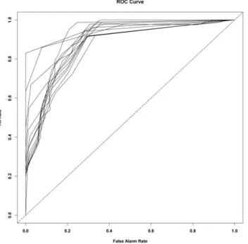
To provide insight as to how applications of the categor-ical forecasts could be approached, we present (Fig. 6) the receiver/relative operating characteristic (ROC) plot (Mason, 1982) considering the decile categorical thresholds on the forecast posterior probability distribution for each of the 14 forecasts. Forecasts with better discrimination from random chance typically exhibit a ROC curve approaching the upper-left corner of the diagram as opposed to the 45◦ diagonal
lines, where the forecast has little ability to discriminate from a 50:50 probability that occurs by chance. From Fig. 6, we see that the ROC curve for all the 14 stations is well beyond the diagonal line and approaches the left corner indicating that the forecasts exhibit hit rates higher than the false alarm rate and are well calibrated to predict anomalous events us-ing exogenous climate precursors. In reality a decision maker could prescribe their own thresholds of interest and evaluate the consequences of the forecast relative to the uncertainty and the threshold prescribed, as part of the decision process. In summary, while the conventional model checking under Bayesian modeling involves verifying for coverage rates and uncertainty level, we also verified our models using the stan-dard verification procedures used in climate forecasting from various institutions for benchmarking (Barnston et al., 2003; Goddard and Mason, 2003).
Fig. 6.ROC plot from the forecasts based on decile categorical thresholds for all the 14 streamflow and rainfall stations.
applications. Here, the spatial correlation is estimated from the posterior distribution of the streamflow and rainfall and compared to the observed cross-site correlation. The results for two stations (station1: streamflow from Bengbu station, station 11: rainfall from Shouxian station) are shown in Fig. 5c and d. The box plots in Fig. 5c and d present the posterior probability distribution of the correlations for these station with each of the 13 other stations. The observed cor-relation for each station is shown as a triangle. The fore-cast ensembles provide a good reproduction of the spatial correlation across all years.
The results for RE, CE, and RPSS performance under m-fold cross-validation for each station are shown in Fig. 7. RE and CE are used to measure the goodness of fit of the model by comparing the forecasted streamflow and rainfall with the actual observed data. They are used as an expression of the trueR2of the regression equation when applied to new data. By assessing the RE and CE under cross-validation, we are essentially providing a measure of the variance explained un-der a validation data set. Given that seasonal forecasts are better represented probabilistically using the posterior dis-tribution, expressing the skill of the forecast using RE and CE requires summarizing the forecasts using measures of central tendency such as mean or median of the posterior distribution which does not give credit to the probabilistic information in the forecasts. RPSS computes the cumula-tive squared error between the categorical forecast probabil-ities and the observed category in relevance to a reference forecast. We observe that typically the hierarchical Bayesian model leads to values of RE, CE and RPSS greater than zero
Fig. 7.Performance under “leave-10-out cross-validation” for all 14 stations from the hierarchical Bayesian model from 30 random sim-ulations –(a)reduction of error (RE),(b)coefficient of efficiency (CE),(c)Rank probability skill score (RPSS).
for all the stations (except Huoshan station −14) indicat-ing that the seasonal forecasts developed usindicat-ing the climate precursors contain useful information.
(30×10 years) forecasts. The average coverage rate across the stations is 92 % for the corresponding to the 90 % cover-age interval indicating the robustness of the fitted Bayesian models under cross-validation.
5 Summary
This study investigated the predictability of the summer rain-fall and streamflow in the upper and mid-Huai River basin using five selected large-scale climate indices as predictors. The study identified two regions, one in the North Pacific and one in the North Atlantic in addition to pre-season AMO, NAO and SNAO that can be used as climatic precursors for JJA streamflow and rainfall in the Huai River basin. As the underlying challenge is to consistently model the vari-ability across sites and across variables, we employed a hi-erarchical Bayesian model strategy. Hihi-erarchical Bayesian models and multi-level models have become quite com-mon as educational and research tools for Computational Statistics. They appear for applications in causal inference, prediction, comparison and data description especially for multi-variable problems where the investigator needs to learn something about the group as well as individual dynamics. In many cases, they directly generalize traditional regression approaches in this setting. Given our experience with such models in other contexts, we were interested in exploring how a structured approach to regional statistical forecasts of streamflow and rainfall could be approached. In general, this is a high dimensional problem that offers some interesting opportunities both from a model framing context and from a regularization context.
The partial-pooling hierarchical Bayesian regression model provided a useful way to model spatial co-variability in seasonal hydrological predictions, while considering the potentially common effects of the predictors on regional hy-drologic response. An advantage of the approach is that it al-lows appropriate grouping of information in the region, and explicit modeling of the covariance of the model errors and the regression coefficients to better represent the uncertainty in both the model parameters and the final streamflow and rainfall forecasts. Cross-validated model results show good predictive skill, and the common effects as well as the at site effects of each predictor are identified well even un-der leave-10-out of 50 cross-validation. Comparison of the partial-pooling model with a no-pooling model in the same estimation framework (equivalent to the traditional regres-sion based modeling framework) showed that the Bayesian model is competitive or superior in terms of the validation statistics. An aspect of Bayesian modeling that is often cited is the ability to provide a systematic approach to the propa-gation and modeling of model parameter uncertainty. In this context, we argue that while there could be a potential up-per limit in predictability in seasonal rainfall using anoma-lous SST conditions as shown in Westra and Sharma (2010),
from a forecast utility point of view, knowing the uncer-tainty is certainly useful since it can be used for develop-ing probability-based risk management models for optimiz-ing reservoir operations or agricultural decision models. We find this useful, but also note that typically these models re-quire assumptions as to parametric probability density mod-els. There is a practical utility especially in the context of dynamical and statistical regional forecast models to being able to generate consistent simulations across parameters and output variables and to build in a multi-level modeling struc-ture in one shot using multi-level or hierarchical models. Our future work in the region will focus on using the forecasts developed to specify dynamic rules for operating multiple reservoir systems in the basin using both multi-site seasonal hydrologic forecasts and changing demand through adaptive human behavior to better manage deficits from the reservoirs. A refinement of the method applied here to disaggregating the rain and streamflow in time over the season to prop-erly capture monsoon breaks and the amplitude, duration and spatial structure of rainfall events will be a goal for these applications. Nonlinearity and non-Gaussian aspects will be modeled in a Gaussian process framework.
Acknowledgements. We thank the Royal Netherlands Meteo-rological Institute (KNMI), hydMeteo-rological bureau of Huai River and China Meteorological Data Sharing Service System for the data used in this study. The work was funded in part by China Scholarship Council, the PepsiCo Foundation, the Columbia Water Center, the National Basic Research Program of China (grant no. 2010CB951103), Nonprofit Industry Research Special Fund of China’s MWR (201101003), National Natural Science Foundation of China (41101015, 41271042 and 41101016), the Special Fund of State Key Laboratory of Hydrology-Water Resources and Hydraulic Engineering (1069-50985512), the “Strategic Priority Research Program” of the Chinese Academy of Sciences XDA05110102. The authors would like to thank the two anonymous reviewers whose valuable comments led to significant improvements in the manuscript.
Edited by: H. H. G. Savenije
References
Barnston, A. G., Mason, S. J., Goddard, L., Dewitt, D. G., and Ze-biak, S. E.: Multimodel ensembling in seasonal climate forecast-ing at IRI, B. Am. Meteorol. Soc., 84, 1783–1796, 2003. Brahim-Belhouari, S. and Bermak, A.: Gaussian process for
non-stationary time series prediction. Comput. Stat. Data Anal., 47, 705–712, 2004.
Candille, G. and Talagrand, O.: Evaluation of probabilistic predic-tion systems for a scalar variable, Q. J. Roy. Meteorol. Soc., 131, 2131–2150, doi:10.1256/qj.04.71, 2005.
Hierarchical Bayesian Regression, J. Climate, 26, 4357–4374, doi:10.1175/JCLI-D-11-00675.1, 2013.
Fritts, H. C.: Tree rings and climate, Academic Press, London, 1976.
Folland, C. K., Knight, J., Linderholm, H. W., Fereday, D., Ineson, S., and Hurrell, J. W.: The summer North Atlantic Oscillation: past, present, and future, J. Climate, 22, 1082–1103, 2009. Gangopadhyay, S., Clark, M., and Rajagopalan, B.: Statistical
downscaling using K-nearest neighbors, Water Resour. Res., 41, W02024, doi:10.1029/2004WR003444, 2005.
Gelman, A. and Hill, J.: Data Analysis Using Regression and Mul-tilevel/Hierarchical Models, Cambridge University Press, New York, NY, 2007.
Geng, Q. Z., Ding, Y. H., and Huang, C. Y.: Influences of the Ex-tra tropical Pacific SST On the Precipitation of the North China Region, Adv. Atmos. Sci., 14, 339–349, 1997.
Goddard, L. and Mason, S. J.: Evaluation of the IRI’s “net assess-ment” seasonal climate forecasts: 1997–2001, B. Am. Meteorol. Soc., 84, 1761–1781, 2003.
Gu, W., Li, C. Y., Wang, X., and Zhou, W.: Linkage between mei-yu precipitation and North Atlantic SST on the decadal timescale, Adv. Atmos. Sci., 26, 101–108, doi:10.1007/s00376-009-0101-5, 2009a.
Gu, W., Li, C. Y., Wang, X., Zhou, W., and Chan, J. C. L.: Inter-decadal unstationary relationship between NAO and east China’s summer precipitation patterns, Geophys. Res. Lett., 36, L13702, doi:10.1029/2009GL038843, 2009b.
Hurrell, J. W., Kushnir, Y., Ottersen, G., and Visbeck, M. (Eds.): The North Atlantic Oscillation: Climatic Significance and En-vironmental Impact, Geophys. Monogr. Ser., Vol. 134, 279 pp., AGU, Washington, D. C., doi:10.1029/GM134, 2003.
Knight, J. R., Folland, C. K., and Scaife, A. A.: Climate impacts of the Atlantic Multidecadal Oscillation, Geophys. Res. Lett., 33, L17706, doi:10.1029/2006GL026242, 2006.
Kwon, H.-H., Brown, C., and Lall, U.: Climate informed flood frequency analysis and prediction in Montana using hierar-chical Bayesian modeling, Geophys. Res. Lett., 35, L05404, doi:10.1029/2007GL032220, 2008.
Kwon, H.-H., Brown, C., Xu, K., and Lall, U.: Seasonal and annual maximum streamflow forecasting using climate information: Ap-plication to the Three Gorges Dam in the Yangtze River basin, China, Hydrol. Sci. J., 54, 582–595, 2009.
Lima, C. H. and Lall, U.: Hierarchical Bayesian modeling of multi-site daily rainfall occurrence: Rainy season onset, peak, and end, Water Resour. Res., 45, W07422, doi:10.1029/2008WR007485, 2009.
Lima, C. H. and Lall, U.: Spatial scaling in a changing climate: A hierarchical bayesian model for non-stationary multi-site an-nual maximum and monthly streamflow, J. Hydrol., 383, 307– 318, 2010.
tions between the summer North Atlantic Oscillation and the East Asian summer monsoon, J. Geophys. Res., 116, D13107, doi:10.1029/2010JD015235, 2011.
Lorenz, E. N.: Empirical orthogonal functions and statistical weather prediction. MIT statistical forecasting project report no.1, contract AF 19, 604–1566, 1956.
Lu, R., Dong, B., and Ding, H.: Impact of the Atlantic Multidecadal Oscillation on the Asian summer monsoon, Geophys. Res. Lett., 33, L24701, doi:10.1029/2006GL027655, 2006.
Mason, I.: A model for assessment of weather forecasts, Aust. Met. Mag., 30, 291–303, 1982.
Rasmussen, C. E. and William, C. K. I.: Gaussian processes for machine learning, MIT Press, 2006.
Rayner, N. A., Brohan, P., Parker, D. E., Folland, C. K., Kennedy, J. J., Vanicek, M., Ansell, T. J., and Tett, S. F. B.: Im-proved Analyses of Changes and Uncertainties in Sea Sur-face Temperature Measured In Situ since the Mid-Nineteenth Century: The HadSST2 Dataset, J. Climate, 19, 446–469, doi:10.1175/JCLI3637.1, 2006.
Renard, B., Sun, X., and Lang, M.: Bayesian Methods for Non-stationary Extreme Value Analysis, in: Extremes in a Changing Climate, 39-95, Springer Netherlands, 2013.
Robertson, A. W., Kirshner, S., and Smyth, P.: Downscaling of daily rainfall occurrence over northeast Brazil using a hidden Markov model, J. Climate, 17, 4407–4424, 2004.
Souza Filho, F. A. and Lall U.: Seasonal to interannual ensemble streamflow forecasts for Ceara, Brazil: Applications of a multi-variate, semiparametric algorithm, Water Resour. Res., 39, 1307– 1319, doi:10.1029/2002WR001373, 2003.
Spiegelhalter, D., Thomas, A., Best, N., and Gilks, W.: BUGS 0.5: Bayesian inference Using Gibbs Sampling–Manual (version ii), Medical Research Council Biostatistics Unit, Cambridge, 1996. Westra, S. and Sharma, A.: An Upper Limit to Seasonal
Rainfall Predictability?, J. Climate, 23, 3332–3351, doi:10.1175/2010JCLI3212.1, 2010.
Wilks, D. S.: Statistical methods in the atmospheric sciences, Ac-cess Online via Elsevier, 2011.
Xu, K., Brown, C., Kwon, H. H., Lall, U., Zhang, J., Hayashi, S., and Chen, Z.: Climate teleconnections to Yangtze river seasonal streamflow at the Three Gorges Dam, China, Int. J. Climatol., 27, 771–780, doi:10.1002/joc.1437, 2007.
Yan, D. H., Wu, D., Huang, R., Wang, L. N., and Yang, G. Y.: Drought evolution characteristics and precipitation inten-sity changes during alternating dry-wet changes in the Huang-Huai-Hai River basin, Hydrol. Earth Syst. Sci., 17, 2859–2871, doi:10.5194/hess-17-2859-2013, 2013.