www.j-sens-sens-syst.net/4/85/2015/ doi:10.5194/jsss-4-85-2015
© Author(s) 2015. CC Attribution 3.0 License.
Influence of the substrate on the overall sensor
impedance of planar H
2
sensors involving TiO
2
–SnO
2
interfaces
L. Ebersberger and G. Fischerauer
Chair of Metrology and Control Engineering, Universität Bayreuth, Bayreuth, Germany
Correspondence to:L. Ebersberger ([email protected])
Received: 9 September 2014 – Revised: 19 December 2014 – Accepted: 20 January 2015 – Published: 23 February 2015
Abstract. To date, very little has been written about the influence of the substrate layer on the overall sensor impedance of single- and multilayer planar sensors (e.g., metal-oxide sensors). However, the substrate is an elementary part of the sensor element. Through the selection of a substrate, the sensor performance can be manipulated. The current contribution reports on the substrate influence in multilayer metal-oxide chemical sensors. Measurements of the impedance are used to discuss the sensor performance with quartz substrates, (laboratory) glass substrates and substrates covered by silicon-dioxide insulating layers. Numerical experiments based on previous measurement results show that inexpensive glass substrates contribute up to 97 % to the overall sensor responses. With an isolating layer of 200 nm SiO2, the glass substrate contribution is reduced to about 25 %.
1 Introduction
A metal-oxide sensor consists of a substrate (typically alu-minum oxide, which, however, cannot be used for thin-film sensors owing to its high surface roughness), electrodes (typ-ically aluminum or gold) and an active layer (differs in com-position by application, mostly SnO2doped in one way or an-other). In the open literature, the substrate is listed as part of the sensor element (Barsan et al., 2007; Barsan and Weimar, 2001), but the research focusses on the active layer in the ma-jority of cases and sometimes also on the electrodes. If at all, the substrate is only treated as a thermally important compo-nent (Simon et al., 2001). Rarely is it discussed with a focus on other aspects, like the influence of the substrate on the growth of the crystalline phases (Mardare et al., 2008). How-ever, the substrate could play a decisive role in the overall impedance of the sensor system (Fischerauer et al., 2009). This contribution focusses on the influence of the substrate on the overall sensor impedance of planar (thin-film) hydro-gen (H2)sensors involving titanium-dioxide (TiO2) stannic-dioxide (SnO2)interfaces.
2 Sensor geometry
We have investigated three different types of sensor struc-tures, called types A, B and C. All of them consist of pla-nar interdigital electrodes (IDE) made of 200 nm ion-beam-deposited aluminum and respectively featuring 55 and 56 electrode fingers with a finger width of 15 µm and an interfin-ger space of 25 µm (Fig. 1). The fininterfin-ger length was 3450 µm. The substrate consisted of glass without an insulating layer (type A) or glass coated with an insulating layer of 200 nm reactive ion-beam-sputtered silicon dioxide (SiO2, type B) or quartz (type C).
The 80 nm thick TiO2layer covers the top of all electrode fingers and 5 µm to their left and their right. The SnO2layer covers all electrodes, the TiO2layer and the space between the fingers (Fig. 2). A wide area of the busbar (see Fig. 2, left) is left blank for wire bonding.
Table 1.Comparison between sensor types.
Type A Type B Type C Active layer TiO2-SnO2-multilayer
Electrodes aluminum IDE Number of fingers 55/56 Finger length 3450 µm
Substrate glass glass+200 nm SiO2 quartz
TiO2
Al Al
15 µm 200 nm
80 nm
SiO2
200 nm SnO2
25 µm
15 µm
Figure 1.Schematic cross section of the sensor structure (type B).
u v
100 µm
Al SnO2
TiO
2
Figure 2.Schematic detail of the busbar area (blue: Al) and cover-ing metal oxides (olive green: TiO2, green: SnO2)in a view from
above. The darker parts shining through the thin films on the right-hand side are the electrode fingers.
The thermal postprocessing could lead to a doping of the active layers with aluminium from the electrodes due to the absence of a diffusion barrier layer. Furthermore, a diffusion of titanium to the tin-oxide layer (and reverse) could not be prevented. But as similar measurement results have been ob-tained with thermally oxidized Ti and with reactively ion-beam-sputtered TiO2layers, such a diffusion process appears to be insignificant.
As to the surface roughness of the metal oxides, it is caused completely by the thermal treatment of the sensors. Straight after the sputtering process the roughness was neg-ligible and increased by the thermal oxidization.
3 Measurement setup
To characterize the sensors, they were mounted on the lower part of a DIL-14 metal case (with six grounded pins) and placed inside a measurement chamber, which in turn was placed in a temperature-controlled oven (Fig. 3). The cham-ber itself consisted of stainless steel and contained a base
Carrier gas
Analyte gas 1
Analyte gas 2
Bubbler MFC
Oven Chamber
Impedance spectrometer
Figure 3.Schematic drawing of the test bed used to characterize the sensors.
TiO
2
Glass
Al
SiO
2
SnO2
SiO
2
Al
TiO
2
Figure 4.One-dimensional approximation of basis cell of an IDE-based gas sensor (type B) (Fischerauer et al., 2011).
out of Macor (Corning Inc.) which holds the metal case and contacts the pins of the sensor package. The atmo-sphere in the measurement chamber could be controlled via custom-specific gas-mixing equipment involving mass-flow controllers. The chamber was first heated to 270◦C in a ni-trogen (N2)atmosphere. When the steady state was reached, selected amounts of hydrogen and water were added to the nitrogen carrier gas. The temperature of 270◦C was chosen, because it is known that at least TiO2nanotubes are sensi-tive to H2in this temperature region (Varghese et al., 2003). The overall gas flow was held constant at 500 cm3min−1. For lower concentration levels, the analytes were partly pre-thinned to 5 % in nitrogen carrier gas. A bubbler was used for the humidification of the gas.
The sensor response to concentration steps in hydrogen or H2O was observed via the electrical terminals of the sensors considered as two-terminal devices. These terminal charac-teristics were measured by impedance spectrometers (Meo-dat Impspec LF HF or Agilent E4980A) in the frequency range from at least 20 Hz to 10 kHz. The frequencies were logarithmically equidistantly spaced (typically 30 points per decade).
To model the sensor element, a one-dimensional approxi-mation with a geometry comprising two parallel tracks was used as described in Fischerauer et al. (2011) and illustrated in Fig. 4.
The overall impedanceZ(f )is then calculated as
Z(f )= Za(f )·Zs(f )
Za(f )+Zs(f ), (1)
0
Resistance Re(Z) in MΩ
Reactance -Im
(
Z
) in MΩ
10 20 30
20
10 103
25 °C
277 °C270 265 252
228 182 f
0
Figure 5.Nyquist plot of the measured impedance of an unbonded sensor in its test cell at various temperatures. The frequency was swept from 10.3 Hz to 10 kHz. For the temperature of 25◦C, the measurement points are also plotted. At the highest temperature, different levels of H2were added to the nitrogen.
0 100 200 300 Resistance Re(Z) in kΩ
Reactance -Im
(
Z
) in kΩ
150
100
50
0
201 °C
209 °C
218 °C
231 °C
247 °C
fb
Figure 6.Nyquist plot of the measured impedance of of a type-A sensor element without active layers (pure IDE on glass substrate). Again, the frequency was swept from 10.3 Hz to 10 kHz. At the peak temperature of 247◦C H2O was added, but produced no effect. For the 218◦C curve, the inflexion frequencyfb has been marked; it
will be discussed later.
It turned out, however, that the test environment also con-tributed to the device response. To include this influence (as a basis for an eventual de-embedding procedure), Eq. (1) is modified to
Z(f )= (2)
Za(f )·Zs(f )·ZT(f )
Za(f )·Zs(f )+Zs(f )·ZT(f )+Za(f )·ZT(f ),
whereZT(f )denotes the impedance contribution of the test environment (including cable capacitances and insulator re-sistances). This model is solely based on the parallel connec-tion of lumped elements and as such is quite crude. The limi-tations of the simple network are made up for by allowing all network elements to be frequency-dependent. This procedure is common practice in impedance spectroscopy. A more de-tailed mechanistic model of the test environment that would improve the correction even further is out of focus for this paper.
4 Measurement results
The measurement results will be presented in three steps. First, in Sect. 4.1, the characteristics of the bare substrate
0 2 4 6 8 10 12
Resistance Re(Z) in MΩ
9 8
7 6
5 4 3 2
1
0 Substrate type B
Measurement chamber
Reactance -Im(
Z
) in MΩ
Figure 7.Comparison of type-B sensor impedance (element with-out any active layer)Z(ZT, ZS,B) and the measured impedance of the empty test chamberZ(ZT)at an elevated temperature (ϑ=
280◦C).
4 6 8 10 12 14 16
102
200 210 220 230 240 250
Time t in h
Tem
p
eratur
e
ϑ
in °C
6∙101
2∙102
Inflexion fr
equency log(
fB
) i
n
Hz
Figure 8.Time series of the inflexion frequencyfBand the
tem-perature as measured with a thermocouple inside the measurement chamber.
will be discussed. Next, Sect. 4.2 focusses on the influence of humidity on the sensor signal. Finally, the key aspect of Sect. 4.3 is the influence of insulating layers or substrates on the sensor response.
4.1 Bare substrate
To estimate the influence of the test environment, unbonded sensors were characterized. In this manner, all aspects of the test environment (contact resistances, cable capacitances, etc.) can be quantified for later de-embedding of measure-ment data obtained with sensors.
Resistance Re(Z) in kΩ
0 50 100 150 200 250 180
160 140 120 100 80 60 40 20 0
102 103 104 105 106
Magnitude in Ω
101 102 103 104
- 90 -45 0
Frequency in Hz
P
hase in dgs
(a) (b)
200
N2, dry N2+10% H2, dry N2, dry N2+10% H2, humid
Reactance -Im(
Z
) in kΩ
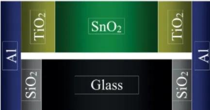
Figure 9.Measured type-B sensor impedanceZ(ZT, ZS,B, Za)in various atmospheres. All curves have been obtained with the same sensor specimen measured at various times. Case 1: N2with or without dry H2(orange and red solid lines, respectively). Case 2: N2with or without humid H2(light blue and dark blue dashed lines, respectively). Frequency from 10.3 Hz to 10 kHz.(a)Nyquist diagram and(b) Bode
diagram.
As revealed by Figs. 5 and 6 , the substrate (glass) conduc-tivity of a type-A sensor is about 100 times higher than that of the measurement environment at the same temperatures. Fig-ure 7 demonstrates that the type-B substrate (insulated glass) leads to a slightly higher shunt conductance (parallel to the coated IDT) than the test bed alone. This means that the test bed influence can be neglected for “high-conductivity” sub-strates as in type-A sensors, but must be taken into account with “low-conductivity” substrates as in type-B sensors.
Apart from this, the results clearly show that a layer thick-ness of about 200 nm (atomic force microscopy (AFM) mea-surements yielded a layer thickness, for the given sensor, of 175±5 nm) increases the resistivity of the substrate suffi-ciently.
To estimate the magnitude of the influence, we per-formed a numerical experiment based on measurement data for the test environment with a type-A substrate (yielding Z(ZT, ZS,A)), a type-B substrate (yielding Z(ZT, ZS,B)), and a type-B sensor (yielding Z(ZT, ZS,B, Za)) at 240◦C. The contributions of the active layerZa(f ), the substrate A ZS,A(f ), the substrate BZS,B(f ), and the test environment ZT(f )were calculated by solving Eq. (2). To simulate a test gas, the impedance of the active layerZa(f )was increased by 100 %, leading toZa,g(f )=2·Za(f ). The computations revealed that a sensor of type A would respond to this by an impedance increase of 3 % at low frequencies (10.3 Hz) and up to 92 % at high frequencies (10 kHz). In contrast, a type-B sensor would increase its impedance by 75 % at low frequen-cies (10.3 Hz) and 92 % at high frequenfrequen-cies (10 kHz). Type-C sensors would respond by even higher impedance increases. However, their low-conductivity substrate could not be mea-sured reliably. The type-C sensors are further discussed in Sect. 4.3.
As introduced in Fischerauer and Fischerauer (2011), the inflexion frequency in the Nyquist plot of the sensor impedance (cf. Fig. 5) strongly depends on temperature. Be-cause the dependency is non-linear, this could be used to de-termine the temperature of the sensor element (cf. Fig. 8).
The outliers in this plot are due to noise which perturbs the reconstruction algorithm for the inflexion frequency.
4.2 Influence of humidity
Figure 9 shows measurement results obtained for type-B sen-sors in various atmospheres (N2, with dry H2, with H2plus water). At first sight, one is inclined to think that the sen-sor resistance increases with humidity. In fact, however, hu-midity changes the sensor response to H2 only very little. The seeming humidity influence is due to the baseline drift inherent to the present sensors and resulting in time-variant impedance levels. We attribute the baseline drift to aging, re-laxation, poisoning or similar effects during the time interval between the measurements of cases 1 and 2 (about 6 h). Tem-perature fluctuations can be ruled out as source of the drift because they were held below 0.5◦C.
The assertation that humidity does not change the sensor response is corroborated by the fact that theshape of the Nyquist plot does not change with humidity and that charac-teristic quantities such as the sensor resistance, at say 10 Hz, vary with H2content, but not with humidity (said resistance decreases by 15 % when 10 % H2is added to the N2 atmo-sphere).
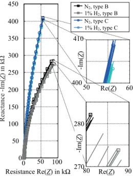
4.3 Influence of insulating substrates
To estimate the influence of the substrate, different sensors were characterized. Figure 10 shows the results for a B sensor (insulated glass substrate) as compared to a type-C sensor (quartz substrate). Although the impedance level of the former is lower by about 30 %, it still is in the same range as that of the latter. The variation visible in the figure is caused by noise, not by drift. No recognizable drift could be identified during the illustrated detail, because the repeatedly measured spectra did not “move” in a specific direction.
Resistance Re(Z) in kΩ
0 50 100
450
400
350
300
250
200
150
100
50
0
400
50 60
410
-Im(
Z
)
Re(Z)
80 90
280
270
-Im
(
Z
)
Re(Z) N2, type B 1% H2, type B N2, type C 1% H2, type C
Reactance -Im(
Z
) in kΩ
Figure 10.Measured impedances of a type-B sensor (squares) and a type-C sensor (circles). The dark symbols refer to measurement in pure N2repeated 7 times for each sensor type. The light symbols to measurement in N2plus 1 % H2(also repeated 7 times). Frequency
from 20 Hz to 10 kHz. Time interval between the repeated measure-ments was 2 min.
for the present purpose and a serious competitor of a supe-rior, but more expensive substrate such as quartz. Anyway, the impedance level of a type-B sensor, described by, e.g.,
Z(f =20 Hz), exceeds that of its type-A sensor counter-part by a factor of about 5.
Besides this, it can also be concluded from the curves in Fig. 10 that the response of the type-B and type-C sensors to hydrogen is similar. The respective reactances decrease by about 2 and 1 % in the two cases. We would not claim that type-B sensors systematically respond to H2more strongly than type-C sensors. Aging and other effects like fabrica-tion tolerances of the layer thicknesses could have a non-negligible impact on the sensor response.
We assume that the influence of the more conductive substrates (type-A) are caused by the ionic conductivity of the glass at elevated temperatures. For type-B sensors the amount of insulating SiO2suffice to disrupt this type of con-ductivity through the substrate. Quartz (type-C) is considered to be a nearly ideal insulator. We assume that the small dif-ferences between type-B and type-C substrates are caused by impurities in the insulating SiO2layer which enables a min-imum of ionic conductivity through the glass substrate.
5 Conclusion
We have demonstrated experimentally that the substrate plays an essential role for the overall performance of pla-nar H2sensors involving TiO2/SnO2thin films. Aspects of
the impedance spectrum (the inflexion frequency) of high-conductivity substrates (like glass, an ion conductor at el-evated temperatures) strongly depend on temperature and could therefore be used to recognize even small variations of the temperature.
Numerical experiments showed that high-conductivity substrates like glass can dominate the overall sensor response (impedance change) by 97 % at a frequency of 10.3 Hz. But a thin layer of SiO2 (200 nm) suffices to increase the impedance level. Thereby just about 25 % of the impedance increase is hidden by the substrate influence. Only sensors based on a highly insulating substrate like quartz can excel this.
Thin-film gas sensors do not need special properties of the substrate (like crystallinity) except the compatibility with thin-film technology and mechanical stability. Hence, there is no need to use expensive substrates such as quartz. By de-positing silicon dioxide on top of the substrate, even inex-pensive substrates like glass can be made to work.
Sensors with both conducting substrate plus insulating thin film and insulating substrate respond to H2 very similarly. Therefore, it can be excluded that the tested substrates in-fluence the sensing mechanism in an unacceptable manner. Furthermore, neither the test bed nor the sensors showed a cross-sensitivity to humidity.
Acknowledgements. The authors gratefully acknowledge support by the German Research Foundation (DFG) under contract number Fi 956/4-1.
Edited by: M. J. da Silva
Reviewed by: two anonymous referees
References
Barsan, N. and Weimar, U.: Conduction Model of Metal Oxide Gas Sensors, J. Electroceram., 7, 143–167, doi:10.1023/A:1014405811371, 2001.
Barsan, N., Koziej, D., and Weimar, U.: Metal oxide-based gas sen-sor research: How to?, Sensen-sor. Actuat. B-Chem., 121, 18–35, doi:10.1016/j.snb.2006.09.047, 2007.
Fischerauer, A. and Fischerauer, G.: Physikalisches Modell der Ma-terialparameterabhängigkeit des Impedanzspektrums planarer Chemosensoren in Mehrschichtbauweise, tm – Technisches Messen, 78, 15–22, doi:10.1524/teme.2011.0074, 2011. Fischerauer, A., Schwarzmüller, Ch., and Fischerauer, G.: Substrate
influence on the characteristics of interdigital-electrode gas sen-sors, Proc. Sixth Int’l Multi-Conf. on Systems, Signals & De-vices (SSD’09), Djerba, 5 pp., doi:10.1109/ssd.2009.4956738, 23–26 March, 2009.
Mardare, D., Iftime, N., and Luca, D.: TiO2 thin films as sensing gas materials, J. Non-Cryst. Solids, 354, 4396–4400, doi:10.1016/j.jnoncrysol.2008.06.058, 2008.
Simon, I., Bârsan, N., Bauer, M., and Weimar, U.: Micromachined metal oxide gas sensors: opportunities to improve sensor perfor-mance, Sensor. Actuat. B-Chem., 73, 1–26, doi:10.1016/S0925-4005(00)00639-0, 2001.