www.atmos-chem-phys.net/16/15119/2016/ doi:10.5194/acp-16-15119-2016
© Author(s) 2016. CC Attribution 3.0 License.
A high-resolution regional emission inventory of atmospheric
mercury and its comparison with multi-scale inventories:
a case study of Jiangsu, China
Hui Zhong1, Yu Zhao1,2, Marilena Muntean3, Lei Zhang4, and Jie Zhang2,5
1State Key Laboratory of Pollution Control & Resource Reuse and School of the Environment, Nanjing University, 163 Xianlin Ave., Nanjing, Jiangsu 210023, China
2Jiangsu Collaborative Innovation Center of Atmospheric Environment and Equipment Technology (CICAEET), Nanjing University of Information Science & Technology, Jiangsu 210044, China
3European Commission, Joint Research Centre, Institute for Environment and Sustainability, Air and Climate Unit, Via E. Fermi, Ispra, Italy
4University of Washington Bothell, 18115 Campus Way NE, Bothell, WA 98011, USA
5Jiangsu Provincial Academy of Environmental Science, 176 North Jiangdong Rd., Nanjing, Jiangsu 210036, China Correspondence to:Yu Zhao ([email protected])
Received: 20 June 2016 – Published in Atmos. Chem. Phys. Discuss.: 26 July 2016 Revised: 2 November 2016 – Accepted: 6 November 2016 – Published: 7 December 2016
Abstract. A better understanding of the discrepancies in multi-scale inventories could give an insight into their ap-proaches and limitations as well as provide indications for further improvements; international, national, and plant-by-plant data are primarily obtained to compile those invento-ries. In this study we develop a high-resolution inventory of Hg emissions at 0.05◦
×0.05◦
for Jiangsu, China, using a bottom-up approach and then compare the results with available global/national inventories. With detailed informa-tion on individual sources and the updated emission factors from field measurements applied, the annual Hg emissions of anthropogenic origin in Jiangsu in 2010 are estimated at 39 105 kg, of which 51, 47, and 2 % were Hg0, Hg2+
, and Hgp, respectively. This provincial inventory is thor-oughly compared to three downscaled national inventories (NJU, THU, and BNU) and two global ones (AMAP/UNEP and EDGARv4.tox2). Attributed to varied methods and data sources, clear information gaps exist in multi-scale inven-tories, leading to differences in the emission levels, speci-ation, and spatial distributions of atmospheric Hg. The to-tal emissions in the provincial inventory are 28, 7, 19, 22, and 70 % larger than NJU, THU, BNU, AMAP/UNEP, and EDGARv4.tox2, respectively. For major sectors, including power generation, cement, iron and steel, and other coal
com-bustion, the Hg contents (HgC) in coals/raw materials, abate-ment rates of air pollution control devices (APCDs) and ac-tivity levels are identified as the crucial parameters respon-sible for the differences in estimated emissions between in-ventories. Regarding speciated emissions, a larger fraction of Hg2+
is found in the provincial inventory than national and global inventories, resulting mainly from the results by the most recent domestic studies in which enhanced Hg2+
15120 H. Zhong et al.: A high-resolution regional emission inventory of atmospheric mercury 1 Introduction
Mercury (Hg), known as a global pollutant, has received in-creasing attention for its toxicity and long-range transport. Identified as the most significant release into the environ-ment (Pirrone and Mason, 2009; AMAP/UNEP, 2013), at-mospheric Hg is analytically defined as gaseous elemental Hg (GEM, Hg0), which has the longest lifetime and trans-port distance, and reactive gaseous mercury (RGM, Hg2+)
and particle-bound mercury (PBM, Hgp), which are more af-fected by local sources. Improved estimates in emissions of speciated atmospheric Hg are believed to be essential for bet-ter understanding the global transport, chemical behaviors, and mass balance of Hg.
Due mainly to the fast growth in economy and intensive use of fossil fuels, China has been indicated as the high-est ranking nation in anthropogenic Hg emissions (Fu et al., 2012; Pacyna et al., 2010; Pirrone et al., 2010). Emis-sions of speciated atmospheric Hg of anthropogenic origin in China have been estimated at both global and national scales. For example, AMAP/UNEP (2013) and Muntean et al. (2014) developed global Hg inventories which reported national emissions for China for 2010 and from 1970 to 2008, respectively. At the national scale, Hg emissions have been estimated based on more detailed provincial informa-tion on energy consumpinforma-tion and industrial producinforma-tion. Zhang et al. (2015), Zhao et al. (2015a), and Tian et al. (2015) eval-uated the inter-annual trends in emissions for 2000–2010, 2005–2012, and 1949–2012, respectively, to explore the ben-efits of air pollution control polices, particularly for recent years.
There are considerable information gaps between inven-tories, attributed mainly to the data of different sources and levels of details. For coal-fired power plants (CPP), as an ex-ample, the global inventories by AMAP/UNEP (2013) and Muntean et al. (2014) obtained the national coal consump-tion from the Internaconsump-tional Energy Agency (IEA), and they acquired the information on control technologies from the “national comments” by selected experts and World Electric Power Plants (WEPP) database, respectively. In the national inventories by Zhang et al. (2015) and Tian et al. (2015), coal consumption of CPP by province was derived from official energy statistics, and the penetrations of flue gas desulfuriza-tion (FGD) systems were assumed at provincial level. Zhao et al. (2015a) further analyzed the activity data and emission control levels plant by plant using a “unit-based” database of power sector. Although data of varied sources and levels of details result in discrepancies between inventories, those discrepancies and the underlying reasons have not been thor-oughly analyzed in previous studies, leading to large uncer-tainty in Hg emission estimation.
Existing global and national inventories could hardly pro-vide satisfying estimates in speciated Hg emissions or well capture the spatial distribution of emissions at regional/local scales, attributed mainly to relatively weak investigation of
individual sources. When they are used in a chemistry trans-port model (CTM), downscaled inventories at global/national scales would possibly bias the simulation at smaller scales. Improvement in emission estimation at local scale, partic-ularly for the large point sources, is thus crucial for better understanding the atmospheric processes of Hg (Lin et al., 2010; Wang et al., 2014; Zhu et al., 2015). While local in-formation based on sufficient surveys is proven to have ad-vantages in improving the emission estimates for given pol-lutants like NOxand PM10(Zhao et al., 2015b; Timmermans et al., 2013), there are currently very few studies on Hg emis-sions at regional/local scales in China, and the differences of multi-scale inventories remain unclear.
In this work, therefore, we select Jiangsu, one of the most developed provinces with serious air pollution in China, as study area. Firstly, we develop a high-resolution Hg emis-sion inventory of anthropogenic origin for 2010, based on a comprehensive review of field measurements and detailed information on emission sources. That provincial inventory is then compared to selected global and national inventories with a thorough analysis on data and methods. Discrepan-cies in emission levels, speciation, and spatial distributions are evaluated and the underlying sources of the discrepan-cies are figured out. Finally, the uncertainty in the provincial emission inventory is quantified and the key parameters con-tributing to the uncertainty are identified. The results provide an insight into the effects of varied approaches and data on development of the Hg emission inventory and indicate the limitations of current studies and the orientations for further improvement on emission estimation at regional/local scales.
2 Data and methods
2.1 Data sources of multi-scale inventories
As shown in Fig. S1 in the Supplement, Jiangsu province (30◦
45′
–35◦
20′
N, 116◦
18′
–121◦
57′
E) is located in the Yangtze River Delta in eastern China and covers 13 cities. The Hg emissions of Jiangsu are obtained from two ap-proaches: downscaled from global/national inventories and estimated using a bottom-up method with information on lo-cal sources incorporated.
In global/national inventories, Hg emissions were first cal-culated by sector based on activity data and emission fac-tors that were obtained or assumed at global, national, or provincial level, and were then downscaled to regional do-main with finer spatial resolution. Various methods and data were adopted in multi-scale inventories to estimate Hg emis-sions for different sectors, as summarized briefly in Table S1 in the Supplement. Three national inventories were devel-oped by Nanjing University (NJU; Zhao et al., 2015a), Bei-jing Normal University (BNU; Tian et al., 2015), and Ts-inghua University (THU; Zhang et al., 2015), with major activity data at provincial level obtained from Chinese
tional official statistics. Compared to the NJU and BNU in-ventories, which applied deterministic parameters relevant to emission factors, THU developed a model with proba-bilistic technology-based emission factors to calculate the emissions. Based on international activity statistics at na-tional level, two global inventories for 2010 were developed by the joint expert group of the Arctic Monitoring and As-sessment Programme and United Nations Environment Pro-gramme (AMAP/UNEP, 2013) and the Emission Database for Global Atmospheric Research (EDGARv4.tox2, unpub-lished). The AMAP/UNEP inventory developed a new sys-tem for estimating emissions from main sectors based on a mass-balance approach with data on unabated emission fac-tors and emission reduction technology employed in differ-ent countries. The EDGARv4.tox2 invdiffer-entory calculated the emissions for all the countries by primarily applying emis-sion factors from EEA (2009) and USEPA (2012), combined with regional technology-specific information on emission abatement measures.
2.2 Development of the provincial inventory
In contrast to the downscaling approach, the emissions are calculated plant by plant based on information on individual sources and then aggregated to provincial level in a bottom-up method. We refer to the inventory as the bottom-bottom-up or provincial inventory hereinafter. Information for individual emission sources are thoroughly obtained from the Pollution Source Census (PSC, internal data from the Environmental Protection Agency of Jiangsu Province). The PSC was con-ducted by local environmental protection agencies, in which the data for individual sources were collected and compiled through on-site investigation, including manufacturing tech-nology, production level, energy consumption, fuel quality, and emission control devices. Differences in total energy consumption and industrial production levels exist between the PSC data and the energy/economic statistics. For exam-ple, the coal consumption by power plants in the PSC was 6 % larger than the provincial statistics for Jiangsu in 2010. We believe that, compared to the energy and economic statis-tics that were commonly used in global/national invento-ries, the plant-by-plant PSC data could provide more detailed and accurate information on specific emitters, particularly for power and industrial plants.
According to the availability of data, anthropogenic sources are classified into three main categories. Category 1 includes coal-fired power plants (CPP), iron and steel plants (ISP), cement production (CEM), and other industrial coal combustion (OIB). Note that the emissions from coal com-bustion in cement production are not included in CEM but in OIB, following most other inventories included in this paper for easier comparison. The information on geo-graphic location, activity levels (consumption of energy or raw materials), and penetration of air pollution control de-vices (APCDs) is compiled plant by plant from the PSC,
with an exception that the technology employed in CEM is obtained from CCA (2011). Category 2 includes non-ferrous metal smelting (NMS), aluminum production (AP), municipal solid waste incineration (MSWI), and intentional use sector (IUS: thermometer, fluorescent lamp, battery, and polyvinyl chloride polymer production). Geographic loca-tion informaloca-tion for those sources is obtained from the PSC, while other activity data come from official statistics at provincial level. Category 3 includes emission sources that are not contained in the PSC: residential and commercial coal combustion (RCC), oil and gas combustion (O&G), biofuel use/biomass open burning (BIO), rural solid waste incinera-tion (RSWI), and human cremaincinera-tion (HC). They are defined as area sources, and the data sources for them are discussed later in this section.
In general, annual emissions of total and speciated Hg are calculated using Eqs. (1) and (2), respectively:
E=X n
ALn×EFn, (1)
Es =
X
n
ALn×EFn×Fn,s, (2)
whereE is the Hg emission, AL is the activity levels (fuel consumption or industrial production), EF is the combined emission factor (emissions per unit of activity level),F is the mass fraction of a given Hg speciation, andnandsrepresent emission source type and Hg speciation (Hg0, Hg2+
or Hgp). For CPP/OIB and CEM, Eq. (1) can be revised to Eqs. (3) and (4), respectively, with detailed fuel and technology infor-mation on individual sources incorporated:
ECPP/OIB=
X
t
X
i
X
k
ALi×HgCk×RRt×(1−REt) (3)
ECEM=
X
t
X
i
ALLimestone×HgCLimestone+ALOther,i ×HgCOther×(1−REt) , (4) where HgC is the Hg content of coal consumed in Jiangsu, calculated based on measured Hg contents of coal mines across the country and an inter-provincial flow model of coal transport (Zhang et al., 2015); HgCLimestone and HgCOther represent Hg contents of limestone and other raw materials (e.g., malmstone and iron powder) in cement production, re-spectively; RR is the Hg release ratios from combustors; RE is Hg removal efficiency of APCDs; ALLimestoneand ALOther represent the consumption of limestone and other raw mate-rials in CEM, respectively;iandkrepresent individual point source and coal type, respectively; andt represents APCD type, including wet scrubber (WET), cyclone (CYC), fab-ric filter (FF), electrostatic precipitator (ESP), FGD, and se-lective catalyst reduction (SCR) systems for CPP, as well as dry-process precalciner technology with dust recycling (DPT+DR), shaft kiln technology (SKT), and rotary kiln
15122 H. Zhong et al.: A high-resolution regional emission inventory of atmospheric mercury clinker and cement production when the information on
lime-stone or other raw materials is missing in the PSC. For ISP, Eq. (1) could be revised to Eq. (5):
EISP=
X
i
ALsteel,i+ALiron,i×R
×EFsteel, (5) where ALsteeland ALiron represent crude steel and pig iron production in ISP, respectively; R is the liquid steel to hot metal ratio provided by Remus et al. (2012), converting the production of pig iron to crude steel equivalent; and EFsteel is the Hg emission factor applied to steel making, obtained from recent domestic tests by Wang et al. (2016).
Activity data for NMS, AP, MSWI, RCC, and O&G are derived from national statistics (NMIA, 2011; NSB, 2011a, b), while Hg consumption in IUS is estimated based on the internal association commercial reports that provide na-tional market and economy information collected at http: //www.askci.com/. Activity data for MSWI, RSWI, and BIO are taken following Zhao et al. (2015a). Other information, including control efficiencies of APCDs, speciation profiles, and emission factors inherited from previous studies, is sum-marized in Tables S2–S4 in the Supplement.
Regarding the spatial pattern of emissions, the study do-main is divided into 4212 grid cells with a resolution at 0.05◦×
0.05◦
. For categories 1 and 2, emissions are directly allocated into corresponding grid cells according to the loca-tions of individual sources. As considerable errors in plant lo-cations were unexpectedly found in the PSC, the geographic locations for point sources with emissions more than 15 kg have been corrected by Google Maps. As a result, 900 plants in total are relocated, accounting for 14 % of all the point sources. For Category 3, emissions are allocated according to the population density in urban areas (RCC) and that in rural areas (BIO and RSWI).
2.3 Sensitivity and uncertainty analysis of emissions For better understanding the sources of discrepancies be-tween inventories, a comprehensive sensitivity analysis is conducted to quantify the differences between selected pa-rameters used in multi-scale inventories and the subsequent changes in emission estimation for Category 1 sources. The relative change (RC) in a given parameter (j) in global/national inventories compared to that in the provin-cial bottom-up inventory, as well as the changes in emissions for a selected source (n)when the value of parameterj in the bottom-up inventory is replaced by that in global/national in-ventories (Ediff,n), can be calculated using Eqs. (6) and (7),
respectively: RCj =
VOj−VBj
VBj
, (6)
Ediff,n=EOn−EBn, (7)
where VB is the value of parameters in the bottom-up inven-tory; VO is the value of parameters in other national/global
inventories; EB is Hg emissions for a given sector in the bottom-up inventory; EO is Hg emissions for a given sec-tor when the values of parameters in the bottom-up invensec-tory are replaced by those in other global/national inventories; and
j andnrepresent given parameter and source type, respec-tively.
In particular, a new parameter, total abatement rate (TA), is defined for the sensitivity analysis, combining the effect of the penetrations of APCDs and their removal efficiencies on emission abatement:
TA=X t
ARt×REt, (8)
wheretrepresents APCD type and AR and RE are the appli-cation rate and Hg removal efficiency, with detailed informa-tion provided in Table S5 in the Supplement.
The uncertainties in speciated Hg emissions at provincial level are quantified using a Monte Carlo framework (Zhao et al., 2011). Given the relatively accurate data reported in the PSC, the probability distributions of activity levels for individual plants of CPP, OIB, ISP, and CEM are defined as normal distributions with the relative standard deviations set at 10, 20, 20, and 20 % respectively. As summarized in Ta-bles S6 and S7 in the Supplement, a database for Hg emis-sion factors/related parameters by sector and speciation is established for China, with the uncertainties analyzed and indicated by probability distribution function (PDF). The PDFs of Hg contents in coal mines by province are ob-tained from Zhang et al. (2015). For Hg content in limestone (HgCLimestone), a lognormal distribution is generated with bootstrap simulation based on 17 field tests by Yang (2014), as shown in Fig. S2 in the Supplement. For the rest of the parameters, a comprehensive analysis of uncertainties was conducted, incorporating the data from available field mea-surements as described in Zhao et al. (2015a). Ten thousand simulations are performed to estimate the uncertainties in emissions, and the parameters that are most significant in de-termination of the uncertainties are identified by source type according to the rank of their contributions to variance.
3 Results and discussions
3.1 Emission estimation and comparison by sector 3.1.1 The total Hg emissions from multi-scale
inventories
Table 1 provides the Hg emissions by sector and species for Jiangsu in 2010 estimated from the bottom-up approach. The provincial total Hg emissions of anthropogenic origin are cal-culated to be 39 105 kg, of which 51 % is released as Hg0, 47 % as Hg2+
, and 2 % as Hgp. In general, categories 1, 2, and 3 account for 90, 4, and 6 % of the total emissions, re-spectively. CPP and CEM are the largest contributors to the
total Hg (HgT)emissions. For Hg0, Hg2+, and Hgp, the sec-tors with the largest emissions are CPP, CEM, and OIB re-spectively.
To better understand the discrepancies and their sources between various studies, the emissions from multi-scale in-ventories are summarized in Table 1 for comparison. Among all the inventories, the total emissions in the provincial in-ventory are the largest, i.e., 28, 7, 19, 22, and 70 % higher than NJU, THU, BNU, AMAP/UNEP, and EDGARv4.tox2, respectively. The elevated Hg emissions compared to previ-ous studies could be supported by modeling and observation work to some extent. Based on the chemistry transport mod-eling using GEOS-Chem (Wang et al., 2014), or correlation slopes with certain tracers (CO, CO2, and CH4)from ground observation (Fu et al., 2015), underestimation was suggested for the regional Hg emissions of anthropogenic origin in China.
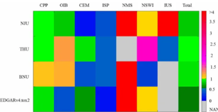
Direct comparison between inventories is unavailable for every sector, as the definition of source categories is not fully consistent with each other. Therefore, necessary as-sumption and modification are made on source classifica-tion for global inventories. In Table 1, CPP, OIB, and RCC for EDGARv4.tox2 represent the emissions for all of the fossil fuel types, and they are 1316 and 5342 kg lower and 986 kg higher than our estimation from coal combustion, re-spectively. For AMAP/UNEP, the emissions from regrouped stationary combustion (industrial sources excluded), indus-try, and intentional use and product-waste-associated sources (see Table 1 for the detailed definition) are respectively 3382 and 2032 kg higher and 3118 kg lower than our estimation with the bottom-up method. Figure 1 shows the ratios of the estimated Hg emissions in national/global inventories to those in the provincial inventory by source. The CPP emis-sions are relatively close to each other, but larger differences exist in some other sources. The estimates for CEM and ISP in the provincial inventory are much higher than the NJU, BNU, and EDGARv4.tox2 inventories, while those for NMS are considerably smaller. The reasons for those differences are analyzed in detail in Sect. 3.1.2–3.1.4.
3.1.2 Sensitivity analysis for power plants and industrial boilers
Figure 2a and b represent the relative changes in given pa-rameters between the provincial and other inventories, and the subsequent differences in Hg emissions for Category 1 sources, using Eqs. (6) and (7), respectively. For CPP, the dif-ferences between provincial and national/global inventories are mainly determined by AL, HgC, TA, and IEF (integrated emission factors), as indicated by the calculation methods summarized in Table S1. (Instead of analyzing HgC and RR separately, integrated input emission factors were applied in AMAP/UNEP and EDGARv4.tox2.) For activity level (AL), the coal consumption data are collected and compiled plant by plant in the provincial inventory, while they were obtained
Figure 1. The ratios of estimated Hg emissions for Jiangsu and 2010 in global/national inventories to that in the provincial inven-tory for selected sources and anthropogenic total.
‐1.2 ‐0.7 ‐0.2 0.3 0.8 1.3 Hg Cr a
w AL TA IEF
Hg
Cr
a
w AL TA RR AL TA UEF AL
EF ir on E F st eel
CPP OIB CEM ISP
(a)
NJU THU BNU AMAP/UNEP EDGARv4.tox2
Relati v e ch ang e s
‐11 000
‐9000 ‐7000 ‐5000 ‐3000 ‐1000 1000 3000 Hg Cr a
w AL TA IEF
Hg
Cr
a
w AL TA RR AL TA UEF AL
EF ir on E F st eel
CPP OIB CEM ISP
(b)
NJU THU BNU AMAP/UNEP EDGARv4.tox2
Diff eren ce s in Hg emis si o n s (kg )
Figure 2.Sensitivity analysis of selected parameters in Hg emission estimation for Category 1 sources.(a)Relative changes in param-eters, calculated using Eq. (6), and(b)changes in emissions when parameters in the provincial inventory were replaced with those in other inventories, calculated using Eq. (7). HgCraw: Hg content in raw coal; AL: activity levels as raw coal consumption by CPP and OIB, limestone used by CEM, and crude steel produced in ISPs; TA: total abatement rate of APCDs; RR: Hg release rate for combus-tion; IEF: input emission factors (before control of APCDs); UEF: uniform emission factor (without consideration of different APCD types); EFiron and EFsteel: emission factors of pig iron and steel production, respectively.
15124
H.
Zhong
et
al.:
A
high-r
esolution
regional
emission
in
v
entory
of
atmospheric
mer
cury
Table 1.Emission estimates for Jiangsu in 2010 and species from multi-scale inventories by sector. Abbreviations for emission sources, as in Sect. 2 – CPP: coal-fired power plants; RCC: residential coal combustion; O&G: oil and gas combustion; OIB: other industrial coal combustion; CEM: cement production; ISP: iron and steel plants; NMS: nonferrous metal smelting; AP: aluminum production; LGM: large-scale gold mining; MM: mercury mining; HC: human cremation; MSWI: municipal solid waste incineration; RSWI: rural solid waste incineration; BFLP: battery/fluorescent lamp production; BIO: biofuel use/biomass open burning; and PVC: PVC production.
CPP1 RCC3 O&G3 OIB1 CEM1 ISP1 NMS2 AP2 LGM MM HC3 MSWI2 RSWI3 BFLP2 BIO3 PVC2 Total
HgT Bottom-up 11 549 195 930 8652 9264 5654 91 29 0 0 326 1009 365 158 461 423 39 106 NJU 11 208 165 930 6901 1137 2243 2158 – 23 51 – 1009 457 1225 500 2603 30 610 THU 10 768 345 752 10 680 8238 2539 0 29 0 0 326 2294 244 219 – 36 434 BNU 12 883 267 898 10 172 3288 2669 2022 6 – – – 308 303 – 32 816 AMAP/UNEP 9292a 17 759b 4976c – – 32 027 EDGARv4.tox2 10 233d 1181e – 3310f 6364 447 413 – – – – 1017 – 43 – 23 008
Hg0 Bottom-up 8811 91 465 4689 2461 1908 45 23 0 0 313 131 47 158 350 423 19 915 NJU 8133 42 465 2042 685 1208 1189 – 16 41 – 190 393 980 380 2082 17 846 THU 7689 247 376 6995 2793 863 0 23 0 0 313 2202 244 162 – 21 907 AMAP/UNEP 4646a 14 207b 4668c – – 23 521
Hg2+
Bottom-up 2653 73 372 3394 6752 3746 45 4 0 0 0 868 314 0 23 0 18 244 NJU 2900 45 372 4003 431 835 963 – 7 8 – 868 59 184 25 390 11 090 THU 3058 92 301 3471 5338 1676 0 4 0 0 0 0 0 11 – 13 951 AMAP/UNEP 3717a 2707b 238c – – 6662
Hgp Bottom-up 85 32 93 569 51 0 0 1 0 0 13 10 4 0 88 0 946 NJU 175 79 93 855 20 200 6 – 0 3 – 10 5 61 95 130 1732 THU 22 6 75 214 107 0 0 1 0 0 13 92 0 46 – 576 AMAP/UNEP 929a 845b 70c – – 1844
1,2,3Sectors in Category 1, 2, and 3 as classified in Sect. 2.aStationary combustion sources: power plants, distributed heating, and other energy use (industrial sources excluded).bIndustrial sources including stationary combustion for
industry, CEM, ISP, NMS, AP, LGM, and MM.cIntentional use and product-waste-associated sources: artisanal and small-scale gold mining, solid waste incineration and other product waste disposal, chlor-alkali industry, and human cremations.d,e,fBoth coal and other fossil fuel combustion included.
Atmos.
Chem.
Ph
ys.,
16,
15119–
15134
,
2016
www
.atmos-chem-ph
In national and provincial inventories, as mentioned in Sect. 2, the Hg contents in the raw coal (HgCraw)consumed by province are estimated using an inter-provincial flow ma-trix for coal transport based on the results of field measure-ments on Hg contents for given coal mines (Tian et al., 2010, 2014; Zhang et al., 2012). The HgCrawfor Jiangsu in THU and our provincial inventory come from Zhang et al. (2012), who merged the results of two comprehensive measurement studies on HgCraw(by themselves and USGS, 2004) for coal mines across China after 2000, and the average value is calculated at 0.2 g t−1coal. The NJU inventory adopted the HgCrawof 0.169 g t−1coal from Tian et al. (2010), while the BNU inventory determined HgCrawat 0.25 g t−1coal with a bootstrap simulation based on a thorough investigation of published data (Tian et al., 2014). HgCraw in the NJU and BNU inventories are 15 % smaller and 25 % higher than that in the provincial inventory, leading to differences of 1746 and 2816 kg in Hg emissions, respectively. Given the large differences in HgCrawbetween countries, global inventories applied national specific IEFs based on the domestic tests (UNEP, 2011b; Wang et al., 2010). The IEFs for China ap-plied in AMAP/UNEP and EDGARv4.tox2, without consid-ering the regional differences in HgCraw, are 26 and 28 % lower than that in the provincial inventory (recalculated with HgCrawand RR). As regional HgCrawdiffers a lot from the national average and could be largely influenced by the data selected, a large discrepancy might exist when the national value is applied in the regional inventory, and more regional-specific measurements are suggested for reducing the uncer-tainty.
Total abatement rate (TA) of APCDs installed for CPP is calculated at 57 % in the provincial inventory, 6.7 and 8.2 % smaller than that in the THU and AMAP/UNEP in-ventories, respectively, and 12 % larger than that in the NJU inventory. The differences result mainly from the varied removal efficiencies (RE) and application ratios (AR), as shown in Table S5. For RE, local tests on FF, ESP+FGD, and SCR+ESP+FGD were conducted by JSEMC (2013)
and Xie and Yin (2014), and the results (provided in Ta-ble S2) are applied in the provincial inventory. From in-vestigation of individual plants, the AR of FGD systems with relatively large benefits on Hg removal was underes-timated in NJU and overesunderes-timated in the THU inventory. In the AMAP/UNEP inventory, relevant parameters were ob-tained from national comment, and elevated TA was esti-mated due to the larger AR of FF and FGD and the higher RE of FGD+ESP compared to that obtained from detailed source investigation in the provincial inventory.
For OIB, the comparison of HgC is similar to that for CPP. AL from the PSC in the provincial inventory is very close to that in the THU inventory obtained from NSB (2011b), while AL in the NJU inventory was much lower as the coal consumption of CEM and ISP was excluded. The RR from industrial boilers in this work is estimated at 82 % based on domestic measurements (Wang et al., 2000; Tang et al.,
2004), much lower than the result in the THU inventory mea-sured by Zhang et al. (2012), i.e., 95 % for stoker-fired boil-ers. Given the limited samples in both inventories, large un-certainty exists in RR of industrial boilers. Compared to the provincial inventory, ARs of ESP and FGD were clearly un-derestimated in the NJU and THU inventories (Table S5); hence, the TA in NJU was calculated 23 % smaller than that in the provincial inventory, leading to a 747 kg increase in the Hg emission estimate. In the THU inventory, however, the much higher RE of WET reduced the difference between national and provincial inventories, and TA in the THU in-ventory was only 2 % smaller than the provincial one.
3.1.3 Sensitivity analysis for cement and iron and steel industries
For CEM, both the provincial and THU inventories adopted the data from Yang (2014), who measured provincial Hg con-tents in raw materials (limestone and other raw materials) and Hg removal efficiency of DPT+DR in China. For AL, the limestone consumption were calculated based on the clinker and cement production of individual plants in the provincial inventory, while THU relied on cement production at provin-cial level, leading to 13 % smaller in AL and 1019 kg reduc-tion in the Hg emission estimate. In addireduc-tion, consumpreduc-tion of other raw materials for CEM was ignored in the THU inven-tory, leading to 1223 kg smaller in emission estimate com-pared to the provincial inventory. According to an on-site sur-vey by Yang (2014), fly ash is 100 % reused in DPT+DR, and thus the technology minimizes the Hg removal by dust collectors (ESP or FF). The AR of DPT+DR in THU was estimated at 82 % at national average level, while it reaches 89 % in Jiangsu based on detailed provincial statistics (CCA, 2011). Hence, the TA employed in THU is 25 % larger than that in the provincial inventory, resulting in 259 kg underes-timation in Hg emissions. The NJU and AMAP/UNEP in-ventories failed to characterize the poor control of Hg from DPT+DR. EFs applied in NJU came from early
domes-tic measurements on rotary and shaft kiln (Li, 2011; Zhang, 2007), ignoring the recent penetration of DPT+DR. In the
AMAP/UNEP inventory, an effective Hg capture of 40 % was generally assumed for China’s cement plants, taking only the use of ESP and FF into account. The TA was estimated 215 % larger than that in the provincial inventory, resulting in a 2253 kg reduction in the Hg emission estimate. EDGAR applied uniform emission factor (UEF) of 0.065 g t−1clinker from EEA (2009), 32 % lower than the average EF in the provincial inventory. BNU developed S-shaped curves to es-timate the time-varying dynamic emission factors for non-coal combustion sector, based on the assumption of a grad-ually declining trend in EFs along with increased controls of APCDs. As mentioned above, however, the trend was not suitable for CEM due to the penetration of DPT+DR. Thus,
15126 H. Zhong et al.: A high-resolution regional emission inventory of atmospheric mercury underestimation in Hg emissions, e.g., 7261 kg smaller than
our provincial inventory.
For ISP, difficulty exists in emission estimation due to var-ious Hg input sources and complex production processes, and there is no consistent method in multi-scale invento-ries so far. It was found that raw material production (lime-stone and dolomite), coking, sintering, and pig iron smelting with blast furnace account for most Hg emissions in typi-cal ISPs in China (Wang et al., 2016). In our study, 11 fac-tories containing those processes are collected in the PSC, and the emissions factors of 0.043 and 0.068 g t−1crude steel from Wang et al. (2016) are applied to plants with and with-out raw material production, respectively. In other inven-tories, very few results from domestic measurements were applied for Hg emission estimation for ISP in China. NJU took only coal combustion into account and thus underesti-mated the emissions for the sector by neglecting the Hg in-put along with iron ore, limestone and other raw materials. THU applied an emission factor of 0.04 g t−1 from Pacyna et al. (2010) for crude steel production. Besides differences in emission factors, THU did not count the pig iron produc-tion in AL estimaproduc-tion, and thus AL in the THU inventory is 29 % lower than that in the provincial inventory, result-ing in 1615 kg reduction in the Hg emission estimate. Av-erage EF in AMAP/UNEP was estimated at 0.039 g t−1pig iron by combining the input factor (0.05 g t−1pig iron) cal-culated with a mass-balance method (UNEP, 2011a; Remus et al., 2012), and the removal effects of APCDs. For compar-ison, EF used in our provincial inventory was recalculated at 0.064 g t−1pig iron based on the hot metal charging ratio (R in Eq. 5; Remus et al., 2012). Lower EF in AMAP/UNEP can partly be attributed to the overestimated AR of APCDs in ISP without considering the gradual penetration of dust recycling as in CEM.
In general, the detailed activity and technology informa-tion including manufacturing procedures and APCDs was in-vestigated for individual plants in our provincial inventory to improve the emission estimation, in contrast to previous inventories that applied simplified or regional-average data. However, some crucial parameters (e.g., Hg contents in coal and limestone, and Hg removal efficiencies of APCDs) are still unavailable at plant level due to a lack of measurements. Such a limitation indicates the necessity of more efforts on plant-specific emission factors and also motivates the uncer-tainty analysis for the provincial inventory, as presented in Sect. 3.4.
3.1.4 Comparisons of emissions for categories 2 and 3 For categories 2 and 3, differences also exist in EF and AL between inventories. For example, an emission factor of 0.22 g t−1waste combusted for MSWI based on domes-tic tests (L. Chen et al., 2013; Hu et al., 2012) is applied in the provincial inventory, while THU applied 0.5 g t−1 from UNEP (2011a), resulting in a difference of 1024 kg in
emis-sion estimate. For primary Cu production, the provincial in-ventory applied the emission factor of 0.4 g t−1Cu from Wu et al. (2012), who incorporated the results of available field measurements and the penetrations of different smelting pro-cesses in China. BNU, however, applied a much higher emis-sion factor at 8.9 g t−1Cu estimated by using an S-shaped curve based on international results (Habashi, 1978; Nriagu, 1979; Pacyna, 1984; Pacyna and Pacyna, 2001; Streets et al., 2011; EEA, 2013). In the NJU inventory, the emis-sions from NMS and IUS were estimated much higher than the provincial inventory, attributed largely to the different sources of activity data. For NMS, activity levels in the NJU and provincial inventories were obtained from NSB (2011c) and NMIA (2011), respectively. While NMIA (2011) pro-vides the information on the production of primary nonfer-rous metal (the major source of Hg emissions for NMS), the secondary production was included in NSB (2011c), lead-ing to a possible overestimate in AL and thus Hg emissions. For IUS, provincial Hg consumption was allocated from the national total use weighted by GDP in the NJU inventory, while the data are directly derived for Jiangsu from internal industrial report in the provincial inventory. In the global in-ventories, moreover, all the emissions for categories 2 and 3 in Jiangsu were downscaled from national estimations at-tributed to a lack of provincial information, and large bias could be expected. For example, the large discrepancy for in-tentional use and product-waste-associated sources between downscaled global and provincial inventories is likely at-tributed to the overestimation in emissions from artisanal and small-scale gold mining (ASGM) by global inventory (not included in Table 1 as no ASGM was found by local source investigation).
3.2 Hg speciation analysis of multi-scale inventories Besides the total emissions, Hg speciation has a significant impact on the distance of Hg transport and chemical behav-iors. Table 2 summarizes the mass fractions of Hg species in emissions by sector for multi-scale inventories.
In general, as shown in Table 2, reduced Hg0, but en-hanced Hg2+
, is estimated as the spatial scale gets smaller. This can be mainly explained by the use of domestic mea-surement results on Hg speciation for CEM, ISP, and MSWI in the provincial inventory. For CEM, the Hg2+
mass frac-tion for the dominant DPT+DR technology tends to reach 75 % based on available measurements (Yang, 2014), leading to a much larger fraction of Hg2+emissions in the
provin-cial inventory. In contrast, speciated Hg emissions were cal-culated using the same speciation profiles as those for coal combustion in the NJU inventory or the uniform profile ig-noring the effects of APCDs in the AMAP/UNEP inventory. For ISP, heterogeneous Hg oxidation can be enhanced by the high concentration of dust and existence of Fe2O3in the flue gas during sintering process, leading to large Hg2+
fraction for the sector reaching 66 % (Wang et al., 2016). For MSWI,
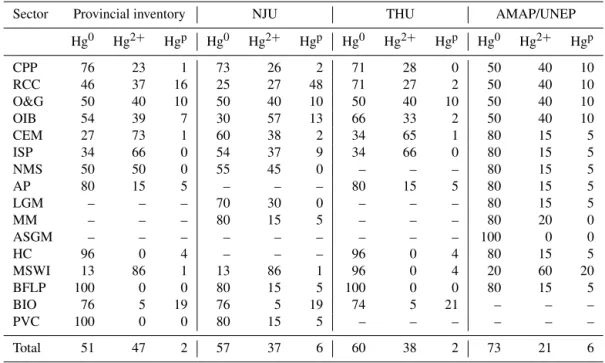
Table 2.Hg speciation profiles by sector and the mass fractions to total emissions in multi-scale inventories (%).
Sector Provincial inventory NJU THU AMAP/UNEP
Hg0 Hg2+ Hgp Hg0 Hg2+ Hgp Hg0 Hg2+ Hgp Hg0 Hg2+ Hgp
CPP 76 23 1 73 26 2 71 28 0 50 40 10
RCC 46 37 16 25 27 48 71 27 2 50 40 10 O&G 50 40 10 50 40 10 50 40 10 50 40 10 OIB 54 39 7 30 57 13 66 33 2 50 40 10
CEM 27 73 1 60 38 2 34 65 1 80 15 5
ISP 34 66 0 54 37 9 34 66 0 80 15 5
NMS 50 50 0 55 45 0 – – – 80 15 5
AP 80 15 5 – – – 80 15 5 80 15 5
LGM – – – 70 30 0 – – – 80 15 5
MM – – – 80 15 5 – – – 80 20 0
ASGM – – – – – – – – – 100 0 0
HC 96 0 4 – – – 96 0 4 80 15 5
MSWI 13 86 1 13 86 1 96 0 4 20 60 20
BFLP 100 0 0 80 15 5 100 0 0 80 15 5
BIO 76 5 19 76 5 19 74 5 21 – – –
PVC 100 0 0 80 15 5 – – – – – –
Total 51 47 2 57 37 6 60 38 2 73 21 6
results of domestic measurements (L. Chen et al., 2013; Hu et al., 2012) were applied in the provincial and NJU inven-tories, elevating the Hg2+
fraction compared to THU and AMAP/UNEP inventories that applied a global uniform spe-ciation profile without consideration of regional difference. It should be noted, however, that uncertainty exists in the estimation of speciated emissions at small spatial scale, at-tributed mainly to the limited samples in domestic measure-ments on CEM and ISP.
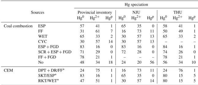
As mentioned above, the “universal” profiles were applied for many sectors in the AMAP/UNEP inventory, ignoring the effects of various types of APCDs on Hg speciation, particu-larly for coal combustion. However, the fate of Hg released to atmosphere can primarily be affected by the removal mech-anisms of APCDs. As shown in Table 3, for example, Hg0 mass fractions for ESP+FGD and FF+FGD tend to be
high, reaching 83 and 78 %, respectively, attributed to the relatively strong removal effects of APCDs on Hg2+
and Hgp. Once SCR is applied, an increase in the Hg2+
fraction can be observed, as the catalyst in SCR system can accel-erate the conversion of Hg0 to Hg2+ (Wang et al., 2010).
In addition, Hg0 can also be oxidized to Hg2+ in FF
at-tributed to specific chemical composition in flue gas (chlo-rine, for example) and to high temperature (Wang et al., 2008; He et al., 2012). Therefore, in contrast to global in-ventories, national and provincial inventories take the effects of different APCDs into account. Summarized in Table 3, considerable differences exist in the speciation profiles for typical APCDs between national and provincial inventories, attributed mainly to the various data used from domestic field measurements. Excluding the measurement results on
WET (Zhang et al., 2012), NJU assumed same species pro-file for WET and CYC, and thereby largely underestimated the mass fraction of Hg0 for OIB, where WET is widely applied. Furthermore, the penetrations of APCDs are also crucial in determination of speciated Hg emissions. As in-dicated in Table 3, with similar speciation profiles for FGD applied between multi-scale inventories, the difference in Hg speciation is relatively small for CPP between inventories, given the relatively accurate and transparent information on FGD penetration in CPP. For OIB, however, the difference in Hg speciation is significantly elevated, as large diversity in APCDs penetration is found between multi-scale invento-ries, as shown in Table S5. With the penetration of FF and ESP highly underestimated, for example, THU provided a lower estimation in Hg2+
fraction compared to other inven-tories.
3.3 Comparisons of spatial patterns of emissions between multi-scale inventories
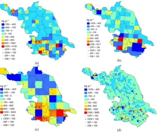
Figure 3 presents the spatial distributions of total and spe-ciated Hg emissions in Jiangsu province at 0.05◦×0.05◦
dom-15128 H. Zhong et al.: A high-resolution regional emission inventory of atmospheric mercury
Table 3.Hg speciation profiles used in provincial and national inventories for typical APCDs (%).
Hg speciation
Sources Provincial inventory NJU THU Hg0 Hg2+ Hgp Hg0 Hg2+ Hgp Hg0 Hg2+ Hgp
Coal combustion ESP 57 41 1 65 35 0 58 41 1
FF 31 61 7 16 73 11 50 49 1
WET 65 33 2 30 57 13 65 33 2
CYC 30 57 14 30 57 13 – – –
ESP+FGD 83 16 0 83 16 0 84 16 1 SCR+ESP+FGD 71 29 0 72 28 0 74 26 0
FF+FGD 78 21 1 – – – 78 21 1
No 48 34 18 24 20 56 56 34 10
CEM DPT+DR/FF∗ 24 75 1 16 73 11 24 76 1 SKT/ESP∗ 83 16 1 65 35 0 80 15 5
RKT/WET∗ 47 51 1 30 57 14 80 15 5
∗DPT+DR, SKT, and RKT are for the provincial and THU inventory (Zhang et al., 2015); FF, ESP, and WET are for the NJU inventory (Zhao et al.,
2015a).
Figure 3.Spatial distribution of Hg emissions for Jiangsu 2010 at a resolution of 0.05◦×0.05◦for(a)HgT,(b)Hg0,(c)Hg2+, and(d)Hgp.
inate the Hg emissions compared to the subsequent mixing stage (UNEP, 2011a) are mainly located in southern Jiangsu, depending on the distribution of limestone resources.
In order to compare the spatial distribution of the provin-cial inventory to that of the NJU, THU, AMAP/UNEP,
and EDGARv4.tox2 inventories, we upscale the gridded provincial emissions from 0.05◦×
0.05◦
to the resolutions of 0.125◦×
0.125◦
, 36×36 km, 0.5◦×0.5◦, and 0.1◦×0.1◦
respectively. Differences in gridded HgT emissions for Jiangsu between the upscaled provincial inventory and
Figure 4. Differences in gridded HgTemissions in Jiangsu 2010 between provincial and other inventories: emissions in the provincial inventory minus those in NJU(a), THU(b), AMAP/UNEP(c), and EDGARv4.tox2(d). The locations of point sources with relatively large Hg emissions estimated in the provincial inventory are indicated in the panels as well.
other multi-scale inventories are presented in Fig. 4. Al-though selected sources were identified as point sources in global/national inventories, e.g., CEM in NJU and THU, ISP in EDGARv4.tox2, and CPP in all the inventories, the emis-sion fraction of point sources (categories 1 and 2) is signif-icantly elevated to 92 % in the provincial inventory. In par-ticular, the emissions from point sources of which the geo-graphic information were corrected account for 78 % of total emissions in the province.
As illustrated in Fig. 4, differences in gridded emis-sions between provincial and other inventories (NJU, THU, AMAP/UNEP, and EDGARv4.tox2) are respectively in the ranges of −760 to +4135, −1429 to +3217, −1424 to +3043 and −1078 to +3895 kg. Grids with differences more than 400 kg yr−1 are commonly distributed in south-ern and northwestsouth-ern Jiangsu, and coincide well with the locations of point sources with relatively large emissions in the provincial inventory. It can be indicated that differ-ences in spatial patterns of Hg emissions come mainly from the inconsistent information on large point sources between the provincial inventory and national/global inventories. For CPP, AMAP/UNEP obtained information on identified facil-ities from Wikipedia (http://en.wikipedia.org/wiki/List_of_ power_stations_in_Asia) and failed to include a number of CPPs built in recent years (Steenhuisen and Wilson, 2015).
15130 H. Zhong et al.: A high-resolution regional emission inventory of atmospheric mercury The comparison in northwestern Jiangsu is less conclusive:
the emissions in the areas with large power plants were esti-mated lower in the provincial inventory than AMAP/UNEP (Fig. 4c). Such a difference, however, results not only from the varied estimations in CPP emissions but also from dis-crepancy in other sources, e.g., intensive emissions from in-dustrial sources in the area in AMAP/UNEP. For ISP and CEM, similarly, higher emissions were estimated by the provincial inventory for areas with large plants in Zhenjiang, Suzhou, and Changzhou in southern Jiangsu. In contrast to the provincial inventory that investigated the activities of each manufacturing processes for individual plants, the emis-sions in national inventories (THU and NJU) were allocated based only on the production of plants, ignoring the effects of manufacturing technologies on emissions. Moreover, some CEM and ISPs were missed in those national inventories, leading to underestimation in emissions for corresponding regions. When the national inventory was applied in CTM, the simulated concentrations of HgTwere usually lower than the observation at rural sites in eastern China (Wang et al., 2014). Since many large plants are being moved from urban to rural areas (Zhao et al., 2015b; Zhou et al., 2016), im-provement in model performance could be expected when the elevated emissions in rural areas are estimated and used for CTM, incorporating the accurate information on individ-ual large plants.
With much fewer large emitters, discrepancies in grid-ded emissions for another part of Jiangsu resulted largely from the allocation of emissions as area sources in national and global inventories. For example, in spite of an estima-tion of 8496 kg smaller than the provincial inventory in total emissions, the NJU inventory applied proxies (e.g., popula-tion and GDP) to allocate the emissions except those from CPP, resulting in higher emissions in central and most part of northern Jiangsu (Fig. 4). Similar patterns are also found for THU (Fig. 4b) and AMAP/UNEP (Fig. 4c) compared to the provincial inventory.
Besides the total emissions, differences in spatial distri-bution of speciated Hg emissions between multi-scale in-ventories are presented in Fig. S3 in the Supplement. The various patterns for species are largely influenced by the distribution of different types of large point sources, as the speciation profiles vary significantly between source types in the national and provincial inventories (Table 2). Com-pared to other inventories, larger Hg0emissions were found in the provincial inventory in southern Jiangsu (particularly Zhenjiang and Taizhou), where CPPs with a large fraction of Hg0are heavily concentrated. Elevated Hg2+
emissions were dominated by intensive CEM industry in Changzhou, Wuxi, and Zhenjiang in southern Jiangsu, as the Hg2+
fraction of CEM reaches 73 % in the provincial inventory. Differences in Hgpemissions between inventories in central Jiangsu are closely related to the locations of OIB plants, attributed mainly to the relatively poor understanding of the particle control and thereby Hgp release of OIB. The emissions in
the provincial inventory are larger than THU but smaller than AMAP/UNEP, as the Hgpmass fraction of OIB was assumed at 2 % in THU, while it reached 10 % in AMAP/UNEP (Ta-ble 2).
The vertical distribution of Hg releases, which is crucial for the transport range of atmospheric Hg, is also analyzed. Four groups of release height are defined: 0–58, 58–141, 141–250, and > 250 m. Based on the detailed information on emission sources, the fractions of Hg releases into the four groups for CPP are 2, 66, 31, and 1 %, respectively, and the analogue numbers for OIB, ISP, and CEM are 85, 13, 2, and 0; 4, 44, 12, and 4 %; and 6, 94, 0, and 0 %, respectively. The release heights for rest sources are uniformly assumed to be in the range of 0–58 m. As a result, the fractions of to-tal Hg emissions in the four groups are estimated as 35, 53, 11, and 1 %. In the AMAP/UNEP inventory, as a compari-son, the fractions at the height of 0–50, 50–150, and > 150 m were estimated at 23, 53, and 24 % respectively, with a larger share in Hg emitted over 150 m than that in our provincial inventory. The smaller fraction of Hg emissions under 150 m and larger fraction of Hg2+
as discussed in Sect. 3.2 in the provincial inventory are expected to result in more local de-position and less long-range transport compared to previ-ous inventories when they are applied in the CTM. The re-emissions of legacy Hg could then be enhanced and make a significant contribution to atmospheric Hg concentrations, as indicated by Zhu et al. (2012).
3.4 Uncertainty in the provincial inventory
As summarized in Table 4, the uncertainties in speciated Hg emissions in the provincial inventory are estimated at−24 to
+82 % (95 % confidence intervals around central estimates),
−34 to+99,−23 to 68, and−34 to+270 % for HgT, Hg0, Hg2+
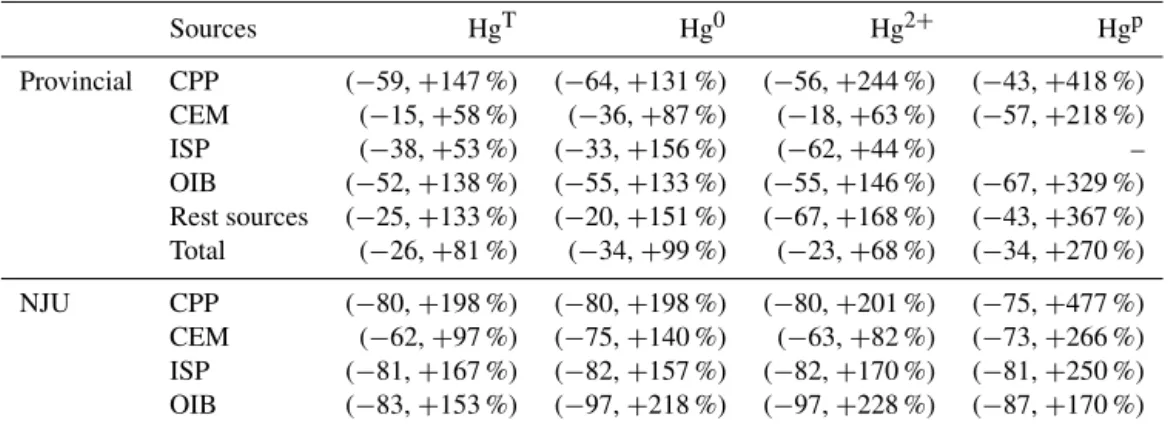
, and Hgp, respectively. For comparison, the uncertain-ties in Jiangsu emissions from major sectors including CPP, CEM, ISP, and OIB in NJU inventory are recalculated fol-lowing Zhao et al. (2015a) and provided in Table 4 as well. The uncertainties for major sources in the provincial inven-tory were smaller than those in the NJU inveninven-tory, attributed largely to the bottom-up approach used in the provincial in-ventory with more accurate information on activity levels and APCDs applications for individual plants of Category 1. In addition, with more field measurements of Hg contents in coal and limestone incorporated, the uncertainties in HgCraw and HgCLimestone are significantly reduced, resulting from the mechanism of error compensation when HgCrawof coals produced in different provinces is taken into account in the inter-provincial flow model for coal transport and from the success in bootstrap simulation, respectively. As a result, the uncertainties in emissions from CPP, OIB, and CEM are ef-fectively reduced in the provincial inventory.
The parameters contributing most to uncertainties and their contributions to the variance of corresponding emission estimates are summarized by sector in Table S8 in the
Table 4.Uncertainties in Hg emissions in Jiangsu in provincial and national (NJU) inventories by source, expressed as the 95 % confidence intervals of central estimates.
Sources HgT Hg0 Hg2+ Hgp
Provincial CPP (−59,+147 %) (−64,+131 %) (−56,+244 %) (−43,+418 %) CEM (−15,+58 %) (−36,+87 %) (−18,+63 %) (−57,+218 %) ISP (−38,+53 %) (−33,+156 %) (−62,+44 %) – OIB (−52,+138 %) (−55,+133 %) (−55,+146 %) (−67,+329 %) Rest sources (−25,+133 %) (−20,+151 %) (−67,+168 %) (−43,+367 %) Total (−26,+81 %) (−34,+99 %) (−23,+68 %) (−34,+270 %)
NJU CPP (−80,+198 %) (−80,+198 %) (−80,+201 %) (−75,+477 %) CEM (−62,+97 %) (−75,+140 %) (−63,+82 %) (−73,+266 %) ISP (−81,+167 %) (−82,+157 %) (−82,+170 %) (−81,+250 %) OIB (−83,+153 %) (−97,+218 %) (−97,+228 %) (−87,+170 %)
plement. For CPP and OIB, parameters related to emission factors contribute most to the uncertainties in HgTemissions, including the HgCrawin provinces with largest contribution to the input of coal consumed in Jiangsu (i.e., Shaanxi and Inner Mongolia), and the removal efficiencies (RE) or re-lease ratios (RR) of Hg for typical APCD (ESP+FGD) and
combustor type (grate boiler). HgCrawof coals produced in Shaanxi and Inner Mongolia, which collectively accounted for 34 % of coal consumption in Jiangsu, contributed respec-tively 26 and 18 % to the uncertainties in Hg emissions for CPP and 15 and 11 % to those for OIB. It is thus essential to conduct systematic and synergetic measurements on HgCraw in different regions (particularly those with large coal pro-duction) to constrain the uncertainties in Hg emission esti-mation for coal combustion sources, at both regional and na-tional scales. Given the wide application of ESP+FGD in
CPP (70 % in coal consumption), REESP + FGD is estimated to contribute 20 % to Hg emissions from CPP. Local mea-surements on RE of typical APCDs, which have started in Jiangsu (JSEMC, 2013; Xie and Yin, 2014), are expected to potentially improve the Hg emission estimation at the re-gional level. Although grate boilers were applied in 92 % of OIB plants in Jiangsu, there are very few studies on their Hg release rate, resulting in a contribution of 5 % to the emis-sion uncertainty. For CEM, HgCLimestone dominates the un-certainties in Hg emissions, with the contribution estimated at 84 %. Attributed to a lack of detailed information, provin-cial average of HgCLimestonewith the lognormal distribution fitted through bootstrap simulation based on available mea-surements (Fig. S2 and Table S6) was uniformly applied for all the individual plants, leading to the enhanced contribution to the uncertainty. For ISP, EF of limestone and dolomite pro-duction contributes 60 % to Hg emissions, as the process is estimated to account for 88 % of emissions from the entire sector. In addition, AL from the largest ISP factory, which accounted for 40 and 75 % of pig iron and crude steel produc-tion for the whole province, respectively, contributes 24 % to the total uncertainty in the ISP sector. The result indicates a
necessity of specific investigation of super emitters. For rest sources, MSWI, BIO, and O&G are the largest sources for HgTemissions, and EFs of those types of sources thus con-tribute most to the emission uncertainty.
In most cases, parameters with largest contribution to un-certainty in HgT also play crucial roles in the uncertainty in speciated emissions. Moreover, the speciation profiles for typical source types and APCDs are identified as key param-eters to the uncertainties in speciated emissions as well. For example, the mass fractions of Hg2+ from ESP+FGD and
that of Hgpfrom ESP are the largest contributors to uncer-tainties in Hg2+
and Hgpemissions from CPP, respectively. For OIB, the mass fraction of Hgpfrom sources without any control is much higher than that with APCDs (Table 3); thus, it plays an important role in the emission uncertainty, with the contribution estimated at 35 %. For CEM and ISP, stud-ies on speciation profiles are limited so far, and the specia-tion profiles for DPT+DR and ISP plants contribute largely
to uncertainties in speciated emissions.
4 Conclusions
15132 H. Zhong et al.: A high-resolution regional emission inventory of atmospheric mercury in Hg2+ emissions is estimated with the bottom-up
ap-proach compared to other global/national inventories, at-tributed mainly to the adoption of domestic measurement results with elevated mass fraction of Hg2+
for CEM, ISP, and MSWI. Inconsistent information on large point sources lead to large differences in spatial distribution of emissions between provincial and other inventories, particularly in the south and northwest of the province, where intensive coal combustion and industry are located. Improved estimates in emission level, speciation, and spatial distribution are ex-pected to better support the regional chemistry transport modeling of atmospheric Hg. Compared to the national in-ventory, uncertainties in Hg emissions are reduced in the provincial inventory using the bottom-up approach.
The method developed and demonstrated for Jiangsu could potentially be applied to other provinces, particularly for those with intensive industrial plants. As estimated in this work, for example, cement and iron and steel industries were the two most important sectors in which the Hg emissions were significantly underestimated by previous inventories for Jiangsu. The underestimations came mainly from ignoring the high Hg release ratio of precalciner technology with dust recycling, as well as from the application of relatively low emission factors for steel production. We could thus cau-tiously infer that Hg emissions might be underestimated for China’s other regions with intensive cement and steel indus-tries in previous inventories. For power plants and industrial boilers, however, the Hg emissions were influenced largely by Hg contents in coal and APCD application. Whether the emissions of those sources were underestimated or not for other parts of the country could hardly be judged unless de-tailed information becomes available for the regions. Ex-tensive and dedicated measurements are urgently required for Hg contents in coal/limestone and removal efficiency of dominant APCDs to further improve the emission estimation at regional/local scales and, eventually, for the whole coun-try.
5 Data availability
The gridded Hg emissions for Jiangsu province 2010 at a horizontal resolution of 0.05◦×0.05◦can be downloaded at
http://www.airqualitynju.com/En/Data/List/Datadownload (Zhong and Zhao, 2016).
The Supplement related to this article is available online at doi:10.5194/acp-16-15119-2016-supplement.
Acknowledgements. This work was sponsored by the Natural Sci-ence Foundation of China (91644220 and 41575142), the Natural Science Foundation of Jiangsu (BK20140020), the Ministry of
Science and Technology of China (2016YFC0201507), the Jiangsu Science and Technology Support Program (SBE2014070918), and the Special Research Program of Environmental Protection for Commonweal (201509004). We would like to acknowledge Hezhong Tian from Beijing Normal University and Simon Wilson from the UNEP/AMAP Expert Group for the detailed information on national/global Hg emission inventories. Thanks also go to the two anonymous reviewers for their very valuable comments to improve this work.
Edited by: L. Zhang
Reviewed by: two anonymous referees
References
AMAP/UNEP: Technical Background Report for the Global Mer-cury Assessment, Arctic Monitoring and Assessment Pro-gramme, Oslo, Norway/UNEP Chemicals Branch, Geneva, Switzerland, 263 pp., 2013.
Chen, L., Liu, M., Fan, R., Ma, S., Xu, Z., Ren, M., and He, Q.: Mercury speciation and emission from municipal solid waste in-cinerators in the Pearl River Delta, South China, Sci. Total Envi-ron., 447, 396–402, 2013.
China Cement Association (CCA): China cement almanac, China Building Industry Press, Beijing, China, 2011.
European Environment Agency (EEA): EMEP/EEA air pollu-tant emission inventory guidebook 2009, Technical report No 9/2009, available at: http://www.eea.europa.eu/publications/ emep-eea-emission-inventory-guidebook-2009 (last access: 3 December 2016), 2009.
European Environment Agency (EEA): EMEP/EEA air pollutant emission inventory guidebook 2013, available at: http://www. eea.europa.eu/publications/emep-eea-guidebook-2013 (last ac-cess: 3 December 2016), 2013.
Fu, X. W., Feng, X. B., Sommar, J., and Wang, S. F.: A review of studies on atmospheric mercury in China, Sci. Total Environ, 421–422, 73–81, 2012.
Fu, X. W., Zhang, H., Lin, C.-J., Feng, X. B., Zhou, L. X., and Fang, S. X.: Correlation slopes of GEM/CO, GEM/CO2, and GEM/CH4and estimated mercury emissions in China, South Asia, the Indochinese Peninsula, and Central Asia derived from observations in northwestern and southwestern China, Atmos. Chem. Phys., 15, 1013–1028, doi:10.5194/acp-15-1013-2015, 2015.
Habashi, F.: Metallurgical plants: how mercury pollution is abated, Environ. Sci. Technol., 12, 1372–1376, 1978.
He, Z. Q., Kan, Z. N., Qi, L. M., and Han, X. F.: Analysis to mer-cury removal performance test of bag-type dust collector, Inner Mongolia Electric Power, 30, 40–42, 2012 (in Chinese). Hu, D., Zhang, W., Chen, L., Ou, L. B., Tong, Y. D., Wei, W., Long,
W. J., and Wang, X. J.: Mercury emissions from waste combus-tion in China from 2004 to 2010, Atmos. Environ., 62, 359–366, 2012.
Jiangsu Environment Monitoring Center (JSEMC): Research on mercury emissions in flue gas of coal-fired power plants in Jiangsu Province, Interim report, Nanjing, China, 2013 (in Chi-nese).
Li, W.: Characterization of Atmospheric Mercury Emissions from Coal-fired Power Plant and Cement Plant, Master thesis, Xi’nan University, Chongqing, China, 2011 (in Chinese).
Lin, C.-J., Pan, L., Streets, D. G., Shetty, S. K., Jang, C., Feng, X., Chu, H.-W., and Ho, T. C.: Estimating mercury emission out-flow from East Asia using CMAQ-Hg, Atmos. Chem. Phys., 10, 1853–1864, doi:10.5194/acp-10-1853-2010, 2010.
Muntean, M., Janssens-Maenhout, G., Song, S., Selin, N. E., Olivier, J. G. J., Guizzardi, D., Maas, R., and Dentener, F.: Trend analysis from 1970 to 2008 and model evaluation of EDGARv4 global gridded anthropogenic mercury emissions, Sci. Total En-viron., 494–495, 337–350, 2014.
National Statistical Bureau of China (NSB): China Statistical Year-book, China Statistics Press, Beijing, China, 2011a.
National Statistical Bureau of China (NSB): China Energy Statisti-cal Yearbook, China Statistics Press, Beijing, China, 2011b. National Statistical Bureau of China (NSB): China Industry
Econ-omy Statistical Yearbook, China Statistics Press, Beijing, China, 2011c.
Nonferrous Metal Industry Association of China (NMIA): Year-book of Nonferrous Metals Industry of China, China Statistics Press, Beijing, China, 2011.
Nriagu, J. O.: Global inventory of natural and anthropogenic emis-sions of trace metals to the atmosphere, Nature, 279, 409–411, 1979.
Pacyna, E. G., Pacyna, J. M., Sundseth, K., Munthe, J., Kindbom, K., Wilson, S., Steenhuisen, F., and Maxson, P.: Global emis-sion of mercury to the atmosphere from anthropogenic sources in 2005 and projections to 2020, Atmos. Environ., 44, 2487–2499, 2010.
Pacyna, J. M.: Estimation of the atmospheric emissions of trace el-ements from anthropogenic sources in Europe, Atmos. Environ., 18, 41–50, 1984.
Pacyna, J. M. and Pacyna, E. G.: An assessment of global and re-gional emissions of trace metals to the atmosphere from anthro-pogenic sources worldwide, Environ. Rev., 9, 269–298, 2001. Pirrone, N. and Mason, R. P. (Eds.): Mercury fate and transport
in the global atmosphere, Springer Science+Business Media, LLC, New York, USA, doi:10.1007/978-0-387-93958-2, 2009. Pirrone, N., Cinnirella, S., Feng, X., Finkelman, R. B., Friedli,
H. R., Leaner, J., Mason, R., Mukherjee, A. B., Stracher, G. B., Streets, D. G., and Telmer, K.: Global mercury emissions to the atmosphere from anthropogenic and natural sources, At-mos. Chem. Phys., 10, 5951–5964, doi:10.5194/acp-10-5951-2010, 2010.
Remus, R., Aguado-Monsonet, M. A., Roudier, S., and Del-gado Sancho, L.: Best Available Techniques Reference Docu-ment (BREF) for Iron and Steel Production, Industrial Emis-sions Directive 2010/75/EU (Integrated Pollution Prevention and Control), European Commission, March, 2012, available at: http://eippcb.jrc.ec.europa.eu/reference/BREF/IS_Adopted_ 03_2012.pdf (last access: 3 December 2016), 2012.
Steenhuisen, F. and Wilson, S. J.: Identifying and characterizing major emission point sources as a basis for geospatial distribution of mercury emissions inventories, Atmos. Environ., 112, 167– 177, 2015.
Streets, D. G., Devane, M. K., Lu, Z., Bond, T. C., Sunderland, E. M., and Jacob, D. J.: All-time releases of mercury to the
atmo-sphere from human activities, Environ. Sci. Technol., 45, 10485– 10491, 2011.
Tang, S. L., Feng, X. B., Shang, L. H., Yan, H. Y., and Hou, Y. M.: Mercury speciation and emissions in the flue gas of a small-scale coal-fired boiler in Guiyang, Res. Environ. Sci., 17, 74–76, 2004 (in Chinese).
Tian, H. Z., Wang, Y., Xue, Z. G., Cheng, K., Qu, Y. P., Chai, F. H., and Hao, J. M.: Trend and characteristics of atmospheric emis-sions of Hg, As, and Se from coal combustion in China, 1980– 2007, Atmos. Chem. Phys., 10, 11905–11919, doi:10.5194/acp-10-11905-2010, 2010.
Tian, H. Z., Liu, K. Y., Zhou, J. R., Lu, L., Hao, J. M., Qiu, P. P., Gao, J. J., Zhu, C. Y., Wang, K., and Hua, S. B.: Atmospheric Emission Inventory of Hazardous Trace Elements from Chinas Coal-Fired Power Plants Temporal Trends and Spatial Variation Characteristics, Environ. Sci. Technol., 48, 3575–3582, 2014. Tian, H. Z., Zhu, C. Y., Gao, J. J., Cheng, K., Hao, J. M., Wang,
K., Hua, S. B., Wang, Y., and Zhou, J. R.: Quantitative assess-ment of atmospheric emissions of toxic heavy metals from an-thropogenic sources in China: historical trend, spatial distribu-tion, uncertainties, and control policies, Atmos. Chem. Phys., 15, 10127–10147, doi:10.5194/acp-15-10127-2015, 2015.
Timmermans, R. M. A., Denier van der Gon, H. A. C., Kuenen, J. J. P., Segers, A. J., Honoré, C., Perrussel, O., Builtjes, P. J. H., and Schaap, M.: Quantification of the urban air pollution increment and its dependency on the use of down-scaled and bottom-up city emission inventories, Urban Climate, 6, 44–62, 2013.
United Nations Environment Programme (UNEP): Toolkit for Identification and Quantification of Mercury Releases, Revised Inventory Level 2 Report including Description of Mercury Source Characteristics, Version 1.1., January 2011, available at: www.unep.org/hazardoussubstances/ Portals/9/Mercury/Documents/Publications/Toolkit/
HgToolkit-Reference-Report-rev-Jan11.pdf (last access: 3 December 2016), 2011a.
United Nations Environment Programme (UNEP): Reduc-ing Mercury Emissions from Coal Combustion in the Energy Sector of China, Prepared for the Ministry of En-vironment Protection of China and UNEP Chemicals, Ts-inghua University, Beijing, China, February 2011, available at: www.unep.org/hazardoussubstances/Portals/9/Mercury/ Documents/coal/FINALChinese_CoalReport-11March2011.pdf (last access: 3 December 2016), 2011b.
United States Geological Survey (USGS): Mercury content in coal mines in China, Reston, Virginia, USA, 2004.
US Environmental Protection Agency (USEPA): US National Emission Inventory 2008 version 2 (April 2012), avail-able at: https://www.epa.gov/air-emissions-inventories/ 2008-national-emissions-inventory-nei-data (last access: 3 December 2016), 2012.
15134 H. Zhong et al.: A high-resolution regional emission inventory of atmospheric mercury
Wang, Q. C., Shen, W. G., and Ma, Z. W.: Estimation of Mercury Emission from Coal Combustion in China, Environ. Sci. Tech-nol., 34, 2711–2713, 2000.
Wang, S. X., Zhang, L., Li, G. H., Wu, Y., Hao, J. M., Pirrone, N., Sprovieri, F., and Ancora, M. P.: Mercury emission and speci-ation of coal-fired power plants in China, Atmos. Chem. Phys., 10, 1183–1192, doi:10.5194/acp-10-1183-2010, 2010.
Wang, Y. J., Duan, Y. F., Yang, L. G., Jiang, Y. M., Wu, C. J., Wang, Q., and Yang, X. H.: Analysis of the factors exercising an influ-ence on the morphological transformation of mercury in the flue gas of a 600 MW coal-fired power plant, Journal of Engineering for Thermal Energy and Power, 4, 399–403, 2008 (in Chinese). Wu, Q. R., Wang, S. X., Zhang, L., Song, J. X., Yang, H., and
Meng, Y.: Update of mercury emissions from China’s primary zinc, lead and copper smelters, 2000–2010, Atmos. Chem. Phys., 12, 11153–11163, doi:10.5194/acp-12-11153-2012, 2012. Xie, X. and Yin, W.: Nanjing Thermal Power Plant Boiler Flue
Gas Mercury Emissions in the Survey, Environmental Monitor-ing and ForewarnMonitor-ing, 6, 47–49, 2014.
Yang, H.: Study on atmospheric mercury emission and control strategies from cement production in China, Master thesis, Ts-inghua University, Beijing, China, 2014 (in Chinese).
Zhang, L.: Research on mercury emission measurement and esti-mate from combustion resources, Master thesis, Zhejiang Uni-versity, Hangzhou, China, 2007 (in Chinese).
Zhang, L., Wang, S. X., Meng, Y., and Hao, J. M.: Influence of mercury and chlorine content of coal on mercury emissions from coal-fired power plants in China, Environ. Sci. Technol., 46, 6385–6392, 2012.
Zhang, L., Wang, S. X., Wang, L., Wu, Y., Duan, L., Wu, Q. R., Wang, F. Y., Yang, M., Yang, H., Hao, J. M., and Liu, X.: Up-dated Emission Inventories for Speciated Atmospheric Mercury from Anthropogenic Sources in China, Environ. Sci. Technol, 49, 3185–3194, 2015.
Zhao, Y., Wang, S. X., Duan, L., Lei, Y., Cao, P. F., and Hao, J. M.: Primary air pollutant emissions of coal-fired power plants in China: current status and future prediction, Atmos. Environ., 42, 8442–8452, 2008.
Zhao, Y., Nielsen, C. P., Lei, Y., McElroy, M. B., and Hao, J.: Quan-tifying the uncertainties of a bottom-up emission inventory of anthropogenic atmospheric pollutants in China, Atmos. Chem. Phys., 11, 2295–2308, doi:10.5194/acp-11-2295-2011, 2011. Zhao, Y., Zhong, H., Zhang, J., and Nielsen, C. P.: Evaluating the
effects of China’s pollution controls on inter-annual trends and uncertainties of atmospheric mercury emissions, Atmos. Chem. Phys., 15, 4317–4337, doi:10.5194/acp-15-4317-2015, 2015a. Zhao, Y., Qiu, L. P., Xu, R. Y., Xie, F. J., Zhang, Q., Yu, Y.
Y., Nielsen, C. P., Qin, H. X., Wang, H. K., Wu, X. C., Li, W. Q., and Zhang, J.: Advantages of a city-scale emission in-ventory for urban air quality research and policy: the case of Nanjing, a typical industrial city in the Yangtze River Delta, China, Atmos. Chem. Phys., 15, 12623–12644, doi:10.5194/acp-15-12623-2015, 2015b.
Zhong, H. and Zhao, Y.: Total and speciated Hg emissions of anthropogenic origin for Jiangsu China 2010 with a hori-zontal spatial resolution at 0.05◦×0.05◦, available at: http://
www.airqualitynju.com/En/Data/List/Datadownload, last access: 3 December 2016.
Zhou, Y., Zhao, Y., Mao, P., Zhang, Q., Zhang, J., Qiu, L., and Yang, Y.: Development of a high-resolution emission inven-tory and its evaluation through air quality modeling for Jiangsu Province, China, Atmos. Chem. Phys. Discuss., doi:10.5194/acp-2016-567, in review, 2016.
Zhu, J., Wang, T., Talbot, R., Mao, H., Hall, C. B., Yang, X., Fu, C., Zhuang, B., Li, S., Han, Y., and Huang, X.: Characteris-tics of atmospheric Total Gaseous Mercury (TGM) observed in urban Nanjing, China, Atmos. Chem. Phys., 12, 12103–12118, doi:10.5194/acp-12-12103-2012, 2012.
Zhu, J., Wang, T., Bieser, J., and Matthias, V.: Source attribution and process analysis for atmospheric mercury in eastern China simulated by CMAQ-Hg, Atmos. Chem. Phys., 15, 8767–8779, doi:10.5194/acp-15-8767-2015, 2015.