The Role of Local and Global Strangeness Neutrality at the Inhomogeneous
Freeze-Out in Relativistic Heavy ion Collisions
Detlef Zschiesche and Licinio Portugal Instituto de F´ısica, Universidade Federal do Rio de Janeiro
C.P. 68528, Rio de Janeiro, RJ 21941-972, Brazil
Received on 24 November, 2006
The decoupling surface in relativistic heavy-ion collisions may not be homogeneous. Rather, inhomogeneities should form when a rapid transition from high to low entropy density occurs. We analyze the hadron “chem-istry” from high-energy heavy-ion reactions for the presence of such density inhomogeneities. We show that due to the non-linear dependence of the particle densities on the temperature and baryon-chemical potential such inhomogeneities should be visible even in the integrated, inclusive abundances. We analyze experimental data from Pb+Pb collisions at CERN-SPS and Au+Au collisions at BNL-RHIC to determine the amplitude of inhomogeneities and the role of local and global strangeness neutrality.
Keywords: Chemical freeze-out in heavy ion collisions; Particle ratios; Inhomogeneous freeze-out surface
I. INTRODUCTION
In relativistic collisions of heavy nuclei very hot and baryon dense QCD matter is produced [1]. In particular, it is expected that at sufficiently high energies, a transient state of decon-fined matter with brokenZ(3)center symmetry and/or with (approximately) restored chiral symmetry is present. Lat-tice QCD simulations [2] indicate that a second-order criti-cal point exists, which was predicted by effective chiral La-grangians [3]; present estimates locate it at T ≈160 MeV, µB≈360 MeV. This point, where theσ-field is massless, is commonly assumed to be the endpoint of a line of first-order phase transitions in the(µB,T)plane. To detect that endpoint, it is hoped that by varying the beam energy, for example, one can “switch” between the regimes of first-order phase tran-sition and cross over, respectively. If the particles decou-ple shortly after the expansion trajectory crosses the line of first order transitions one may expect a rather inhomogeneous (energy-) density distribution on the freeze-out surface [4, 5] (similar, say, to the CMB photon decoupling surface observed by WMAP [6]). On the other hand, if the low-temperature and high-temperature regimes are smoothly connected, pressure gradients tend to wash out density inhomogeneities. Similarly, in the absence of phase-transition induced non-equilibrium ef-fects, the predicted initial-state density inhomogeneities [7, 8] should be strongly damped.
Thus, we investigate the properties of an inhomogeneous fireball at (chemical) decoupling. Note that if the scale of these inhomogeneities is much smaller than the decoupling volume then they can not be resolved individually, nor will they give rise to large event-by-event fluctuations. Because of the nonlinear dependence of the hadron densities onTandµB, they should nevertheless reflect in theaverageabundances.
Our basic assumption is that as the fireball expands and cools, at some stage the abundances of hadrons “freeze”, keeping memory of the last instant of chemical equilibrium. This stage is referred to as chemical freeze-out. By definition, only processes that conserve particle number for each species individually, or decays of unstable particles may occur later on. The simplest model is to treat the gas of hadrons within the
grand canonical ensemble, assuming a homogeneous decou-pling volume. The abundances are then determined by two pa-rameters, the temperatureT and the baryonic chemical poten-tialµB; the chemical potential for strangeness is fixed by the condition for overall strangeness neutrality. Fits of hadronic ratios were performed extensively [9, 10] within this model, sometimes also including a strangeness (γs) or light quark (γq) suppression factor [11, 12] or interactions with the chiral con-densate [13].
In [14] we analyzed the experimental data on relative abun-dances of hadrons with respect to the presence of inhomo-geneities on the decoupling surface. To that end we proposed a very simple and rather schematic extension of the com-mon grand canonical freeze-out model, i.e. a superposition of such ensembles with different temperatures and baryon-chemical potentials. Each ensemble is supposed to describe the local freeze-out on the scale of the correlation length ∼1/T ∼1−2 fm. Even if freeze-out occurs near the crit-ical point, the correlation length of the chiral condensate is bound from above by finite size and finite time effects, effec-tively resulting in similar numbers [15]. On the other hand, for small chemical potential, far from the region where the
understand the evolution of inhomogeneities from their possi-ble formation in a phase transition until decoupling.
Rate equations for nuclear fusion and dissociation processes (and neutron diffusion) have been used for inhomo-geneous big bang nucleosynthesis in the early universe [21]. Similarly, hadronic cascade models could be used for heavy-ion reactheavy-ions [22]. This would remove reference to the grand-canonical ensemble and to a thin decouplingsurfacein space-time. In fact, hadronic binary rescattering models do pre-dict a rather thick freeze-out layer [22, 23], where matter expands non-ideally. On the other hand, the steep drop of multi-particle collision rates with temperature should narrow the freeze-out again [24]. In either case, we do not expect a strong energy dependence of the width of freeze-out (see also [25]).
At chemical freeze-out, matter is in a state of expansion. However, such flow effects do not affect the relative abun-dances of the particles (in full phase space) if their densities are homogeneous throughout the decoupling volume. The to-tal number of particles of species i, integrated over a solid angle of 4π, is given by an integral of the currentNiµ=ρiuµ, withuµthe four-velocity of the expanding fluid, over a given freeze-out hypersurfaceσµ= (tfo,xfo):
Ni=
dσµNiµ=ρi(Tfo,µfoB)
uµdσµ. (1) The second factor on the r.h.s. is nothing but the three-volume V3 of the decoupling hypersurface as seen by the observer.
This volume is common to all species and drops out of mul-tiplicity ratios: Ni/Nj=ρfoi /ρfoj. It is clear that the argument holds even when cuts in momentum space are performed, pro-vided that the differential distributions of all particles do not depend on that particular momentum-space variable (for ex-ample, rapidity cuts for boost invariant expansion [26]).
When the intensive variables T andµB vary, then the in-tegration measure (
u·dσ)/V3 will, in general, depend on
the assumed distribution and amplitude of inhomogeneities, as well as on the hydrodynamic flow profile etc. Nevertheless, it is still the same for all particle species and so can be written in the form
1 V3
u·dσ−→
dT dµBP(T,µB), (2) withP(T,µB)some distribution for T andµB. For simplic-ity, and for lack of an obvious motivation for assuming oth-erwise, we shall takeP(T,µB)to factorize into a distribution for T, times one forµB. These distributions could, in prin-ciple, be obtained from the real-time evolution of the phase transition [4, 5].
II. THE MODEL
In [14] we introduced our model to analyze the available data from heavy-ion collisions at CERN-SPS and BNL-RHIC. There the hadron abundances are determined by four parame-ters: the arithmetic means of the temperatures and chemical potentials of all domains, T andµB, and the widths of their
Gaussian distributions,δT andδµB. Of course, the densities of strange particles depend also on the strangeness-chemical potentialµS, which we determined in [14] by imposing local strangeness neutrality. That means, the strange chemical po-tential in each single domain was fixed by demanding zero net strangeness there. However, the effect of independent fluctua-tions ofµSshould also be looked at, in particular for collisions at low and intermediate energies (√sNN∼<15 GeV). This may help for example to reproduce theΛ to p ratio, which was found to be larger than one [28] and theK+/π+enhancement
around√sNN=7.6 GeV [29]. Allowing for such independent fluctuations, the hadron abundances depend on six parame-ters: the arithmetic means of the temperatures and chemical potentials of all domains,T,µBandµS, and the widths of their Gaussian distributions,δT,δµBandδµS. They read:
ρi(T,µB,µS,δT,δµB,δµS) = ∞
0
dT P(T;T,δT) ∞
−∞
dµBP(µB;µB,δµB) ∞
−∞
dµSP(µS;µS,δµS)×
ρi(T,µB,µS), (3) with ρi(T,µB,µS) the actual “local” density of species i, and withP(x;x,δx)∼exp[−(x−x)2/2δx2]the distribution of temperatures and chemical potentials within the decoupling three-volume (the proportionality constants normalize the dis-tributions over the intervals where they are defined). In ad-dition, strangeness conservation enters now as a global con-straint for the mean of the strange chemical potentialµS:
fs=
∑
iρi(T,µB,µS,δT,δµB,δµS)(nis−nis) =0, (4)
with fs the net-strangeness,nis,nis the number of strange and anti-strange quarks of hadron species i, respectively. That means, the global densities obtained for given values of tem-perature and chemical potential parameters weighted with the corresponding net number of strange quarks are summed and demanded to vanish to guarantee strangeness neutrality. In the limitδT,δµB,δµS→0 the Gaussian distributions are replaced byδ-functions and the conventional homogeneous freeze-out scenario is recovered:
all quantities again as a function of these four parameters only. In the following we will investigate how the fits to the exper-imentally measured particle abundances are influenced by the different strangeness neutrality conditions [31].
For the present analysis we compute the densitiesρi(T,µB) in the ideal gas approximation, supplemented by an “excluded volume” correction:
ρi(T,µB) =
ρidi −gas(T,µB) 1+vi∑jρ
id−gas
j
. (6)
This schematic correction models repulsive interactions among the hadrons at high densities. Here,videnotes the vol-ume occupied by a hadron of speciesi; we employv=4
3πR0 3
withR0=0.3 fm for all species [27]. Therefore, for the
ho-mogeneous model the denominator in (6) drops out of mul-tiplicity ratios. This is not the case for an inhomogeneous decoupling surface, where the distributions of various species differ. For all fits over the full solid angle, we fixed the isospin chemical potential by equating the total charge in the initial and final states; for the mid-rapidity fits at high energies, we fixedµI=0.
To illustrate the effect of inhomogeneities on the distrib-utions of various hadrons within the decoupling volume we introduce
Di(T;T,µB,δT,δµB) =P(T;T,δT)
× ∞ −∞
dµBP(µB;µB,δµB)ρi(T,µB)
ρi(T,µB,δT,δµB)
, (7)
Di(µB;T,µB,δT,δµB) =P(µB;µB,δµB)
× ∞
0
dT P(T;T,δT)ρi(T,µB)
ρi(T,µB,δT,δµB)
. (8)
Di(T), for example, is the probability that a particle of type i was emitted from a domain of temperature T. The main contribution to the integrals in (3) isnotfromT andµBsince hot spots shine brighter than “voids”. Rather, they are dom-inated by the stationary points of the distributions defined in eqs. (7,8) above. Hence, the average emission temperature Ti and baryon-chemical potential µBi in general depend on the particle speciesi, unlessδT =δµB=0. They can be evaluated as
Ti = ∞
0
dT T Di(T;T,µB,δT,δµB),
µBi = ∞
−∞
dµBµBDi(µB;T,µB,δT,δµB). (9)
Physically, this means that for non-zero widths of the temper-ature and chemical potential distributions the freeze-out vol-ume is not perfectly “stirred”, in that the relative concentra-tions of the particles vary.
III. DATA ANALYSIS
To determine the four parameters of the model we minimize
χ2=
∑
i
rexpi −rimodel2/σ2i (10)
in the space ofT,µB,δT, andδµB. That is, we obtain least-square estimates for the parameters, assuming that they are independent. In (10), riexp andrmodeli denote the experimen-tally measured and the calculated particle ratios, respectively, andσ2
i is set by the uncertainty of the measurement. Wherever available, we sum systematic and statistical errors in quadra-ture.
The data used in our analysis are the particle multiplici-ties measured by the NA49 collaboration for central Pb+Pb collisions at√sNN =6.3, 7.6, 8.8, 12.3 and 17.3 GeV [29], and those measured by STAR for central Au+Au collisions at BNL-RHIC, ref. [30] (√sNN =130 GeV, compiled in [32]) and ref. [33] (200 GeV). At RHIC energies, we analyze the midrapidity data; at top SPS energy, both, midrapidity and 4π
data. At all other energies, we restrict ourselves to the 4πsolid angle data by NA49 in order to avoid biases arising from dif-fering acceptance windows of various experiments. Further-more, our checks showed that the fit results can depend some-what on the actual selection of experimental ratios. Hence, where possible, we have opted for the least bias by choosing rexpi =Niexp/Nπexp, i.e. the multiplicity of speciesirelative to that of pions. This represents the maximal set of independent data points, as it is equivalent to fittingabsolute multiplicities with an additional overall three-volume parameter,Ni=V3ρi.
Specifically, at√sNN=6.3, 7.6, and 12.3 GeV the multi-plicities ofπ+,π−,K+,K−,B−B,Λ,Λ, andφare available. For the (in-)homogeneous model, this leaves five (three) de-grees of freedom. At√sNN=8.8 GeV, we can add theΞ−and
Ω+Ω. The data sets for top SPS energies include yet a few more species: p, p(only midrapidity),KS0(only 4π),Ξ+and
Ω,Ωseparately. For RHIC-130, we fitted to theK+/K−,p/p,
Λ/Λ,Ξ+/Ξ−,Ω/Ω,K−/π−,K0
S/π−, p/π−,Λ/π−,K0∗/π−,
φ/π−, Ξ−/π− andΩ/π− ratios. Finally, at RHIC-200 the K+/K−, p/p,Ω/Ω, K−/π−, p/π−, Λ/π−, Λ/π−, Ξ−/π−,
Ξ+/π−,Ω/π−,φ/K−andK0∗/K−ratios were used. The first three ratios are close to unity and essentially just set the chem-ical potentials to zero; they do not help to fixT,δT andδµB.
Where appropriate, feeding from strong and electromag-netic decays has been included inrmodeli by replacing ρi→
IV. RESULTS
√s N N[GeV]
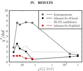
FIG. 1: (Color online)χ2/do f versus√s
NN for the homogeneous (δT =δµ=0, squares) and the inhomogeneous fit (δT andδµfree parameters, circles and triangles). Circles denote the case of local strangeness neutrality, while triangles represent the global strange-ness neutrality case. The lines are meant to guide the eye. Further-more, theχ2/do fcorresponding to the 95.4% confidence interval is shown by the dotted line.
Fig. 1 shows the minimalχ2per degree of freedom (taken
as the number of data points minus the number of parame-ters) for the homogeneous approach and the inhomogeneous approach with local or global strangeness neutrality, respec-tively. Note that theχ2-values for the homogeneous model
are in general agreement with the analysis done in [9] and other data from the literature [10, 11, 33]. As already shown in [14] and in general accordance with the analysis done in [9], for energies,√sNN ≃7.6−17.3 GeV,χ2/do f is consid-erably smaller for the inhomogeneous freeze-out surface than for the homogeneous case, which is far outside the 95.4% confidence interval [35]. At√sNN =6.3 GeV and at RHIC energies,χ2/do f is similar for the inhomogeneous approach
with local strangeness neutrality and the homogenous model. However, between √sNN =6.3 and 12.3 GeV the χ2/do f values for the inhomogeneous approach with local strange-ness neutrality are rather large (between 2 and 4). In contrast, the inhomogeneous model with global strangeness neutrality gives χ2/do f ≈1 for √s
NN =6.3−17.3 GeV. It is impor-tant to note that this result is not due to introducing an addi-tional parameter, but just due to allowing for domains of finite strangeness with global strangeness neutrality! The calcula-tions using global strangeness conservation for RHIC ener-gies are under way, but due to the corresponding small baryon chemical potentials at these high energies no considerable ef-fect should be expected. Thus, the inhomogeneous model al-lowing for domains of finite net strangeness gives a very sat-isfactory description (χ2/do f ≈1) of the experimental data
for particle abundance ratios from lowest SPS energies up to highest RHIC energies. However, at RHIC the homogeneous approach already gives a good description of the data and the inhomogeneous model does not provide a statistically signif-icant improvement. Thus, the assumption of a nearly
homo-geneous decoupling surface can not be rejected there. On the other hand, the considerable improvement of the description of the data for√sNN≃7.6−17.3 GeV indicates that at inter-mediate and high SPS energies, the experimental data favor an inhomogeneous freeze-out surface. For the SPS√sNN =6.3 GeV data the situation is not clear: there is certainly a reduc-tion of theχ2/do f in the inhomogeneous approach, but also
the homogeneous model gives a much better value than for higher SPS energies. Here more experimental data are neces-sary to clarify the picture. It is worth noting that in general, the improvement due to the inhomogeneous decoupling sur-face is not driven by one single species; rather, the inhomo-geneous model describes nearly all multiplicities better than a homogeneous decoupling surface [36].
To illustrate the significance of inhomogeneities differently, we show contours ofχ2/do fin the plane ofδT,δµ
Bin Figs.2, 3, and 4. Here,T andµBwere allowed to vary freely such as to minimizeχ2at each point. Fig. 2 shows that at RHIC
en-ergy,χ2is very flat in both directions. This shows again that
with the present data points, a homogeneous freeze-out model appears to be a reasonable approximation at high energies. In
FIG. 2:χ2/do f contours in theδT,δµ
Bplane for top RHIC energy, (√sNN=200 GeV). The other two parameters (T,µB) are allowed to vary freely. Theχ2/do fminimum is indicated by the cross.
contrast, Fig. 3 shows thatχ2is relatively flat along theδµ
B di-rection, whileδT is determined more accurately and is clearly non-zero. In general we find that in the approach with lo-cal strangeness neutrality there is little correlation betweenδT andδµBand that about the minimum,χ2is rather flat inδµB direction for all energies. Finally, Fig. 3 shows the contours at SPS√sNN =17.3 GeV for the case of global strangeness neutrality. Now, theχ2determines theδµ
FIG. 3: Same as Fig. 2 for top SPS energy (√sNN=17.3 GeV) with local strangeness neutrality.
FIG. 4: Same as Fig. 2 for top SPS energy (√sNN=17.3 GeV) with global strangeness neutrality.
distribution in δµBdirection. In contrast, if the net strange-ness vanishes globally, in domains of high chemical potential resulting from a large width δµB, a large number of strange particles can be produced. Thus, theχ2should be much more
sensitive to the value ofδµB.
As already discussed above, an inhomogeneous freeze-out surface or finite values for the width-parameters result in dif-ferent mean emission temperatures and chemical potentials for different particle species, c.f. eq. 9. These are shown in Fig. 5 for the case of local strangeness neutrality and in Fig. 6 for the case of global strangeness neutrality at selected energies in the CERN-SPS range. For the cases shown, the inhomogeneities determined from the fits to the particle abun-dances are large. Note that the different values for these mean emission temperatures and chemical potentials result from the convolution of the distribution function for a given particle species with the Gaussian probability distribution determined by the four parameters T,µB,δT,δµB. For both cases, the effect of the inhomogeneities is evident. For example, anti-protons are typically emitted from regions with lower baryon-chemical potential than protons; also, heavy particles are con-centrated in “hot spots” while light pions are distributed more evenly throughout the decoupling volume etc. [37]. Figures 5
100 150 200 250 300 350 400 450 500 550 600
µ
B[MeV]
120 140 160 180 200
T
[MeV]
π π
π
K+ K+ K+
K_ K_ K_
p p
p Ω
Ω Ω
Ω Ω Ω
p p p
SPS-40 SPS-80 SPS-158
FIG. 5: (Color online) Freeze-out temperatures Ti and chem-ical potentials µBi of various particle species at √sNN = 8.8,12.3,17.3 GeV (corresponding toELab=40,80,158 GeV) for local strangeness neutrality.
100 200 300 400 500 600
µ
B[MeV]
120 130 140 150 160 170 180 190 200
T
[MeV]
π π
π K+
K+ K+
K_ K_ K_
p p
p
Ω Ω
Ω
Ω Ω Ω
p p
p
SPS-40 SPS-80 SPS-158
FIG. 6: (Color online) Freeze-out temperatures Ti and chem-ical potentials µBi of various particle species at √sNN = 8.8,12.3,17.3 GeV (corresponding toELab=40,80,158 GeV) for global strangeness neutrality.
not the case anymore if the strange chemical potential is deter-mined globally and constant for the different domains. Then, the mean freeze-out points for the different particle species are spread over a much wider range in theT−µB-plane. On the other hand, the spread in temperature is somewhat larger in the local case than for global strangeness neutrality, resulting from the larger best fit values for the width parametersδT.
V. SUMMARY AND OUTLOOK
In summary, we have shown that inhomogeneities on the freeze-out hypersurface do not average out but reflect in the 4π (or midrapidity), single-inclusiveabundances of various particle species. This is due to the non-linear dependence of the hadron densities ρi(T,µB)on the local temperature and baryon-chemical potential. Consequently, even the averageρi
probe higher moments of theT andµBdistributions. In [14] we showed that an inhomogeneous freeze-out model with lo-cal strangeness conservation strongly improves the descrip-tion of the data at medium and top SPS energies compared to the homogeneous freeze-out. Here we showed that induc-ing global strangeness neutrality, results, without addinduc-ing an additional parameter, in a further reduction of theχ2at SPS
energies. With the resultingχ/do f ≈1 for the whole range - from lowest SPS to highest RHIC energies. Furthermore, while for local strangeness neutrality we observed a rather flat
χ2/do f inδµ
Bdirection, this is determined more accurately if strangeness neutrality is ensured only globally. Rather in this approach a high statistical significance for a finite width of the distributions for temperatureandbaryon chemical poten-tial at medium and high SPS energies is observed. In addition we showed how in this region the mean emission temperature and chemical potential vary for different particle species. Our results also show that there are some characteristic differences in the distribution of the resulting mean emission values, de-pending on whether strangeness neutrality is fulfilled locally
or globally. Especially the separation in the mean emission chemical potential between baryons and the corresponding anti-baryons is strongly influenced by the adopted strangeness neutrality condition.
Inhomogeneities could also affect the coalescence proba-bilities of (anti-) nucleons to light (anti-) nuclei, which are also sensitive to density perturbations [39]. Other signals, such as two-particle correlations [8, 40], could also be ana-lyzed in this regard. Future studies should shed more light on whether these inhomogeneities can indeed be interpreted as fingerprints of a first-order phase transition. Eventually, one would want to establish more quantitative relations between the amplitudes of theT,µBinhomogeneities and the proper-ties of the phase transition, e.g. its latent heat and interface tension.
Data from GSI-FAIR, the low energy program at RHIC and and CERN-LHC will provide additional constraints for the evolution of chemical freeze-out with energy.
To improve the quality of the statistical fits, more data on hadron multiplicities would be helpful, in particular at the lower end of the CERN-SPS energy spectrum and at RHIC. This includes estimates of multiplicities of unstable reso-nances (ρ, K∗, ω, ∆ ...) at chemical freeze-out [41]. Data from GSI-FAIR and CERN-LHC will provide additional con-straints for the evolution of chemical freeze-out with energy.
Acknowledgements
We thank A. Dumitru for cooperating in this work, C. Greiner for fruitful remarks concerning the model, C. Blume and M. Gazdzicki for helpful discussions about the NA49 data and A. Grunfeld for helping with the construction of the resonance table, CAPES and CNPq for partial support and the organizers of the ‘II Workshop on Particle Correla-tions and Femtoscopy’ (WPCF 2006), September 9-11, 2006, S˜ao Paulo, Brazil, where this work was presented.
[1] H. St¨ockeret al., Nucl. Phys. A566, 15c (1994); Nucl. Phys. A 590, 271c (1995);
[2] Z. Fodor and S. D. Katz, JHEP0404, 050 (2004).
[3] M. Stephanov, K. Rajagopal, and E. V. Shuryak, Phys. Rev. Lett.81, 4816 (1998).
[4] D. Bower and S. Gavin, Phys. Rev. C64, 051902 (2001). [5] K. Paech and A. Dumitru, Phys. Lett. B 623, 200 (2005);
K. Paech, H. St¨ocker, and A. Dumitru, Phys. Rev. C 68, 044907 (2003); O. Scavenius, A. Dumitru, and A. D. Jackson, arXiv:hep-ph/0103219, Figs. 5,6.
[6] http://map.gsfc.nasa.gov/m_mm.html
[7] M. Gyulassy, D. H. Rischke, and B. Zhang, Nucl. Phys. A613, 397 (1997); M. Bleicheret al., Nucl. Phys. A638, 391 (1998); H. J. Drescher, S. Ostapchenko, T. Pierog, and K. Werner, Phys. Rev. C65, 054902 (2002).
[8] O. J. Socolowski, F. Grassi, Y. Hama, and T. Kodama, Phys. Rev. Lett.93, 182301 (2004).
[9] A. Andronic, P. Braun-Munzinger, and J. Stachel, Nucl. Phys. A772, 167 (2006) [arXiv:nucl-th/0511071].
[10] see for example K. Redlich, J. Cleymans, H. Oeschler, and A. Tounsi, Acta Phys. Polon. B33, 1609 (2002); P. Braun-Munzinger, K. Redlich, and J. Stachel, arXiv:nucl-th/0304013; M. Michalec, arXiv:nucl-th/0112044; and references therein. [11] J. Rafelski, Phys. Lett. B 262, 333 (1991); J. Rafelski,
J. Letessier, and A. Tounsi, Acta Phys. Polon. B 27, 1037 (1996); F. Becattini, J. Cleymans, A. Keranen, E. Suhonen, and K. Redlich, Phys. Rev. C 64, 024901 (2001); F. Becat-tini, M. Gazdzicki, A. Keranen, J. Manninen, and R. Stock, Phys. Rev. C 69, 024905 (2004); G. Torrieri, S. Steinke, W. Broniowski, W. Florkowski, J. Letessier, and J. Rafel-ski, arXiv:nucl-th/0404083; S. Wheaton and J. Cleymans, arXiv:hep-ph/0412031; J. Letessier and J. Rafelski, arXiv:nucl-th/0504028.
[12] F. Becattini, J. Manninen, and M. Gazdzicki, arXiv:hep-ph/0511092.
(2002); D. Zschiesche, G. Zeeb, K. Paech, H. St ¨ocker, and S. Schramm, J. Phys. G30, S381 (2004); K. Paechet al., Acta Phys. Hung. A21, 151 (2004).
[14] A. Dumitru, L. Portugal, and D. Zschiesche, Phys. Rev. C73, 024902 (2006) [arXiv:nucl-th/0511084].
[15] B. Berdnikov and K. Rajagopal, Phys. Rev. D 61, 105017 (2000); K. Paech, Eur. Phys. J. C33, S627 (2004).
[16] A. Dumitru and R. D. Pisarski, Phys. Lett. B504, 282 (2001); Nucl. Phys. A698, 444 (2002).
[17] L. Van Hove, Z. Phys. C21, 93 (1983); M. Gyulassy, K. Ka-jantie, H. Kurki-Suonio, and L. D. McLerran, Nucl. Phys. B 237, 477 (1984); L. P. Csernai and J. I. Kapusta, Phys. Rev. D 46, 1379 (1992).
[18] O. Scavenius, A. Dumitru, E. S. Fraga, J. T. Lenaghan, and A. D. Jackson, Phys. Rev. D63, 116003 (2001); E. S. Fraga and R. Venugopalan, Physica A345, 121 (2004); Braz. J. Phys. 34, 315 (2004).
[19] I. N. Mishustin, Phys. Rev. Lett.82, 4779 (1999).
[20] The investigation of other distributions and also the application of the “superstatistics” approach [42] are under way.
[21] see, for example, J. F. Lara, Phys. Rev. D72, 023509 (2005) for a recent discussion of BBN in an inhomogeneous early uni-verse, and for links to earlier literature.
[22] S. A. Basset al., Phys. Rev. C60, 021902 (1999); Phys. Rev. C61, 064909 (2000); Phys. Lett. B460, 411 (1999); S. Soff, S. A. Bass, and A. Dumitru, Phys. Rev. Lett.86, 3981 (2001); D. Teaney, J. Lauret, and E. V. Shuryak, arXiv:nucl-th/0110037; C. Nonaka and S. A. Bass, arXiv:nucl-th/0510038; T. Hirano, U. W. Heinz, D. Kharzeev, R. Lacey, and Y. Nara, arXiv:nucl-th/0511046.
[23] H. Sorge, Phys. Lett. B373, 16 (1996).
[24] P. Braun-Munzinger, J. Stachel, and C. Wetterich, Phys. Lett. B 596, 61 (2004).
[25] D. Adamovaet al.[CERES Collaboration], Phys. Rev. Lett.90, 022301 (2003).
[26] Section II in J. Cleymans and K. Redlich, Phys. Rev. C 60, 054908 (1999); for the general argument for 4πratios see e.g. eqs. (1-3) in M. Bleicheret al., Phys. Rev. C59, 1844 (1999). [27] P. Braun-Munzinger, I. Heppe, and J. Stachel, Phys. Lett. B465,
15 (1999).
[28] C. H¨ohne (for the NA49 collaboration), nucl-ex/0510049. Our present best fit (of the 4πratios) for the inhomogeneous model without independent fluctuations ofµS yieldsΛ/p=0.93 at ELab/A=40 GeV, for example, versus 0.76 forδT =δµB=0 (without contributions from weak decays).
[29] M. Gazdzickiet al.[NA49 Collaboration], J. Phys. G30, S701 (2004) [arXiv:nucl-ex/0403023]; A. Richard [NA49 Collabora-tion], J. Phys. G31, S155 (2005); C. Blume [NA49 Collabo-ration], J. Phys. G31, S685 (2005) [arXiv:nucl-ex/0411039]; C. Alt et al. [The NA49 Collaboration], J. Phys. G 30, S119 (2004) [arXiv:nucl-ex/0305017]; S. V. Afanasievet al. [The NA49 Collaboration], Phys. Rev. C66, 054902 (2002) [arXiv:nucl-ex/0205002]; T. Anticicet al., Phys. Rev. C69, 024902 (2004); S. V. Afanasievet al., Nucl. Phys. A715, 161 (2003) [arXiv:nucl-ex/0208014]; T. Anticicet al.[NA49 Col-laboration], Phys. Rev. Lett.93, 022302 (2004) [arXiv:nucl-ex/0311024]; C. Meurer [NA49 Collaboration], J. Phys. G30, S1325 (2004) [arXiv:nucl-ex/0406016]; M. Mitrovski [NA49 Collaboration], arXiv:nucl-ex/0406011; C. Alt et al. [NA49 Collaboration], Phys. Rev. Lett.94, 192301 (2005) [arXiv:nucl-ex/0409004]; S. V. Afanasevet al.[NA49 Collaboration], Phys. Lett. B491, 59 (2000); A. Mischkeet al., Nucl. Phys. A715,
453 (2003) [arXiv:nucl-ex/0209002]; V. Friese [NA49 Col-laboration], Nucl. Phys. A698, 487 (2002); S. V. Afanasiev et al. [NA49 Collaboration], Phys. Lett. B 538, 275 (2002) [arXiv:hep-ex/0202037]; S. V. Afanasievet al.[NA49 Collabo-ration], Phys. Lett. B538, 275 (2002) [arXiv:hep-ex/0202037]. [30] J. Adamset al.[STAR Collaboration], arXiv:nucl-ex/0311017; M. Calderon de la Barca Sanchez, arXiv:nucl-ex/0111004; C. Adler et al. [STAR Collaboration], Phys. Rev. Lett. 89, 092301 (2002) [arXiv:nucl-ex/0203016]; C. Adleret al.[STAR Collaboration], Phys. Lett. B 595, 143 (2004) [arXiv:nucl-ex/0206008]; C. Adler et al. [STAR Collaboration], Phys. Rev. C66, 061901 (2002) [arXiv:nucl-ex/0205015]; C. Adler et al. [STAR Collaboration], Phys. Rev. Lett. 87, 262302 (2001) [arXiv:nucl-ex/0110009]; C. Adler et al. [the STAR Collaboration], Phys. Rev. Lett. 86, 4778 (2001) [Erratum-ibid. 90, 119903 (2003)] [arXiv:nucl-ex/0104022]; C. Adler et al., Phys. Rev. C 65, 041901 (2002). J. Castillo [STAR Collaboration], Nucl. Phys. A 715, 518 (2003) [arXiv:nucl-ex/0210032]; J. Adamset al.[STAR Collaboration], Phys. Rev. Lett. 92, 182301 (2004) [arXiv:nucl-ex/0307024]; J. Adams et al. [STAR Collaboration], Phys. Lett. B 567, 167 (2003) [arXiv:nucl-ex/0211024]; C. Suire [STAR Collaboration], Nucl. Phys. A715, 470 (2003) [arXiv:nucl-ex/0211017]. [31] Calculations for finite values ofδµS=0 are under way.
How-ever, checking the influence of global strangeness conservation without adding an additional parameter represents the first step to be taken in this direction.
[32] J. Cleymans, B. K¨ampfer, M. Kaneta, S. Wheaton, and N. Xu, Phys. Rev. C71, 054901 (2005).
[33] O. Barannikova [STAR Collaboration], arXiv:nucl-ex/0403014; J. Adamset al.[STAR Collaboration], arXiv:nucl-ex/0501009; J. Adamset al.[STAR Collaboration], Phys. Rev. Lett.92, 112301 (2004) [arXiv:nucl-ex/0310004];
[34] S. Eidelmanet al.[Particle Data Group Collaboration], Phys. Lett. B592, 1 (2004).
[35] For SPS√sNN=17.3 GeV only the 4πfit is shown; restrict-ing the homogeneous fit to the mid-rapidity data gives smaller
χ2/do f, but still significantly higher than in the inhomogeneous approach.χ2is smaller if other particle ratios are considered, as for exampleΞ/Λ,Ω/Ξinstead ofΞ/π,Ω/π[9] or if finite widths of resonances are taken into account [12]. However, the increase ofχ2at SPS energies is generic if Na49 4π-data are fitted.
[36] D. Zschiesche, arXiv:nucl-th/0505054, Fig. 7.
[37] Note that the rather high temperatures of the hot spots from which the heavy particles emerge might indicate the need for a better treatment of interactions [13] than the simple excluded-volume model employed here.
[38] E. V. Shuryak and M. A. Stephanov, Phys. Rev. C63, 064903 (2001); M. Abdel-Aziz and S. Gavin, Phys. Rev. C70, 034905 (2004).
[39] see e.g. eq. (30) in B. L. Ioffe, I. A. Shushpanov, and K. N. Zyablyuk, Int. J. Mod. Phys. E13, 1157 (2004); [40] H. Heiselberg and A. D. Jackson, arXiv:nucl-th/9809013;
S. J. Lindanbaum, R. S. Longacre, and M. Kramer, arXiv:nucl-th/0304082; W. N. Zhang, S. X. Li, C. Y. Wong, and M. J. Efaaf, Phys. Rev. C71, 064908 (2005).
[41] C. Markert, J. Phys. G31, S169 (2005).