Femtoscopic Correlations in Multiparticle Production and Beta-Decay
R. Lednick´y1,2
1 Joint Institute for Nuclear Research, Dubna, Moscow Region, 141980, Russia 2 Institute of Physics ASCR, Na Slovance 2, 18221 Prague 8, Czech Republic
Received on 11 December, 2006
The basics of formalism of femtoscopic and spectroscopic correlations are given, the orthogonal character of these correlations is stressed. The similarity and difference of femtoscopic correlations in multiparticle production and beta-decay is discussed.
Keywords: Femtoscopy; Correlations; Beta-decay
I. INTRODUCTION
The momentum correlations of two or more particles at small relative momenta in their center-of-mass (c.m.) system are widely used to study space-time characteristics of the pro-duction processes on a level of fm=10−15m, so serving as a correlation femtoscopy tool. Particularly, for non-interacting identical particles, like photons, or to some extent pions, these correlations result from the interference of the production am-plitudes due to the symmetrization requirement of quantum statistics (QS) [1–5].
The momentum QS correlations were first observed as an enhanced production of the pairs of identical pions with small opening angles (GGLP effect [1]). Later on, Kopylov and Podgoretsky settled the basics of correlation femtoscopy in more than 20 papers (see a review [5]) and developed it as a practical tool; particularly, they suggested to study the inter-ference effect in terms of the correlation function, proposed the mixing techniques to construct the uncorrelated reference sample and clarified the role of the space–time characteristics of particle production in various physical situations.
There exists [2–8] an analogy of the momentum QS cor-relations of photons with the space–time corcor-relations of the intensities of classical electromagnetic fields used in astron-omy to measure the angular radii of stellar objects based on the superposition principle (HBT effect) [10]. This analogy is sometimes misunderstood and the momentum correlations are mixed up with space-time (HBT) correlations despite their orthogonal character. The absence of the former in astronomy measurements due to the extremely large space-time extent of stellar objects (and vice versa) was already pointed out in early paper [8] (see also [9]).
Note that though space-time (HBT) correlations are absent in subatomic measurements, they can still be used in the lab-oratory as an intensity-correlation spectroscopy tool allow-ing one to measure the spectral line shape and width (see [11, 12] and references therein). In fact, the QS space-time correlations give information about the shape and width of the three-momentum distribution (including the angular one) of the quanta coming from a distant source and can be consid-ered as a spectroscopy tool in this more general sense.
The momentum correlations of particles emitted at nuclear distances are also influenced by the effect of final state action (FSI) [13–17]. Thus the effect of the Coulomb inter-action dominates the correlations of charged particles at the
relative momenta 2k∗ in the two-particle rest frame smaller than the inverse Bohr radius|a|−1of the two-particle system, respectively suppressing or enhancing the production of parti-cles with like or unlike charges.
Though the FSI effect complicates the correlation analy-sis, it is an important source of information allowing for coa-lescence femtoscopy (see, e.g., [18–21]), and the correlation femtoscopy with unlike particles [15–17], including the ac-cess to the relative space–time asymmetries in particle pro-duction [22–33], and a study of strong interactions between specific particles [29, 32, 33].
In fact, femtoscopic Coulomb correlations were observed more than 70 years ago when the sensitivity of the differential beta-decay rate to the nucleus charge and radius was estab-lished [34].
The paper is organized as follows. In sections II-IV we give the basics of the formalism for femtoscopic and spectroscopic correlations. The similarity and difference of femtoscopic correlations in multiparticle production and beta-decay is dis-cussed in section V. We conclude in section VI. For recent re-sults from femtoscopy of multiparticle production processes, one can inspect several reviews [33, 35–37].
II. FEMTOSCOPIC QS CORRELATIONS
A. Formalism
The correlation function
R
(p1,p2) of two particles with four-momenta p1 and p2 is usually defined as the ratio of the measured momentum distribution of the two particles to the reference one obtained by mixing particles from differ-ent evdiffer-ents of a given class, normalized to unity at sufficidiffer-ently large relative momenta.(i) The multiplicity of produced particles is assumed suffi-ciently large to neglect the influence of conservation laws.
(ii) Independent or incoherent particle emission is assumed, i.e. the coherent contribution of multiparticle emitters is ne-glected (this contribution can be eventually taken into account with the help of the suppression parameterλ).
(iii) The mean freeze-out phase space density is assumed sufficiently small so that the correlation function of two parti-cles emitted with a small relative momentumQ=2k∗in their c.m. system is mainly determined by their mutual correlation. (iv) The momentum dependence of one-particle emission probabilities is assumed inessential when varying the parti-cle four-momentap1andp2by the amount characteristic for the correlation effect. This so-calledsmoothnessassumption requires the components of the mean space-time distance be-tween particle emitters much larger than those of the space-time extent of the emitters.
The probability amplitude to observe a particle with the four-coordinate x from an emitter A decaying at the four-coordinate xA can depend on x through the relative four-coordinatex−xAonly and so can be written in the form:
x|ψA= (2π)−4
d4κuA(κ)exp[iκ(x−xA)]. (1) We assume here that after production the emitter moves along a classical trajectory and decays exponentially. Such a classi-cal treatment of the decay is often applied also to resonances (see, e.g., [39–41]). It is justified for a heavy emitter with the energy spectrum of the decay particle substantially wider than the emitter width. One can avoid the classical treatment of the emitter decay by consideringxAin Eq. (1) as the emitter pro-duction (excitation) four-coordinate and adding, in the case of a negligible emitter space-time extent, the theta-function
θ(t−tA).
The probability amplitude to observe a particle with the four-momentumpis
p|ψA=
d4xp|xx|ψA=uA(p)exp(−ipxA), (2) wherep|x=exp(−ipx). The probability amplitude to ob-serve identical spin-0 bosons with four-momenta p1 and p2 emitted by emitters A and B should be symmetrized in accor-dance with the requirement of QS:
TABsym(p1,p2) = [p1|ψAp2|ψB+p2|ψAp1|ψB]/
√ 2.
(3) The corresponding QS correlation function is given by the properly normalized square of this amplitude averaged over all characteristics of the emitters:
R
(p1,p2) =1+ℜ ∑ABuA(p1)uB(p2)u∗A(p2)u∗B(p1)exp(−iq∆x) ∑AB|uA(p1)uB(p2)|2
.
=1+cos(q∆x), (4)
whereq=p1−p2,∆x=xA−xBand the last equality follows from thesmoothnessassumption (iv).
It should be noted that the last equality in Eq. (4) is usually used to calculate correlation functions within classical trans-port models identifying the emitter four-coordinates as those of the decay four-coordinates of the primary emitters includ-ing resonances or those of the last collisions of the emitted particles. Concerning the accuracy of the classical approach to the emitter decay, we note that, for example in the case of a
ρ-meson and a pion emitted from a small space-time region, it is a valid approximation atQ<0.1 GeV/cbut overestimates the tail of the corresponding two-pion correlation function by about 15 percent (see Fig. 2 in [39]). This overestimation is however not important when the space-time separation of the emitters is larger than 2 fm (as in heavy ion collisions) and so the interference effect rapidly vanishes atQ>0.1 GeV/c.
It is instructive to introduce the emission functionG(x¯,p) (similar to Wigner function) as a partial Fourier transform of the space-time density matrix:
G(x¯,p) =
d4εexp(−ipε)
∑
A
x+¯ 1
2ε|ψAψA|x¯− 1 2ε. (5)
Since the single-particle emission probability is given by the integral
d4x G(¯ x¯,p) =
∑
A
|p|ψA|2, (6)
the emission function, though not positively defined, can be usually interpreted as a probability density to find a particle with four-momentum p and an average four-coordinate ¯x=
1
2(x+x′). For the QS correlation function of two identical spin-0 bosons one has:
R
(p1,p2) =1+d4x¯1d4x¯2G(x¯1,p)G(x¯2,p)cos(q∆x)¯
d4x¯
1d4x¯2G(x¯1,p1)G(x¯2,p2)
.
=1+cos(q∆x)¯, (7)
where∆x¯=x¯1−x¯2andp=12(p1+p2)≡12P. Similar to Eq. (4), the last equality follows from thesmoothnessassumption allowing one to identify the average four-coordinate ¯xof the emitted particle with the decay four-coordinate of its emitter, i.e. neglect the space-time extent of the emitter.
Generally, for two identical bosons or fermions with total spinS, the ”+” sign in Eq. (3) should be substituted by(−1)S
or, equivalently, the two-particle amplitude should be sym-metrized (anti symsym-metrized) only for identical bosons (fermi-ons) emitted with the same spin projections. As a result, in the case of initially unpolarized spin-jparticles, the ”+” sign in Eq. (4) or (7) for the QS correlation function should be substituted by(−1)2j/n
j, wherenjis the number of possible
spin projections:nj=2j+1 or, for massless particles,nj=2.
of randomly oriented one-photon dipole or quadrupole emit-ters, it equals 14(1+cos2θ)or 41(1−3 cos2θ+4 cos4θ), re-spectively [43]. However, in the case of practical interest, when the photon wavelength is essentially smaller than the size of the photon emission region, the angleθbetween pho-tons contributing to the interference effect is very small and the spin factor reduces to the value 1/nj=12 irrespective of
the multipole order of the emitter.
The correlation function of neutral kaons also deserves comment. Two neutral kaons with four-momenta p1 and p2 are originally produced as pairs K0(p1)K0(p2),
¯ K0(p
1)K¯0(p2),K0(p1)K¯0(p2)and ¯K0(p1)K0(p2). The cor-relation pattern now depends on the way the neutral kaons are detected. In principle, one can detectK0and ¯K0, e.g., by charge exchange reactionsK0→K+and ¯K0→K−. In this case, only the first two production channels would give the interference effect similar to that for identical pions. Usually, however, neutral kaons are detected through their two-pion and three-pion decays as so-called short-lived (K0
S) and
long-lived (KL0) states, respectively. Neglecting the small effect of CP-violation, these states correspond to the eigen states with CP=±1:
|KS0= (|K0+|K¯0)/√2, |KL0= (|K0 − |K¯0)/√2. (8) Therefore, all four production channels of the pairs of K0- and ¯K0-mesons contribute to the production of the pairs KS0(p1)KS0(p2), KL0(p1)KL0(p2), KS0(p1)KL0(p2) and
KL0(p1)KS0(p2). It is clear that the channels K0(p1)K0(p2) and ¯K0(p1)K¯0(p2)yield the constructive interference pattern for any combination of the detected pairs of KS0- and KL0 -mesons. It is interesting that also the channelsK0(p1)K¯0(p2) and ¯K0(p1)K0(p2)now yield the interference effect which can be both constructive and destructive. Indeed, since there are two indistinguishable amplitudes contributing to final state, the symmetrized amplitude has the form [44]:
TABsym(K0
i(p1),K0j(p2))
= Ki0|K0K0j|K¯0p1|ψA(K0)p2|ψB(K¯0)
+K0j|K0Ki0|K¯0p2|ψA(K0)p1|ψB(K¯0), (9) where the sign ”+” corresponds to Bose statistics of neutral kaons. One may see that the corresponding interference pat-tern is constructive forKS0KS0- andKL0KL0-pairs while it is de-structive forKS0KL0-pairs.
B. Simple parameterizations
A characteristic feature of the QS correlation function of two identical bosons (fermions) is the presence of the inter-ference maximum (minimum) at small components of the rel-ative four-momentumqwith the width reflecting the inverse space-time extent of the effective production region. For ex-ample, assuming that for a fractionλ of pion pairs, the pi-ons are emitted independently according to one–particle am-plitudes of a Gaussian form characterized by the space–time dispersionsr02 andτ2
0, while the remaining fraction(1−λ)
relates to very long–lived emitters (η,η′,K0
s,Λ, . . . ). Since
the relative distancesr∗between the emitters in this remaining fraction in the pair c.m. system are extremely large, one has
R
(p1,p2) =1+λexp
−r20q2−τ2 0q20
=1+λexp−r20q2T−(r02+v2τ20)q2L
,(10)
whereqT andqL are the transverse and longitudinal
compo-nents of the three–momentum differenceqwith respect to the direction of the pair velocityv=P/P0. One may see that, due to the on-shell constraint [3]q0=vq≡vqL (following from
the equalityqP=0), strongly correlating the energy differ-enceq0 with the longitudinal momentum differenceqL, the
correlation function atvτ0>r0substantially depends on the direction of the vectorq, even in the case of a spherically sym-metric spatial form of the production region.
Note that the on-shell constraint makes theq-dependence of the correlation function essentially three–dimensional and thus makes it impossible to find a unique Fourier recon-struction of the space–time characteristics of the emission process. Particularly, in the pair c.m. system,q={0,2k∗},
∆x={t∗,r∗}) and the scalar productq∆x=−2k∗r∗is inde-pendent of the time differencet∗. However, within realistic models, the directional and velocity dependence of the corre-lation function can be used to determine both the duration of the emission and the form of the emission region [3], as well as - to reveal the details of the production dynamics (such as collective flows; see,e.g., [45, 46] and the reviews [47, 48]). For this, the correlation functions can be analyzed in terms of the out (x), side (y) and longitudinal (z) components of the rel-ative momentum vectorq={qx,qy,qz}[49, 50]; the out and
side denote the transverse, with respect to the reaction axis, components of the vector q, the out direction is parallel to the transverse component of the pair three–momentum. The corresponding correlation widths are usually parameterized in terms of the Gaussian correlation radiiRi,
R
(p1,p2) =1+λexp(−R2xq2x−R2yq2y−R2zqz2−R2xzqxqz)(11) and their dependence on pair rapidity and transverse momen-tum is studied. The form of Eq. (11) assumes azimuthal sym-metry of the production process [47, 49]. Generally,e.g., in case of the correlation analysis with respect to the reaction plane, all three cross termsqiqjcontribute [51].
componentqx=γtq∗x, whereγtis the LCMS Lorentz factor of
the pair.
Particularly, in the case of one–dimensional boost invariant expansion, the longitudinal correlation radius in the LCMS reads [46]Rz≈(T/mt)1/2τ, whereTis the freeze-out
temper-ature,τis the proper freeze-out time andmt is the transverse
particle mass. In this model, the side radius measures the transverse radius of the system while, similarly to Eq. (10), the square of the out radius gets an additional contribution (pt/mt)2∆τ2due to the finite emission duration∆τ. The
ad-ditional transverse expansion leads to a slight modification of the pt–dependence of the longitudinal radius and - to a
no-ticeable decrease of the side radius and the spatial part of the out radius withpt. Since the freeze-out temperature and the
transverse flow also determine the shapes of themt-spectra,
the simultaneous analysis of correlations and single particle spectra for various particle species allows one to disentangle all the freeze-out characteristics [47].
III. SPECTROSCOPIC QS CORRELATIONS
To help in understanding the analogy and difference of QS space-time (spectroscopic) and momentum (femtoscopic) cor-relations, we briefly present the formalism of QS correla-tion spectroscopy within the KP model of independent single-particle emitters. In spectroscopic correlation measurements the particles are supposed to be emitted by a distant object with large space-time dimensions and detected by two detec-tors at space-time pointsx1andx2. It is assumed that the dis-tance between the detectors is much smaller than the size of the emitting object and that this size is negligible compared with the distance between the object and detectors. Then, the four-momentum of a photon emitted by the emitter A and detected by any of the two detectors can be written as pA=ωA{1,pˆA}, where ˆpAis the unit vector in the direction from the emitter A to the detectors. The four-dimensional in-tegral in the single-photon probability amplitude in Eq. (1) then reduces to the one-dimensional one:
x|ψA= (2π)−1
dωAuA(ωA)exp[ipA(x−xA)]θ(t−tA), (12) whereuA(ωA)∝(ωA−ω0A−iΓA)−1, i.e. the emitter decay is treated quantum-mechanically and parameterized by the en-ergyω0A and widthΓA of the emission line. In accordance with the comment after Eq. (1),xAnow denotes the excitation four-coordinate of the emitter and the conditiont>tAis intro-duced by the theta-function. Since the timetAis distributed in a very wide interval, the sum∑Aexp[−i(ωA−ω′A)tA]yields the delta-functionδ(ωA−ω′A)so that the single-photon prob-ability is merely proportional to the integral of the spectral function:
∑
A|x|ψA|2∝
∑
A
dωA|uA(ωA)|2. (13)
The probability amplitude of two photons with the same and complete polarization should be symmetrized similar to Eq.
(3):
T
ABsym(x1,x2) = [x1|ψAx2|ψB+x2|ψAx1|ψB]/√ 2.
(14) For photons with polarizationP, the symmetrized amplitude (14) describes only the fraction12(1+P2)of the photon pairs. As a result, the correlation function
R
(x1,x2), defined as a number of two-photon counts normalized to unity at a large space-time separation of the detected photons, becomesR
(x1,x2) =1+ 1+P22 ·
·∑AB
dωAdωB|uA(ωA)|2|uB(ωB)|2cos(qAB∆x) ∑AB
dωAdωB|uA(ωA)|2|uB(ωB)|2
=1+1+P
2
2 cos(qAB∆x), (15) whereqAB=pA−pB,∆x=x1−x2.
It should be noted that the HBT technique is not based on counting separate quanta. Instead, it overcomes this diffi-cult problem by the measurement of the product of fluctuat-ing parts of the electric currents from the two detectors (the low-frequency part is filtered out) integrated and read in time intervals of the order of minutes. To get rid of the uncertainties in the detector gains the measured quantity is the ratio of the product mean to root-mean-square deviation. It can be shown that the correlation coefficient defined as this ratio normalized to unity at zero distance between the detectors, equals to
cos(qAB∆x) ≈[2J1(ρ)/ρ]2. (16) The approximate equality is valid for a uniformly radiating disk with the normal directed to the detectors (or, for a spher-ical surface radiating according to Lambert’s law) emitting light of a small band width; the argument of Bessel function J1isρ=ωθ¯ d, where ¯ωis the mean angular frequency (mean energy of the detected photons),dis the distance between the detectors perpendicular to the direction to the distant emitting object andθis the object angular radius. Measuring the cor-relation coefficient as a function of the distanced, one thus determines the transverse spread ¯ωθof the wave vectors of the detected light (the spread of the transverse photon mo-menta). Obviously, the HBT correlation effect is insensitive to the actual space-time extent of the source. At most, one can determine the source angular radiusθperforming the ad-ditional spectral measurements of the mean angular frequency
¯
ω.
It is interesting to note that Eq. (16) follows also from the superposition principle applied to classical electromagnetic fields and so the HBT intensity correlation effect would sur-vive even in the case of vanishing Planck constant when the QS correlations become unobservable.
Some historical remarks are appropriate here. The analogy of QS momentum correlations with HBT space-time correla-tions was first mentioned in paper [2]. However, not stressing the differences, this paper triggered a number of misleading statements, such as [6]: ”The interest to correlations of identi-cal quanta is due to the fact that their magnitude is connected with the space and time structure of the source of quanta. This idea originates from radio astronomy and is the basis of Hanbury-Brown and Twiss method of the measurement of star radii”. To clarify the situation, Kopylov and Podgoretsky wrote a special paper [8] in which they clearly stressed the difference between the momentum and space-time QS corre-lation measurements. Particularly, they pointed out: ”when any of the time parameters characterizing radiating system becomes very large, the possibility to measure the system di-mensions practically vanishes since the interference effect re-mains only in the unobservable small region of the energy dif-ference q0. On the other hand, in astronomy, it appears to be
possible to measure angular dimensions of stars despite their lifetimes can be considered infinitely large”. Unfortunately, this clarifying paper missed the attention of a number of ex-perts in the field of interference correlations. Thus even in reviews on the subject one can meet the incorrect statement that there is no principle difference between QS correlations in particle physics and astronomy, that both are momentum correlations allowing one to determine spatial dimensions of the emitting object. An example of such incorrect view of QS correlations in astronomy is given in Fig. 1 [53]. Another ex-ample of this widespread error is chapter 1.1 in a review [54].
correla-tion
d
star
b
p
1p
21
a
2
q
FIG. 1: An example of the incorrect view of spectroscopic QS correlations in astronomy [53]. Neither the extremely small three-momentum differenceqbetween the photons from the same emitter (a negligible part of the photon pairs) nor the one between the pho-tons from different emitters can directly be measured in astronomy. In fact, this figure would be a correct view of femtoscopic QS corre-lations if a distant star were substituted by a nearby object emitting identical particles at a characteristic space-time distance of the order of femtometer.
IV. FEMTOSCOPIC FSI CORRELATIONS
It can be shown [14, 15, 55] that the effect of FSI man-ifests itself in the fact that the role of a functional basis, which the asymptotic two-particle state is projected onto, is transferred from plane waves exp(−ip1x1−ip2x2) to the Bethe-Salpeter amplitudes Ψ(p−1)p2(x1,x2) = Ψ
(+)∗
p1p2(x1,x2) =
exp(−iPX)ψ(+)q˜ ∗(∆x), where∆x≡x1−x2={t,r}is the rela-tive four-coordinate,q=q−P(qP)/P2is the generalized rel-ative four-momentum,P=p1+p2andqP=m12−m22.
To simplify the calculation of the FSI effect, the Bethe-Salpeter amplitude describing two particles emitted at space-time points xi={ti,ri} and detected with four-momenta pi is usually calculated at equal emission times in the pair c.m. system; i.e. the reduced non-symmetrized Bethe-Salpeter am-plitudeψ(+)q˜ (∆x)is substituted in the two-particle c.m. sys-tem, whereP=0, ˜q={0,2k∗}and∆x={t∗,r∗}), by a sta-tionary solutionψ(+)−k∗(r∗)of the scattering problem having at
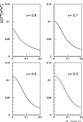
large distancesr∗ the asymptotic form of a superposition of the plane and outgoing spherical waves (the minus sign of the vectork∗ corresponds to the reverse in time direction of the emission process). Thisequal timeapproximation is valid for conditions [15, 55]|t∗| ≪m2,1r∗2. These conditions are usu-ally satisfied for heavy particles like kaons or nucleons. But even for pions, thet∗=0 approximation merely leads to a slight overestimation (typically<5%) of the strong FSI ef-fect (see Fig. 2 and [55]), and it doesn’t influence the leading zero–distance (r∗≪ |a|) effect of the Coulomb FSI.
Note that for small k∗, the case we are interested in, the short-range interaction is dominated by central forces and s-waves so that, neglecting a weak spin dependence of the Coulomb interaction, the spin dependence of the two-particle amplitude enters only through the total spinS.
On the assumptions (i)-(iv), the two-particle correlation function then reduces to the square of the two-particle wave function averaged over the distancer∗ of the emitters in the two-particle c.m. system and the total spinSof the pair:
R
(p1,p2)=. |ψ−(+)k∗(r∗)|2. (17)For identical particles, the amplitude in Eq. (17) enters in a symmetrized form:
ψ(+)−k∗(r∗)→[ψ(+)−k∗(r∗) + (−1)Sψ(+)k∗ (r∗)]/
√
2. (18)
FIG. 2: The FSI contribution to theπ0π0correlation function calcu-lated for the pair velocityv=0.3,0.5,0.7,0.9cin a model of inde-pendent single–particle emitters distributed according to a Gaussian law with the spatial and time width parametersr0=2 fm andτ0=2 fm/c. The exact results (solid curves) are compared with those ob-tained in the equal–time approximation (dash curves).
and inelastic transition amplitudes should be taken into ac-count in the averaging in Eq. (17). In practice, the particles 1,3 and 2,4 are members of the same isomultiplets (as, e.g., in the transitionπ−p→π0nor K+K−→K0K¯0) so that one can assume the same weights and samer∗-distributions for the channels 1+2 and 3+4.
In heavy ion collisions, the effective radiusr0of the emis-sion region can be considered much larger than the range of the strong interaction potential. The short range FSI contribu-tion to the correlacontribu-tion funccontribu-tion is then independent of the ac-tual potential form [15, 57]. At smallQ=2k∗, it is determined by the s-wave scattering amplitudes fS(k∗) at a given total spinSscaled by the radiusr0[15]. For two-nucleon systems, the scattering lengths fS(0)are large (up to∼20 fm) and this contribution often dominates over the effect of QS. For two-meson or two-meson-baryon systems, the scattering amplitudes are usually quite small (<0.2 fm) and the short range FSI contribution (including the contribution of the coupled chan-nel which is quadratic in the amplitude of the corresponding inelastic transition) can be often neglected. This contribution
cannot be however neglected for theKK¯-system due to rather large s-wave KK¯ scattering length dominated by the imagi-nary part of ∼1 fm generated by near-threshold resonances f0(980)anda0(980)[15]. It has been recently shown that the neglect of the FSI contribution in the analysis of the two-KS0 correlation function in Au+Au collisions at√sNN=200 GeV would lead to a noticeable (∼25%) overestimation of the cor-relation radius [58].
V. FEMTOSCOPIC CORRELATIONS IN BETA-DECAY
Let us now consider beta-decay of a nucleus with charge numberZ0, four-momentump0, helicityλ0to a nucleus with charge numberZ, four-momentum p, helicityλ, an electron (positron) with four-momentumpe, helicityλeand an antineu-trino (neuantineu-trino) with four-momentumpν, helicityλν. Taking into account the point-like character of the weak interaction, the equal emission times of the decay particles and the fact that the c.m. system of the electron and final nucleus practi-cally coincides with the rest frame of the initial nucleus (i.e. xZ=. xZ0=0 andk∗
.
=pe), one can write the differential decay rate in the form:
d5w=. ∑λ′s
d3pd3ped3pνδ4(p0−p−pe−pν)· ·d3x
T
(x;λ′s)exp(ipνx)ψ(+)∗−k∗(x)
2
.
=∑λ′sd3k∗d3pνδ(ω0−ω−ωe−ων)d3xd3x′· ·
T
(x;λ′s)T
∗(x′;λ′s)exp[ipν(x−x′)]ψ(+)−k∗∗(x)ψ(+)−k∗(x′),(19)where the amplitude
T
(x;λ′s)is basically determined by the distribution of the decaying neutron (proton) within the nu-cleus.It is instructive to consider the hypothetical situation when the energy release in the decay is large and additional particles are emitted. Then one could neglect energy-momentum con-servation and get, after the integration over the neutrino three-momentum (leading to delta-functionδ3(x−x′)), a similar re-sult as in the case of multiparticle production using conditions (i)-(iv):
d3w d3k∗∝
d3x
∑
λ′s
T
(x;λ′s)ψ(+)−k∗∗(x)
2
∝ψ(+)−k∗(x)
2
.
(20) The actual energy release in beta-decay is however very small so that the integration over the neutrino three-momentum does not lead to the diagonalization of the spatial density matrix
∑λ′s
T
(x;λ′s)T
∗(x′;λ′s). In fact, in so-called allowed decays, the neutrino plane wave exp(ipνx)can be even substituted by unity. Nevertheless, similar results as in Eq. (20) have been obtained by Fermi [34] due to the fact that the relativistic Coulomb wave functionψ(+)−k∗∗(x)of the electron2
4
6
8
k
MeV
c
5
10
15
20
25
F
k
,
Z
,
R
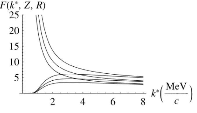
FIG. 3: The Fermi functionF(k∗,Z,R)for beta-decay to a final nucleus of chargeZ=83 as a function of the electron (decreasing curves) or positron momentumk∗and the nucleus radiusR=2,4,8 fm (in decreasing order).
can write in the nucleus rest frame (ω0=M0):
d3w d3k∗
.
=4πF(k∗,Z,R)(M0−M−ωe)2
∑
λ′s
d3x
T
(x;λ′s)
2
,
(21) where
F(k∗,Z,R)=. |ψ(+)−k∗(r∗)|2=. |ψ(+)−k∗(R)|2
.
= (2k∗R)2σ 2σ+4
[Γ(2σ+3)]2exp(−πη)|Γ(σ+1−iη)| 2,(22)
η =. ∓Ze2ωe/k∗ for electrons (positrons), σ = (1 −
Ze2)1/2− 1. The substitution of the separationr∗by the nu-cleus radiusRin the second equality in Eq. (22) is justified due to a weakr∗-dependence of the wave function within the nucleus [34]; the third equality neglects the screening effect of the atomic electrons.
One may see that the nucleus radius enters in the Fermi function through the factor(2k∗R)2σwhich is essentially dif-ferent from unity only for sufficiently large charge numbersZ. At smallZ-values,σ=. 0 and the Fermi function reduces to the
Coulomb penetration (Gamow) factorAc(η) =|ψ−(+)k∗(0)|2=
2πη[exp(2πη)−1]−1. The sensitivity of the Fermi function to the nucleus radius is demonstrated in Fig. 3.
VI. CONCLUSIONS
We have considered femtoscopic QS and FSI momentum correlations in multiparticle production and beta-decay, as well as spectroscopic QS space-time correlations in the de-tected radiation from a distant source. We have demonstrated the orthogonal character of the femtoscopic and spectroscopic correlations, earlier pointed out by Kopylov and Podgoretsky [8]. We have shown that the same functional form of the two-particle correlation function in multitwo-particle production and Fermi function in beta-decay (both being equal to the aver-age square of the two-particle wave function) is due to differ-ent reasons. In the former case, this result is valid in the ap-proximation of independent classical quasi-point-like particle emitters and sufficiently small freeze-out phase space density, while in the latter case it follows from a weak variation of the electron (positron)-nucleus wave function within the nucleus volume and a point-like character of beta-decay. It should be stressed that a small space-time extent of the emitters alone does not guarantee the validity of the approximation of classi-cal emitters (the diagonalization of the space-time density ma-trix). This approximation may naturally be justified in high-energy multiparticle processes due to the minor importance of conservation laws in this case.
Acknowledgments
This work was supported by the Grant Agency of the Czech Republic under contract 202/07/0079 and partly car-ried out within the scope of the GDRE: Heavy ions at ultra-relativistic energies - a European Research Group comprising IN2P3/CNRS, EMN, University of Nantes, Warsaw Univer-sity of Technology, JINR Dubna, ITEP Moscow and BITP Kiev.
[1] G. Goldhaber, S. Goldhaber, W. Lee, and A. Pais, Phys. Rev. 120, 300 (1960).
[2] V.G. Grishin, G.I. Kopylov, and M.I. Podgoretsky, Sov. J. Nucl. Phys.13, 638 (1971).
[3] G.I. Kopylov and M.I. Podgoretsky, Sov. J. Nucl. Phys.15, 219 (1972).
[4] G.I. Kopylov, Phys. Lett. B50, 472 (1974). [5] M.I. Podgoretsky, Sov. J. Part. Nucl.20, 266 (1989). [6] E.V. Shuryak, Phys. Lett. B44, 387 (1973). [7] G. Cocconi, Phys. Lett. B49, 459 (1974).
[8] G.I. Kopylov and M.I. Podgoretsky, Sov. Physics JETP42, 211 (1975).
[9] V.L. Lyuboshitz, Proc. CRIS’98, Acicastello, Italy, 1998, p. 213.
[10] R. Hanbury-Brown and R.Q. Twiss, Nature178, 1046 (1956). [11] M.L. Goldberger, H.W. Lewis, and K.M. Watson, Phys. Rev.
142, 25 (1966).
[12] D.T. Phillips, H. Kleiman, and S.P. Davis, Phys. Rev.153, 113 (1967).
[13] S.E. Koonin, Phys. Lett. B70, 43 (1977).
[14] M. Gyulassy, S.K. Kauffmann, and L.W. Wilson, Phys. Rev. C 20, 2267 (1979).
[15] R. Lednicky and V.L. Lyuboshitz, Sov. J. Nucl. Phys.35, 770 (1982); Proc. CORINNE 90, Nantes, France, 1990 (ed. D. Ar-douin, World Sci., 1990) p. 42.
[16] D.H. Boal and J.C. Shillcock, Phys. Rev. C33, 549 (1986). [17] D.H. Boal, C.-K. Gelbke, and B.K. Jennings, Rev. Mod. Phys.
[18] H. Sato and K. Yazaki, Phys. Lett. B98, 153 (1981). [19] V.L. Lyuboshitz, Sov. J. Nucl. Phys.48, 956 (1988).
[20] S. Mrowczynski, Phys. Lett. B277, 43 (1992); ibid. B308, 216 (1993).
[21] R. Scheibl and U. Heinz, Phys. Rev. C59, 1585 (1999). [22] R. Lednicky, V.L. Lyuboshitz, B. Erazmus, and D. Nouais,
Phys. Lett. B373, 30 (1996).
[23] B. Erazmus et al., CERN Note ALICE-INT-1995-43.
[24] S. Voloshin, R. Lednicky, S. Panitkin, and N. Xu, Phys. Rev. Lett.79, 4766 (1997).
[25] D. Ardouin et al., Phys. Lett. B446, 191 (1999). [26] R. Lednicky, S. Panitkin, and N. Xu, nucl-th/0304062. [27] R. Lednicky, nucl-th/0304063, 0304064.
[28] D. Miskowiec et al. (E877), nucl-ex/9808003.
[29] R. Lednicky, NA49 Note number 210 (1999); nucl-th/0112011, 0212089.
[30] Ch. Blume et al. (NA49), Nucl. Phys. A715, 55c (2003). [31] J. Adams et al. (STAR), Phys. Rev. Lett.91, 262302 (2003). [32] A. Kisiel (STAR), J. Phys. G30, S1059 (2004).
[33] R. Lednicky, Phys. Atom. Nucl.67, 72 (2004).
[34] E. Fermi, Z. Phys.88, 161 (1934); F.L. Wilson, Am. J. Phys. 36, 1150 (1968).
[35] M. Lisa, S. Pratt, R. Soltz, and U. Wiedemann, Ann. Rev. Nucl. Part. Sci.55, 357 (2005).
[36] T. Cs¨org˝o, nucl-th/0505019.
[37] R. Lednicky, Nucl. Phys. A774, 189 (2006).
[38] Yu.M. Sinyukov, R. Lednicky, S.V. Akkelin, J. Pluta, and B. Erazmus, Phys. Lett. B432, 248 (1998).
[39] R. Lednicky and T.B. Progulova, Z. Phys. C55, 295 (1992). [40] R. Lednicky and V.L. Lyuboshitz, Heavy Ion Physics 3, 93
(1996).
[41] S. Cheng and S. Pratt, Phys. Rev. C63, 054904 (2001). [42] D. Neuhauser, Phys. Lett. B182, 289 (1986).
[43] V.L. Lyuboshitz, M.I. Podgoretsky, Phys. Atom. Nucl.58, 30
(1995); V.L. Lyuboshitz, http://www.itep.ru/ions/GDRE/Dubna -ITEP-March-2006/GDRE Dubna Itep March2006.html. [44] V.L. Lyuboshitz, M.I. Podgoretsky, Sov. J. Nucl. Phys.30, 407
(1979).
[45] S. Pratt, Phys. Rev. Lett.53, 1219 (1984); Phys. Rev.D33, 1314 (1986); S. Pratt, T. Cs¨org¨o, and J. Zimanyi, Phys. Rev. C42, 2646 (1990).
[46] A.N. Makhlin and Yu.M. Sinyukov, Yad. Fiz.46, 637 (1987); Z. Phys. C39, 69 (1988); Yu.M. Sinyukov, Nucl. Phys. A498, 151c (1989).
[47] U.A. Wiedemann and U. Heinz, Phys. Rept.319, 145 (1999). [48] T. Cs¨org¨o, Heavy Ion Phys.15, 1 (2002).
[49] M.I. Podgoretsky, Sov. J. Nucl. Phys.37, 272 (1983); R. Led-nicky, JINR B2-3-11460, Dubna (1978); P. Grassberger, Nucl. Phys. B120, 231 (1977).
[50] G.F. Bertsch, P. Danielewicz, and M. Herrmann, Phys. Rev. C 49, 442 (1994); S. Pratt, in Quark Gluon Plasma 2 (ed. R.C. Hwa), World Scientific, Singapore, 1995, p.700; S. Chap-man, P. Scotto, and U. Heinz, Phys. Rev. Lett.74, 4400 (1995). [51] U.A. Wiedemann, Phys. Rev. C57, 266 (1998).
[52] T. Cs¨org¨o and S. Pratt, Proc. Workshop on Heavy Ion Physics, KFKI-1991-28/A, p.75.
[53] P. Grassberger, Proc. VIII-th International Symposium on Mul-tiparticle Dynamics, Kaysersberg, France, June 12-17, 1977. [54] W. Bauer, C-K. Gelbke, and S. Pratt, Annu. Rev. Nucl. Part. Sci
42, 77 (1992).
[55] R. Lednicky, nucl-th/0501065.
[56] R. Lednicky, V.V. Lyuboshitz, and V.L. Lyuboshitz, Phys. Atom. Nucl.61, 2050 (1998).
[57] M. Gmitro, J. Kvasil, R. Lednicky, and V.L. Lyuboshitz, Czech. J. Phys. B36, 1281 (1986).
![FIG. 1: An example of the incorrect view of spectroscopic QS correlations in astronomy [53]](https://thumb-eu.123doks.com/thumbv2/123dok_br/18982397.457524/5.892.91.432.628.860/fig-example-incorrect-view-spectroscopic-qs-correlations-astronomy.webp)