Research Article
Nonlinear Resonance Analysis of Slender Portal Frames under
Base Excitation
Luis Fernando Paullo Muñoz,
1Paulo B. Gonçalves,
1Ricardo A. M. Silveira,
2and Andréa Silva
21Civil Engineering Department, Pontifical Catholic University of Rio de Janeiro, Rio de Janeiro, RJ, Brazil 2Civil Engineering Department, Federal University of Ouro Preto, Ouro Preto, MG, Brazil
Correspondence should be addressed to Luis Fernando Paullo Mu˜noz; [email protected] Received 22 November 2016; Accepted 16 February 2017; Published 30 March 2017
Academic Editor: Marcello Vanali
Copyright © 2017 Luis Fernando Paullo Mu˜noz et al. This is an open access article distributed under the Creative Commons Attribution License, which permits unrestricted use, distribution, and reproduction in any medium, provided the original work is properly cited.
The dynamic nonlinear response and stability of slender structures in the main resonance regions are a topic of importance in structural analysis. In complex problems, the determination of the response in the frequency domain indirectly obtained through analyses in time domain can lead to huge computational effort in large systems. In nonlinear cases, the response in the frequency domain becomes even more cumbersome because of the possibility of multiple solutions for certain forcing frequencies. Those solutions can be stable and unstable, in particular saddle-node bifurcation at the turning points along the resonance curves. In this work, an incremental technique for direct calculation of the nonlinear response in frequency domain of plane frames subjected to base excitation is proposed. The transformation of equations of motion to the frequency domain is made through the harmonic balance method in conjunction with the Galerkin method. The resulting system of nonlinear equations in terms of the modal amplitudes and forcing frequency is solved by the Newton-Raphson method together with an arc-length procedure to obtain the nonlinear resonance curves. Suitable examples are presented, and the influence of the frame geometric parameters and base motion on the nonlinear resonance curves is investigated.
1. Introduction
Lightweight framed structures are extensively used in engi-neering applications such as buildings, industrial construc-tions, off-shore platforms, and aerospace structures. In civil engineering, framed metal structures such as gabled frames are efficient structural forms to withstand various loads such as live, snow, wind, earthquake, and crane loads. Linear models are usually used for the design of these structures. However, as its slenderness increases, the degree of geometric nonlinearity increases as well as the occurrence of instability phenomena. Under dynamic loads, slender frames may be subjected to unwanted (or unsafe) large vibration amplitudes and accelerations and dynamic jumps in the main resonance regions due to hardening or softening frequency-amplitude relation and modal couplings. Therefore, an accurate non-linear dynamic analysis is required. Recent earthquakes have increased the interest in the development of reliable
analytical methods of assessing the dynamic response of existing structures and, if necessary, developing effective retrofit strategies. So, understanding the nonlinear dynamics of framed structures under base excitation constitutes an essential step for their safe design.
The seminal works by Koiter [1] and Roorda [2] have shown the complex postbucking paths exhibited by slender frames; subsequently, several authors have studied the non-linear behavior of reticulated structures liable to buckling under prescribed loading conditions. A compilation of these first results can be found in Bazant and Cedolin [3] who summarize many topics about the stability of slender frames. Design prescriptions are found, for example, in Galambos [4]. More recently, Silvestre and Camotim [5] presented a semianalytical method to analyze the geometrically nonlinear behavior of plane frames, including the influence of eventual buckling mode interaction phenomena. Later, they presented the results concerning the elastic in-plane stability and
second-order behavior of unbraced single-bay pitched-roof steel frames and proposed a methodology to design this type of commonly used structure. In particular, they showed that, due to the rafter slope, the geometrically nonlinear behaviors of orthogonal beam-and-column and pitched-roof frames are qualitatively different [6]. The dynamics of such frames will be investigated in this work. More recently, Galv˜ao et al. [7] assessed the effect of geometric imperfections and boundary conditions on the postbuckling response and imperfection-sensitivity of L-frames.
The dynamic response of slender frames in the main resonance regions is an important topic in the analysis of these structures under time varying loads. Several nonlinear phenomena have been studied in the last decades. Simitses [8] studied the effect of static preloading and suddenly applied loads on the nonlinear vibrations and instabilities of slender structures. Chan and Ho [9] conducted the nonlinear vibration analysis of steel frames with flexible connections. Mazzilli and Brasil [10] presented an analytical study of the nonlinear vibrations in a three-time redundant portal frame, considering the effect of axial forces upon the natural frequencies. The axial forces play an important role in tuning the sway mode and the first symmetrical mode into a 1 : 2 internal resonance. Harmonic support excitations resonant with the first symmetrical mode are then introduced and the amplitudes of nonlinear steady states are computed based upon a multiple scales solution. Later, Soares and Mazzilli [11] described the implementation of a computer program to calculate nonlinear normal modes of structural systems and generate individual modes of planar framed structures exhibiting geometrically nonlinear behavior. The procedure follows the invariant manifold approach, adapted to handle equations of motion of systems discretized by finite element techniques. Chan and Chui [12] examined, based on their previous works, the nonlinear static and cyclic behavior of steel frames with semirigid connections. McEwan et al. [13] proposed a method for modeling the large deflection beam response involving multiple vibration modes, while Ribeiro [14] analyzed the geometrically nonlinear vibrations of beams and plane frames by the hierarchical finite element method and examined the suitability of the proposed formulation for time domain nonlinear analyses. Da Silva et al. [15] studied the nonlinear dynamics of a low-rise portal frame using the ANSYS finite element software. The results show the influence of semirigid joints and geometrical nonlinearity on the steel frames dynamics. More recently, Galv˜ao et al. [16] investigated the effect of semirigid connections on the nonlinear vibrations of slender frames and obtained the nonlinear relation between the natural frequencies and static preloading. Su and Cesnik [17] introduced a strain-based geometrically nonlinear beam formulation for structural and aeroelastic modeling and analysis of slender wings of very flexible aircraft. Solutions of different beam configurations under static loads and forced dynamic excitations are com-pared against ones from other geometrically nonlinear beam formulations. Gonc¸alves et al. [18] published an experimental analysis of the nonlinear vibrations of a slender metal column under self-weight. Masoodi and Moghaddam [19] studied the nonlinear dynamics and natural frequencies of gabled
frames having flexible restraints and connections. To control unwanted nonlinear phenomena and vibrations of frames, several control techniques are proposed in literature. For example, Palacios Felix et al. [20] examined the nonlinear control method based on the saturation phenomenon. The interaction of a nonideal source with a portal frame leads to the occurrence of interesting nonlinear phenomena during the passage through resonance when the nonideal excitation frequency is near the portal frame natural frequency and when the nonideal system frequency is approximately twice the controller frequency (two-to-one internal resonance). They also suggest the use of the portal frame for energy harvesting.
numerical algorithm based on the harmonic balance method to study rotor/stator interaction dynamics under periodic excitation. The algorithm also calculates turning points and follows solution branches via arc-length continuation. More recently, Ferreira and Serpa [29] described the application of the arc-length method to solve a system of nonlinear equations obtaining as a result the nonlinear frequency response. In a recent work, Londo˜no et al. [30] used contin-uation methods in frequency domain to obtain the backbone curves of several nonlinear systems, while Renson et al. [31] presented numerical methodologies for the computation of nonlinear normal modes in mechanical system.
Stoykov and Ribeiro [32, 33] investigated the geometri-cally nonlinear free vibrations of beams using a𝑝-version finite element method. The variation of the amplitude of vibration with the frequency of vibration is determined and presented in the form of backbone curves. Coupling between modes is investigated, internal resonances are found, and the ensuing multimodal oscillations are described. Formica et al. [34] present a computational framework to perform parameter continuation of periodic solutions of nonlinear, distributed-parameter systems represented by partial dif-ferential equations with time-dependent coefficients and excitations. As a case study, they consider a nonlinear beam subject to a harmonic excitation.
An important design concern is the dynamics of slender frames subjected to seismic loads. In such cases, the response of the structure in frequency domain is important, since the vulnerability of structure during an earthquake is related to the relation between the natural vibration frequencies of the structure and the frequency content of the seismic load, as studied in Paullo Mu˜noz et al. [35] who assess the frequency domain response of slender frames under seismic excitation. In seismic events, the ground acceleration magnitude is a crucial parameter, since the effect of the excitation on the structure is directly related to acceleration magnitude. Most recorded events have a magnitude lower than1𝑔. However, peak acceleration greater than1𝑔has been registered. For example, an acceleration magnitude of1.7𝑔was registered for the Los Angeles earthquake, and a peak acceleration of2.99𝑔 was registered for the 2011 Tohoku earthquake [36]. Douglas [37] presented a review of equations for the estimation of peak ground acceleration using strong-motion records, while Katsanos et al. [38] reviewed alternative selection procedures for incorporating strong ground motion records within the framework of seismic design of structures. There are many other research areas where the influence of base acceleration on structural components is important, including subsurface explosions, rotating machinery, and launching vehicles.
In this work, an incremental technique for the direct calculation of the nonlinear dynamic response in frequency domain of nonlinear plane frames discretized by the finite ele-ment method and subjected to a base excitation is proposed. The transformation of discretized equations of motion, in the finite element context, to the frequency domain is accom-plished here through the classical harmonic balance method (HBM). For the nonlinear analysis, a particular adaptation of the HBM-Galerkin methodology presented by Cheung and Chen [24] and generalized for the use in FEM context
by Chen et al. [25] is proposed here. The resulting system of nonlinear equations in terms of the modal amplitudes and forcing frequency is solved by the Newton-Raphson method together with an arc-length procedure to obtain the nonlinear resonance curves. Examples of commonly used frame geometries are presented and the influence of vertical and horizontal base motions on the frame nonlinear response as a function of the frame geometric parameters is analyzed.
2. Formulation
2.1. Equations of Motion. For a structural system under the action of harmonic forcing with a prescribed forcing frequency Ω, the nonlinear equations of motion can be written as
Mü(𝑡) +Cu̇(𝑡) +Fi(u(𝑡)) = 𝐹cos(Ω𝑡)f, (1)
where M,C, andFiare the mass matrix, damping matrix, and the vector of nonlinear elastic forces, respectively, with Fibeing dependent on the nodal displacement vectoru(𝑡) and on the geometric nonlinear formulation;fis the vector of external applied loads at the nodal points, which gives the amount of forces at each DOF, and𝐹andΩare, respectively, the magnitude and frequency of the harmonic excitation.
2.2. Harmonic Balance Method (HBM) for Linear Analysis.
The HBM is one of the most popular methods for the nonlinear analysis of dynamical systems. In this method, the displacement field is approximated by a finite Fourier series of the form
u(𝑡) =
𝑁
∑
𝑛=0[
A𝑛cos(𝑛Ω𝑡) +B𝑛sin(𝑛Ω𝑡)] , (2)
where A𝑛 and B𝑛 are the modal amplitude vectors corre-sponding to the𝑛th harmonic and𝑁is the number of terms considered in the approximation. For the linear damped case, it is only necessary to retain the second term in (2). Thus, the nodal displacement vector takes the form
u(𝑡) =A1cos(Ω𝑡) +B1sin(Ω𝑡) . (3)
Introducing (3) into (1) results in
(ΩCA1− Ω2MB1)cos(Ωt)
− (Ω2
MA1+ ΩCB1)sin(Ωt) = 𝐹fcos(Ωt) .
(4)
Taking𝐹f = F0 andFi = Ku(𝑡), whereKis the linear stiffness matrix, and applying the HBM to equation (4), the following system is obtained:
[ C −ΩM+K
−Ω2
M+K −ΩC ] {
A1
B1} = {
F0
0} . (5)
Equation (5) can be expressed in a more compact form as
where
K(Ω) = [ Ω
C −Ω2M+K
−Ω2M+K −ΩC ] ,
D= {
A1
B1
} ,
F= {
F0
0} .
(7)
As a result of the transformation of the system of equa-tions to the frequency domain and the use of continuation techniques together with an arc-length constraint, the forcing frequency Ω and the modal amplitude vector D are the unknowns in (7) [29, 39, 40]. Even in the linear case, the transformation of (1) to the frequency domain leads to a nonlinear system of algebraic equations, with the use of nonlinear techniques such as the Newton-Raphson method being necessary.
2.3. HBM-Galerkin Methodology for Nonlinear Analysis. For the nonlinear analysis, considering that the steady-state response is periodic, it is convenient to use a periodic nondimensional time variable defined as
𝜏 = Ω𝑡. (8)
Substituting (8) into (1), the equation of motion can be rewritten as
Ω2Mü(𝜏) + ΩCu̇(𝜏) +Fi(u(𝜏)) = 𝐹cos(𝜏)f (9)
and each component of the displacement vector can be approximated by
𝑢𝑖(𝜏) =
𝑁
∑
𝑛=0[𝑎𝑖,𝑛cos(𝜏) + 𝑏𝑖,𝑛sin(𝜏)] .
(10)
For a damped system with quadratic nonlinearity, at least the first two terms of the Fourier series must be considered [39]:
𝑢𝑖(𝜏) = 𝑎𝑖,0+ 𝑏𝑖,1cos(𝜏) + 𝑐𝑖,1sin(𝜏) . (11)
For a damped system with only cubic nonlinearity, it is necessary to consider at least the following terms [39]:
𝑢𝑖(𝜏) = 𝑎𝑖,1cos(𝜏) + 𝑏𝑖,1sin(𝜏) . (12)
Plane frames exhibit quadratic and cubic nonlinearities. Define
𝑢𝑖=C(𝜏)d𝑖 (13)
with
C(𝜏)= ⟨1,sin(𝜏) ,cos(𝜏)⟩ ,
d𝑖= ⟨𝑎𝑖,0, 𝑏𝑖,1, 𝑐𝑖,1⟩T.
(14)
Consider the following relation:
u(𝜏) =S(𝜏)D, (15)
where
S(𝜏) =
[[ [[ [[ [[ [[ [[ [ [
C(𝜏) 0 0 0 ⋅ ⋅ ⋅ 0
0 C(𝜏) 0 0 ⋅ ⋅ ⋅ 0
0 0 C(𝜏) 0 ⋅ ⋅ ⋅ 0
0 0 0 C(𝜏) ⋅ ⋅ ⋅ ...
... ... ... ... d 0
0 0 0 ⋅ ⋅ ⋅ 0 C(𝜏)
]] ]] ]] ]] ]] ]] ]
]𝑁×3𝑁
,
D= ⟨d1,d2, . . . ,d𝑁⟩T
1×3𝑁.
(16)
𝑁is total number of degrees of freedom. Introducing (15) into (9), the following matrix equation is obtained:
Ω2MS̈(𝜏)D+ ΩCṠ(𝜏)D+Fi(S(𝜏)D) =F0cos(𝜏) . (17)
Considering that the solution is periodic, multiplying both sides of (17) by S(𝜏)T and integrating the resulting expression over a period, one obtains [40]
∫2𝜋
0
S(𝜏)T[Ω2MS̈(𝜏)D+ ΩCṠ(𝜏)D
+Fi(S(𝜏)D)] 𝑑𝜏 = ∫
2𝜋
0
S(𝜏)TF0cos(𝜏) 𝑑𝜏.
(18)
In a compact form, (18) can be expressed as
Ω2M D+ ΩC D+Fi(D) =F, (19)
where
M= ∫
2𝜋
0
S(𝜏)TMS̈(𝜏) ⋅𝑑𝜏,
C= ∫
2𝜋
0
S(𝜏)TCṠ(𝜏) ⋅𝑑𝜏
F= ∫
2𝜋
0
S(𝜏)TF0cos(𝜏) 𝑑𝜏,
Fi(D) = ∫
2𝜋
0
S(𝜏)TFi(S(𝜏) ⋅D) 𝑑𝜏.
(20)
2.4. Solution of the Nonlinear System of Equations. The trans-formation of the equations of motion from time to frequency domain results in a nonlinear system of algebraic equations both for the linear and nonlinear cases, as shown by (6) and (19), with the unknown variables being the forcing frequency and the modal amplitudes. In this section, the technique to solve the nonlinear system of equations must consider the possibility of frequency and amplitude limit points. In this context, (6) can be defined in a general form as
R(Ω,D) =0. (21)
Through an incremental analysis, the dynamic equilib-rium in the𝑖th step is given by
R(Ω𝑖,D𝑖) =0. (22)
The unknown variables in the𝑖th step are obtained by the incremental analysis as
Ω𝑖= Ω𝑖−1+ ΔΩ𝑖,
D𝑖=D𝑖−1+ ΔD𝑖. (23)
Introducing (22) into (21) results in
R(Ω𝑖−1+ ΔΩ𝑖,D𝑖−1+ ΔD𝑖) =0. (24)
The frequency and amplitude incrementsΔΩ𝑖 andΔA𝑖 can be calculated iteratively as
ΔΩ𝑘
𝑖 = ΔΩ𝑘−1𝑖 + 𝛿Ω𝑘𝑖,
ΔD𝑘𝑖 = ΔD𝑘−1𝑖 + 𝛿D𝑘𝑖,
(25)
where𝛿Ω𝑘𝑖 and𝛿D𝑘𝑖 are the correctors which can be obtained through the first variation of (24) as
𝛿R𝑘=𝜕R
𝑘−1
𝜕D𝑖 𝛿
D𝑘𝑖 + 𝜕R
𝑘−1
𝜕Ω𝑖 𝛿Ω
𝑘
𝑖 (26)
or, in a more compact form, as
Km𝑘−1𝛿D𝑘𝑖 + 𝛿Ω𝑘𝑖f𝑘−1= 𝛿R𝑘. (27)
To solve (27), an additional constraint equation is neces-sary. In this work, a spherical arc-length constraint is used [41, 42]:
ΔD𝑇𝑖ΔD𝑖+ (ΔΩ𝑘𝑖)2f𝑘−1
T
f𝑘−1− Δ𝑙2𝑖 = 0. (28)
From (24), (25), (27), and (28), it is possible to obtain the iterative frequency corrector as
𝛿Ω𝑘𝑖 =
{ { { { { { { { { { { { {
± Δ𝑙2𝑖
√vTv
+f𝑘−1
T
f𝑘−1
for𝑘 = 1
−r𝑘𝑇v𝑘
v𝑘Tv𝑘 for𝑘 > 1,
(29)
where
v𝑘 = (Km𝑘−1)−1f𝑘−1,
r𝑘 = (Km𝑘−1)−1R𝑘−1.
(30)
The signal of the first frequency corrector, also called frequency predictor, can be obtained using the positive work criterion as
sign(𝛿Ω1𝑖) =sign((v𝑘) T
⋅f𝑘−1) . (31)
For linear systems, Km and f can be defined by the following expressions:
Km= [ Ω
C −Ω2M+K
−Ω2M+K −ΩC ] ,
f= [
C −2𝜔M
−2𝜔M −C ]
D.
(32)
Analogously, for the nonlinear case, Kmand f can be obtained from the following relations:
Km= Ω2M+ ΩC+𝜕
Fi(D)
𝜕D ,
f= (2ΩM+C) ⋅D.
(33)
2.5. Geometric Nonlinear Consideration. An explicit expres-sion for Fi(u(𝜏))is necessary. Considering an incremental analysis, the nodal displacement vector can be expressed as
u(𝑡𝑖) =u(𝑡𝑖−1) + Δu(𝑡) . (34)
Analogously, the internal forces vector can be calculated as
Fi(𝑡𝑖) =Fi(𝑡𝑖−1) + ΔFi(𝑡) . (35)
Fi can be derived once the kinematic relations and constitutive law are defined. These relations depend on the adopted nonlinear strain measure formulation [7, 16]. In this paper, only the geometric nonlinearity is considered. In this context, the internal force increment vector can be approximated as
ΔFint= (KL+KNL) Δu, (36)
KNL=
[[ [[ [[ [[ [[ [[ [[ [[ [[ [[ [[ [ [
𝑃
𝐿 𝑀1 + 𝑀2𝐿2 0 −𝑃𝐿 −𝑀1 + 𝑀2𝐿2 0
𝑀1 + 𝑀2
𝐿2 6𝑃5𝐿 10 −𝑃 𝑀1 + 𝑀2𝐿2 −6𝑃5𝐿 10𝑃
0 10𝑃 𝑃𝐿15 0 − 𝑃10 −𝑃𝐿30
−𝑃𝐿 −𝑀1 + 𝑀2𝐿2 0 𝑃𝐿 𝑀1 + 𝑀2𝐿2 0
−𝑀1 + 𝑀2𝐿2 −6𝑃5𝐿 − 𝑃10 𝑀1 + 𝑀2𝐿2 6𝑃5𝐿 − 𝑃10
0 10𝑃 −𝑃𝐿30 0 − 𝑃10 𝑃𝐿15
]] ]] ]] ]] ]] ]] ]] ]] ]] ]] ]] ] ]
, (37)
where𝑃is the average internal axial force and𝑀1and𝑀2 are the internal bending moments in the initial and the end nodes, respectively. For a prismatic bean-column element, the internal forces can be expressed as a function of the axial and transversal displacements, respectively,𝑢(𝑥)andV(𝑥), as
𝑃 = 𝐸𝐴 (𝜕𝑢 (𝑥)𝜕𝑥 +𝐿 ∫1 𝐿
0 (𝜕
V(𝑥)
𝜕𝑥 )
2
⋅𝑑𝑥)
𝑀 = 𝐸𝐼 (𝜕2𝜕𝑥V(𝑥)2 ) ,
(38)
where 𝐸is Young’s modulus, 𝐴is the cross-sectional area, and 𝐼 is the moment of inertia. The displacement fields can be expressed by interpolation of nodal displacement components as
𝑢 (𝑥) =∑2
𝑖=1𝐻𝑖(𝑥) 𝑢𝑖,
V(𝑥) =
6
∑
𝑖=3𝐻𝑖(𝑥) 𝑢𝑖,
(39)
where𝐻𝑖(𝑥)is the shape function used for the finite element discretization. Analogous to (15), the increment of the nodal displacement vector can by calculated as
Δu(𝑡) =S(𝜏) ΔD. (40)
Solving (15), (35), (36), and (40), the nodal internal force vectorFiat the𝑖th increment can be obtained as
Fi𝑖=KLS(𝜏)D+Fi𝑖−1+KNLS(𝜏) ΔD. (41)
Finally, the nodal internal force vector in frequency domain defined in (20) can be calculated as
Fi𝑖(D) =KLD𝑖+KNLΔD+Fi𝑖−1(D) , (42)
where
KL= ∫
2𝜋
0
S(𝜏)𝑇KLS(𝜏) 𝑑𝜏
KNL= ∫
2𝜋
0
S(𝜏)𝑇KNLS(𝜏) 𝑑𝜏
Fi𝑖−1(D) = ∫
2𝜋
0
S(𝜏)𝑇FNL𝑖−1𝑑𝜏.
(43)
In linear case,Fi(D) =KLD, and the resultant nonlinear system of equations defined by (19) is the same as the system obtained through the classical HBM (see (5)).
2.6. Equivalent Rotation Matrix. In order to assemble the global system of equations, the matricesM,C,KL, andKNL must be defined in global coordinates. The matricesM, C, and KL are the same for any reference system, since they are constant. On the other hand, KNL, defined by (37), is formulated in a local reference frame. Thus, its rotation to the global reference system is necessary. It is defined in global reference frame by
KNL= ∫
2𝜋
0
S(𝜏)𝑇T𝑇KNLTS(𝜏) 𝑑𝜏, (44)
where T is a rotation matrix. The rotation matrix for a plane beam-column element can be found in [15]. In terms of the computational implementation, it is not convenient to rotate the stiffness matrixKNLbefore frequency domain transformation, since the elements ofKNLhave large expres-sion which depend on nodal displacement, even in the local reference frame. So, it is convenient to rotateKNLafter the transformation of the equations to the frequency domain, using an equivalent rotation matrix. In this case, it takes the form
KNL=T𝑇∫
2𝜋
0
Ma
kr
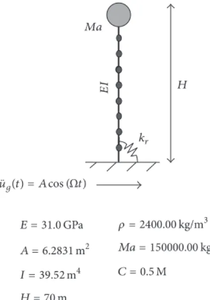
E = 31.0GPa
A = 6.2831m2
I = 39.52m4
H = 70m
휌 = 2400.00kg/m3
Ma = 150000.00kg
C = 0.5M
H
EI
= Acos (Ωt)
̈
ug(t)
Figure 1: Tower model with concentrated mass at top and elastoplastic support.
0 0.05 0.1 0.15 0.2 0.25
Am
p
li
tude no
rm
(m)
Time dom. int.k = 1011kNm/rad
Time dom. int.k =infinite
HBMk = 1011kNm/rad
HBMk =infinite
5.00 10.00 15.00 20.00 25.00 30.00 35.00 40.00
0.00
Ω(rad/s)
Figure 2: Variation of the maximum displacement at the top of the tower as a function of the forcing frequencyΩobtained with the harmonic balance method (HBM) and with time domain integration.𝐴𝑥= 0.8𝑔.
m = 10kg
kl= 5N/m
k = kl+ knlu(t)2
f(t) = 0.4m·cos (휔t)
u(t)
m
Figure 3: 1-DOF model with cubic nonlinear stiffness under harmonic excitation.
whereTis the equivalent rotation matrix, which satisfies the following condition:
T𝑇S(𝜏)𝑇=S(𝜏)𝑇T𝑇. (46)
Taking into account the block-diagonal characteristic ofS(𝜏) and since Tis an orthogonal matrix, it is possible to find
an explicit expression forTas a function ofTthrough the following expression:
T=[[[[
[
t1,1 . . . t1,NGL
... d ...
tNGL,1 . . . tNGL,NGL
]] ]] ]
Time domain simulation Time domain simulation
Proposed method Proposed method
0 5 10 15 20 25 30
Am
p
li
tude no
rm
(m)
0 5 10 15 20 25 30
Am
p
li
tude no
rm
(m)
10 20 30 40
0
Ω(rad/s)
10 20 30 40
0
Ω(rad/s)
kNL= 10N/m3
kNL= −10N/m3
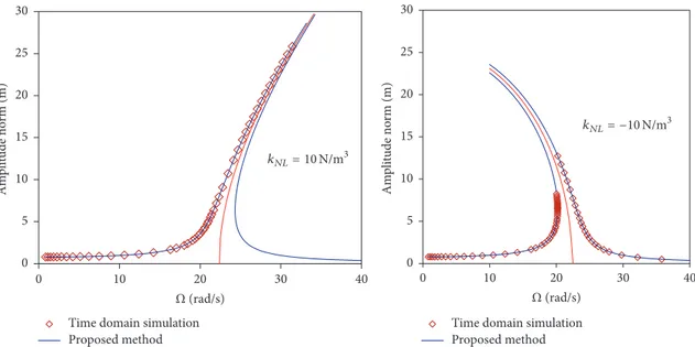
Figure 4: Nonlinear resonance curves. Maximum amplitude as a function of the forcing frequency.
1st mode
2nd mode
3rd mode
4th mode
E = 210GPa
휌 = 7.85ton/m3
d = 15cm
bf = 10cm
Ixx= 6.84e − 12m4
A = 1.73e − 6m2
tw
tf
bf
10.0m
6.0m
y y
d x x H
Figure 5: Pitched-roof frame model and four first natural vibration modes.
where NGL is the number of degrees of freedom andt𝑖,𝑗is a submatrix given by
t𝑖,𝑗=T𝑖,𝑗I3, (48)
whereI3is an identity matrix of order three.
3. Numerical Examples
3.1. Linear Analysis Validation. As a first example, a simple tower model with a concentrated mass at the top and an elastic rotational support at the base is studied to validate the linear formulation. The finite element model is composed of 10 beam-column Euler-Bernoulli elements. The geometrical and material properties are shown in Figure 1. The tower is under the action of a horizontal harmonic base displacement. Figure 2 shows the variation of the maximum displace-ment at the top of the tower as a function of the forcing
frequencyΩ(resonance curve) for a forcing magnitude𝐴𝑥=
0.8𝑔, where𝑔is the acceleration of gravity, considering two values of the elastic support stiffness𝑘𝑟. The results obtained with the present formulation and continuation scheme agree with the results obtained from a time domain analysis. This shows the coherence of the result obtained with the proposed method.
3.2. Nonlinear Analysis Validation. As a second example, a simple mass-spring system with cubic nonlinearity under harmonic excitation is studied to validate the nonlinear formulation. The schematic representation of the system and relevant properties are shown in Figure 3. In this example, damping is not considered.
0 0.005 0.01 0.015 0.02 0.025 0.03 0.035
0.00 50.00 100.00 150.00 200.00
H = 0m
H = 3m
H = 6m
H = 0m
H = 3m
H = 6m Linear
Nonlinear
Linear Nonlinear
Linear Nonlinear
Ω(rad/s)
|D
x
|
50.00 100.00 150.00 200.00
0.00
Ω(rad/s)
50.00 100.00 150.00 200.00
0.00
Ω(rad/s)
Linear Nonlinear
50.00 100.00 150.00 200.00
0.00
Ω(rad/s)
0 0.0005 0.001 0.0015 0.002 0.0025
|D
y
|
Linear Nonlinear
50.00 100.00 150.00 200.00
0.00
Ω(rad/s)
0 0.0005 0.001 0.0015 0.002 0.0025 0.003
|D
y
|
0 0.005 0.01 0.015 0.02 0.025 0.03 0.035
|D
x
|
0 0.005 0.01 0.015 0.02 0.025 0.03 0.035
|D
x
|
Linear Nonlinear
50.00 100.00 150.00 200.00
0.00
Ω(rad/s)
0 0.0005 0.001 0.0015 0.002 0.0025 0.003
|D
y
|
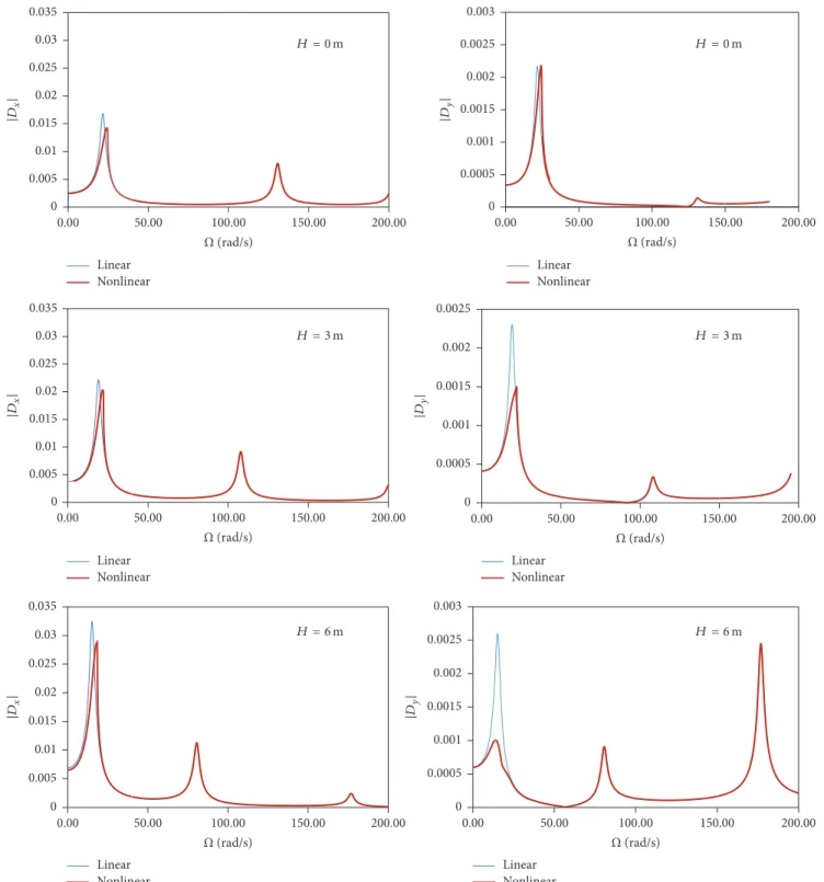
Figure 6: Variation of the norm of the horizontal and vertical vibration amplitudes at the roof top as a function of the excitation frequency for a horizontal base excitation and three values of the roof height𝐻.𝐴𝑥= 0.96𝑔.
obtained with the present HBM-Galerkin scheme and with time domain simulations are very close, validating the non-linear formulation. It can be also observed that the algorithm is able to bypass the limit point associated with the saddle-node bifurcation. As expected, the time domain analysis is not able to trace the unstable branches of resonance curves.
3.3. Frequency Domain Analysis of Slender Frames
H = 6m
H = 3m
Linear Nonlinear
Linear Nonlinear Linear
Nonlinear
H = 0m
50.00 100.00 150.00 200.00
0.00
Ω(rad/s)
50.00 100.00 150.00 200.00
0.00
Ω(rad/s)
50.00 100.00 150.00 200.00
0.00
Ω(rad/s)
0.000 0.005 0.010 0.015 0.020
|D
y
|
0.000 0.005 0.010 0.015 0.020
|D
y
|
0.000 0.005 0.010 0.015 0.020
|D
y
|
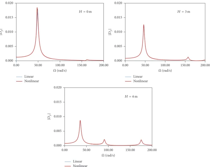
Figure 7: Variation of the norm of the vertical vibration amplitude at the roof top as a function of the excitation frequency for a vertical base excitation and three values of the roof height𝐻.𝐴𝑦= 0.96𝑔.
Table 1: Four first natural frequencies of the pitched-roof frame.
𝐻(m) Natural vibration frequency (rad/s)
1st mode 2nd mode 3rd mode 4th mode
0.0 21.82 48.97 130.54 161
3.0 19.61 47.14 108.23 159.80
6.0 15.40 36.42 83.21 92.08
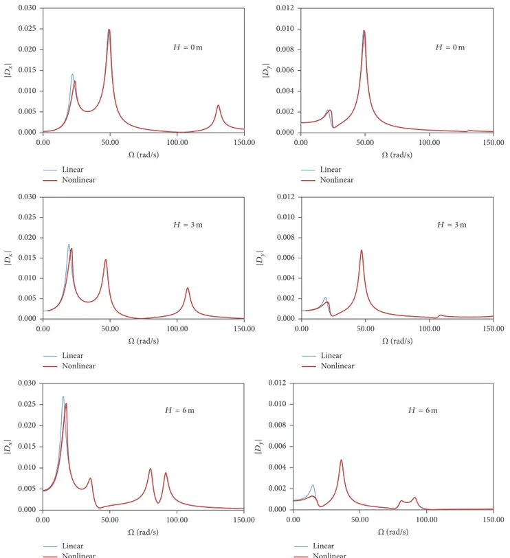
as the configuration of the first four natural vibration modes, with the first and third modes being antisymmetric and the second and fourth modes being symmetric. The influence of the roof height on the response is also investigated. Table 1 shows the first four natural frequencies for the three values of𝐻considered in the numerical analysis. The vibration fre-quencies decrease with𝐻, as the frame slenderness increases. The structure is modeled with twenty bean-column elements: 8 elements of the same size for the columns and 12 elements for the roof.
Figure 6 shows the variation of the norm of the horizontal and vertical components of the displacement at top of the
frame,𝐷𝑥and𝐷𝑦, respectively, as a function of the forcing frequency,Ω, considering both linear (blue) and nonlinear (red) FE formulations for three values of the height of the roof pitches (𝐻 = 0 m, 3 m, and 6 m) and considering a horizontal excitation magnitude:𝐴𝑥= 0.96𝑔. The horizontal base motion excites the first and the third modes only, which correspond to predominantly lateral deformation modes. The nonlinear effect is present in the first resonance region, where a hardening behavior is observed. The first peak and, consequently, the nonlinearity increase with increasing roof height, with the nonlinear maximum vibration amplitude being slightly lower than the linear one. After the first peak, the nonlinear and linear responses are practically coincident. The vertical displacement 𝐷𝑦 is smaller than the vertical component and is overestimated in a linear analysis. Figure 7 displays the response for a vertical excitation magnitude:
𝐴𝑦 = 0.96𝑔. The vertical base motion excites the second
H = 0m
H = 3m
H = 6m
H = 6m Linear
Nonlinear
Linear Nonlinear
Linear Nonlinear Linear
Nonlinear
50.00 100.00 150.00
0.00
Ω(rad/s)
50.00 100.00 150.00
0.00
Ω(rad/s)
50.00 100.00 150.00
0.00
Ω(rad/s)
50.00 100.00 150.00
0.00
Ω(rad/s)
0.000 0.002 0.004 0.006 0.008 0.010 0.012
|D
y
|
H = 3m
Linear Nonlinear
50.00 100.00 150.00
0.00
Ω(rad/s)
0.000 0.002 0.004 0.006 0.008 0.010 0.012
|D
y
|
0.000 0.005 0.010 0.015 0.020 0.025 0.030
|D
x
|
0.000 0.005 0.010 0.015 0.020 0.025 0.030
|D
x
|
H = 0m
Linear Nonlinear
50.00 100.00 150.00
0.00
Ω(rad/s)
0.000 0.002 0.004 0.006 0.008 0.010 0.012
|D
y
|
0.000 0.005 0.010 0.015 0.020 0.025 0.030
|D
x
|
Figure 8: Variation of the norm of the vertical and horizontal vibration amplitudes at the roof top as a function of the excitation frequency for simultaneous vertical and horizontal excitation and three values of the roof height𝐻.𝐴𝑥= 0.8𝑔and𝐴𝑦= 0.667𝐴𝑥.
effect of nonlinearity is negligible. In this case, due to the symmetry of the displacement field, the lateral motion of the top node is zero.
Figure 8 shows the norm of the horizontal and vertical displacement as a function of the forcing frequency for the frame excited in both the horizontal and vertical directions.
1st mode
2nd mode
3rd mode
4th mode
E = 210GPa
휌 = 7.85ton/m3
d = 15cm
bf = 10cm
Ixx= 6.84e − 12m4
A = 1.73e − 6m2
tw
tf
bf
10.0m
6.0m
y y
d x x
H R = 10
sin (2 arctg(H/10))
Figure 9: Arched-roof frame model and four first natural vibration modes.
H = 1m H = 3m
H = 5m Linear Nonlinear Linear
Nonlinear
Linear Nonlinear
0.000 0.005 0.010 0.015 0.020 0.025 0.030
|D
x
|
0.000 0.005 0.010 0.015 0.020 0.025 0.030
|D
x
|
0.000 0.005 0.010 0.015 0.020 0.025 0.030
|D
x
|
50.00 100.00 150.00 200.00
0.00
Ω(rad/s)
50.00 100.00 150.00 200.00
0.00
Ω(rad/s)
50.00 100.00 150.00 200.00
0.00
Ω(rad/s)
Figure 10: Influence of the roof height on the nonlinear response of the arched-roof frame under horizontal excitation.𝐴𝑥= 0.96𝑔.
evident in the two first resonance regions, where a hardening behavior, leading to possible dynamic jumps, is observed. As the roof height increases, the magnitude of𝐷𝑥corresponding to the first resonant peak increases, while the magnitude of second peak decreases. On the other hand, the magnitude
0.000 0.005 0.010 0.015 0.020
|D
y
|
H = 1m H = 3m
H = 5m Linear Nonlinear
Linear Nonlinear Linear
Nonlinear
50.00 100.00 150.00 200.00
0.00
Ω(rad/s)
50.00 100.00 150.00 200.00
0.00
Ω(rad/s)
0.000 0.005 0.010 0.015 0.020
|D
y
|
50.00 100.00 150.00 200.00
0.00
Ω(rad/s)
0.000 0.005 0.010 0.015 0.020
|D
y
|
Figure 11: Influence of the roof height on the nonlinear response of the arched-roof frame under vertical excitation.𝐴𝑦= 0.96𝑔.
continuation techniques. The solutions between the two limit points are unstable.
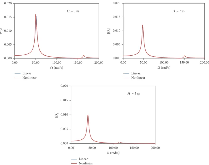
3.3.2. Arched-Roof Frame. Now, an arched-roof frame fixed at the base and with a constant cross section is studied to assess the behavior of this typical structural form under horizontal and vertical base excitation. The structure has the same span, column height, and cross section as the pitched roof, as well as the same material properties, as shown in Figure 9, to enable comparisons of the results. An incomplete circular arch with height 𝐻is considered. Figure 9 also shows the configuration of the first four vibration modes. Table 2 shows the first four natural frequencies for three values of the arch height, 𝐻. As in the previous example, the first and third modes are antisymmetric, while the second and fourth modes are symmetric.
Figures 10 and 11 show the variation of the norm of the vertical and horizontal displacements at top of the arch as a function of the forcing frequency for horizontal and vertical harmonic excitation, respectively, and considering both linear (blue) and nonlinear (red) formulations. For the
Table 2: Natural vibration frequencies of the arched-roof frame.
𝐻(m) Natural vibration frequency (rad/s)
1st mode 2nd mode 3rd mode 4th mode
1.0 21.02 51.73 122.60 167.05
3.0 17.81 48.51 97.77 151.60
5.0 13.20 40.79 74.02 113.41
H = 1m H = 1m
H = 3m
H = 3m
H = 5m H = 5m
Linear Nonlinear
Linear Nonlinear
Linear Nonlinear
Linear Nonlinear
Linear Nonlinear
Linear Nonlinear
50.00 100.00 150.00
0.00
Ω(rad/s)
50.00 100.00 150.00
0.00
Ω(rad/s)
50.00 100.00 150.00
0.00
휔(rad/s)
50.00 100.00 150.00
0.00
Ω(rad/s)
50.00 100.00 150.00
0.00
Ω(rad/s)
50.00 100.00 150.00
0.00
Ω(rad/s)
0.000 0.005 0.010 0.015 0.020 0.025
|D
x
|
0.000 0.005 0.010 0.015 0.020 0.025 0.030
|D
x
|
0.000 0.005 0.010 0.015 0.020 0.025
|D
x
|
0.000 0.002 0.004 0.006 0.008 0.010
|D
y
|
0.000 0.002 0.004 0.006 0.008 0.010
|D
y
|
0.000 0.002 0.004 0.006 0.008 0.010
|D
y
|
Figure 12: Variation of the norm of the vertical and horizontal vibration amplitudes at the roof top as a function of the excitation frequency for simultaneous vertical and horizontal excitation and three values of the roof height𝐻.𝐴𝑥= 0.8𝑔and𝐴𝑦= 0.667𝐴𝑥.
Figure 12 shows the variation of the maximum horizontal (𝐷𝑥) and vertical displacements (𝐷𝑦) at the top of arch, considering both horizontal and vertical base excitations with
𝐴𝑦 = 0.667𝐴𝑥 and 𝐴𝑥 = 0.8𝑔. In this case, all vibration
modes are excited. The influence of the geometric nonlin-earity is evident in the two first resonance regions, where
a hardening behavior leading to possible dynamic jumps is observed. As the roof height increases, the magnitude of
𝐷𝑥corresponding to the first resonant peak increases, while
0.000 0.010 0.020 0.030 0.040 0.050 0.060
|D
x
|
0.000 0.010 0.020 0.030 0.040 0.050 0.060
|D
x
|
0.000 0.010 0.020 0.030 0.040 0.050 0.060
|D
x
|
20.00 40.00 60.00 80.00 100.00
0.00
Ω(rad/s)
20.00 40.00 60.00 80.00 100.00
0.00
Ω(rad/s)
20.00 40.00 60.00 80.00 100.00
0.00
Ω(rad/s)
20.00 40.00 60.00 80.00 100.00
0.00
Ω(rad/s)
20.00 40.00 60.00 80.00 100.00
0.00
Ω(rad/s)
20.00 40.00 60.00 80.00 100.00
0.00
Ω(rad/s)
0.000 0.003 0.006 0.009 0.012 0.015 0.018
|D
y
|
0.000 0.003 0.006 0.009 0.012 0.015 0.018
|D
y
|
0.000 0.003 0.006 0.009 0.012 0.015 0.018
|D
y
|
H = 0m
H = 0m
H = 3m H = 3m
H = 6m
H = 6m Linear
Nonlinear
Linear Nonlinear
Linear Nonlinear
Linear Nonlinear
Linear Nonlinear
Linear Nonlinear
Figure 13: Influence of the roof height on the nonlinear response of the frame under horizontal and vertical excitation.𝐴𝑥= 0.8𝑔and𝐴𝑦=
0.667𝐴𝑥.
3.3.3. Pitched-Roof Frame with a Long Span. Now, the pitched roof is again analyzed considering a span length𝐿 = 16.0m, increasing thus the frame’s slenderness. The other properties of the system are the same as those shown in Figure 5. Table 3 shows the first four natural frequencies for the three values of
the roof height. Compared with the results in Table 1, a strong decrease in the natural frequencies is observed.
Linear Nonlinear
Linear Nonlinear
Linear Nonlinear
Linear Nonlinear
Ax= 0.48g Ax= 0.96g
Ax= 1.8g
Ax= 3.6g 0
0.005 0.01 0.015 0.02 0.025 0.03 0.035
|D
x
|
20.00 40.00 60.00 80.00 100.00
0.00
Ω(rad/s)
20.00 40.00 60.00 80.00 100.00
0.00
Ω(rad/s)
20.00 40.00 60.00 80.00 100.00
0.00
Ω(rad/s)
0 0.02 0.04 0.06 0.08 0.1 0.12 0.14
|D
x
|
0 0.01 0.02 0.03 0.04 0.05 0.06 0.07
|D
x
|
0 0.002 0.004 0.006 0.008 0.01 0.012 0.014 0.016 0.018
|D
x
|
20.00 40.00 60.00 80.00 100.00
0.00
Ω(rad/s)
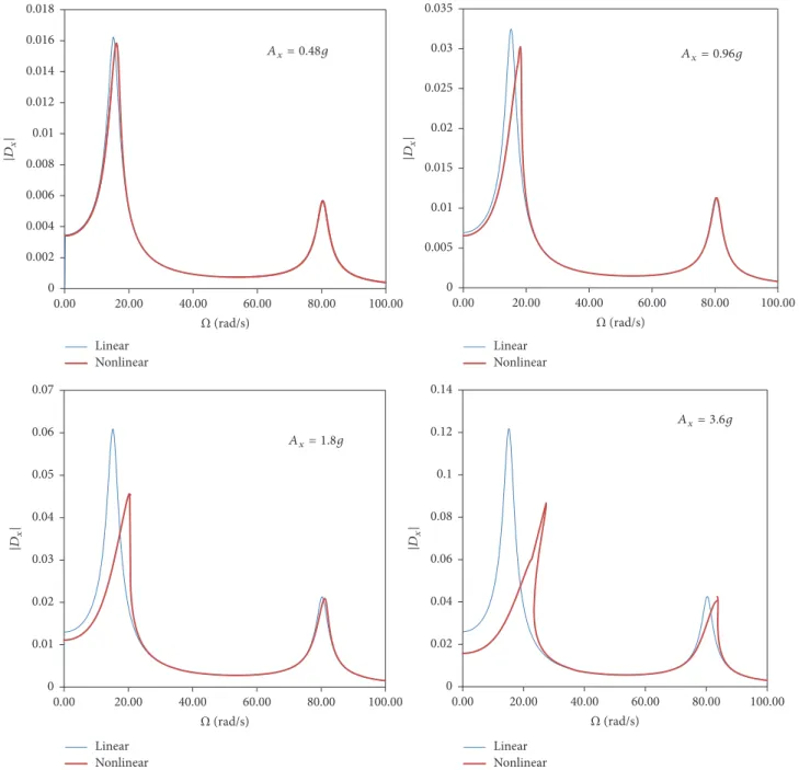
Figure 14: Influence of increasing magnitude𝐴𝑥on the nonlinear response of the frame under horizontal excitation. Norm of the horizontal displacement at top of pitched-roof as a function of the forcing frequency.𝐿 = 10and𝐻 = 6m.
acting simultaneously with amplitude of the horizontal accel-eration of 𝐴𝑥 = 0.8𝑔and vertical acceleration of 𝐴𝑦 =
0.66𝐴𝑥. The nonlinear effects are visible in the two first
resonance regions, similar to the frame with 𝐿 = 10m. However, the two first natural frequencies are close, especially
for 𝐻 = 0m, leading to modal interaction between the
two first modes and a large excitation region, where large-amplitude vibrations occur. Compared with the results in Figure 6, for𝐿 = 10m, a marked increase in the lateral and vertical displacements is observed. The vertical displace-ments are particularly large around the second vibration frequency.
3.3.4. Strong Base Motion. Now, the effect of strong base motion on the nonlinear dynamics of the pitched-roof frame (Section 3.3.1), arched-roof (Section 3.3.2) frame, and pitched-roof frame with long span (Section 3.3.3) is assessed. For this, a parametric study considering the variation of the ground acceleration magnitude is presented. A maximum acceleration peak of 3.6𝑔 for a single direction excitation and of 3.0𝑔 for horizontal and vertical excitations acting simultaneously is adopted.
Linear Nonlinear
Linear Nonlinear
Ay= 1.8g
Ay= 3.6g
20.00 40.00 60.00 80.00 100.00
0.00
Ω(rad/s)
20.00 40.00 60.00 80.00 100.00
0.00
Ω(rad/s)
0 0.005 0.01 0.015 0.02 0.025 0.03 0.035 0.04 0.045
|D
y
|
0 0.002 0.004 0.006 0.008 0.01 0.012 0.014 0.016 0.018
|D
y
|
Figure 15: Influence of increasing base motion𝐴𝑥on the nonlinear response of the frame under vertical excitation. Norm of the vertical displacement at top of pitched roof as a function of the forcing frequency.𝐿 = 10m and𝐻 = 6m.
Table 3: Natural vibration frequency of pitched-roof frame.
𝐻(m) Natural frequency of vibration (rad/s) 1st mode 2nd mode 3rd mode 4th mode
0.0 16.60 21.09 60.68 117.35
3.0 15.52 25.58 58.03 91.95
6.0 12.93 24.82 50.24 59.47
excitation magnitude. A sharp increase in the vibration amplitude and the hardening nonlinearity of the response in the first resonance region is observed. For strong base motions, the effect of the nonlinearity in the vicinity of the third vibration frequency begins to appear, being also of the hardening type. The second mode is not excited.
Figure 15 shows the frame response due to vertical harmonic acceleration, considering𝐴𝑥 = 1.8𝑔and 𝐴𝑥 =
3.6𝑔. The effect of the geometric nonlinearity is observed in the resonance regions associated with the second and fourth vibration modes, exhibiting softening behavior. The softening behavior is due to quadratic nonlinearities and is connected with the interaction between axial and transver-sal beam displacements. In such cases, the linear analy-sis underestimates the maximum vibration response. The softening effect due to negative quadratic nonlinearity can be observed in other slender structures under compres-sive loads like shallow arches and arises from the inter-action between in-plane compressive forces and bending [25].
Figure 16 shows the horizontal and vertical components of vibration as function of forcing frequency at top of
pitched-roof frame (𝐿 = 10m and𝐻 = 6m), considering harmonic horizontal and vertical base excitations acting simultaneously and considering 𝐴𝑦 = 0.667𝐴𝑥 and two values of the acceleration amplitude:𝐴𝑥 = 1.5𝑔and𝐴𝑥 =
3.0𝑔. The nonlinear effect is present in all resonance regions for the two displacement components. A strong difference between the linear and nonlinear responses is particularly observed in the first resonance region.
Finally, Figure 17 shows the horizontal and vertical displacement components at top of pitched-roof frame as a function of forcing frequency for the frame with𝐿 = 16m
and𝐻 = 6m, considering harmonic horizontal and vertical
base excitations acting simultaneously with𝐴𝑦 = 0.667𝐴𝑥, for two values of𝐴𝑥:1.5𝑔and3.0𝑔. Again, the strong base motion leads to a highly nonlinear response.
In all cases analyzed here, the resonance curves for the lin-ear and nonlinlin-ear cases were easily obtained by the proposed numerical methodology, which can be easily applied to any structural system discretized by the FEM.
4. Conclusions
Linear Nonlinear
Linear Nonlinear
Linear Nonlinear
Linear Nonlinear
Ax= 1.5g
Ay= 1.0g
Ax= 3.0g
Ay= 2.0g
Ax= 1.5g
Ay= 1.0g
Ax= 3.0g
Ay= 2.0g
20.00 40.00 60.00 80.00 100.00
0.00
Ω(rad/s)
20.00 40.00 60.00 80.00 100.00
0.00
Ω(rad/s)
20.00 40.00 60.00 80.00 100.00
0.00
Ω(rad/s)
20.00 40.00 60.00 80.00 100.00
0.00
Ω(rad/s)
0 0.001 0.002 0.003 0.004 0.005 0.006 0.007 0.008 0.009 0.01
|D
y
|
0 0.01 0.02 0.03 0.04 0.05 0.06
|D
x
|
0 0.02 0.04 0.06 0.08 0.1 0.12
|D
x
|
0 0.002 0.004 0.006 0.008 0.01 0.012 0.014 0.016 0.018 0.02
|D
y
|
Figure 16: Horizontal and vertical displacements at top of the frame as a function of the forcing frequency due to simultaneous horizontal and vertical forcing.𝐿 = 10m and𝐻 = 6m.
of the modal amplitudes and forcing frequency is solved by the Newton-Raphson method together with an arc-length procedure to obtain the nonlinear resonance curves. The formulation of the proposed method is validated comparing the present results with time domain simulations showing coherence and precision. The algorithm is able to map regions with coexisting stable and unstable solutions. A pitched-roof frame and an arched-pitched-roof frame under horizontal and vertical base excitation with varying roof height and spans are studied to illustrate the influence of the nonlinearity on the four first resonance regions. Horizontal base motion
Linear Nonlinear
Linear Nonlinear
Linear Nonlinear
Linear Nonlinear 0.000
0.050 0.100 0.150 0.200 0.250 0.000 0.020 0.040 0.060 0.080 0.100 0.120
20.00 40.00 60.00 80.00 100.00
0.00
Ω(rad/s)
20.00 40.00 60.00 80.00 100.00
0.00
Ω(rad/s)
20.00 40.00 60.00 80.00 100.00
0.00
Ω(rad/s)
20.00 40.00 60.00 80.00 100.00
0.00
Ω(rad/s)
|D
x
|
|D
x
|
Ax= 3.0g
Ay= 2.0g
Ax= 1.5g
Ay= 1.0g
Ax= 1.5g
Ay= 1.0g
Ax= 3.0g
Ay= 2.0g 0.000
0.002 0.004 0.006 0.008 0.010 0.012 0.014 0.016 0.018
|D
y
|
0.000 0.005 0.010 0.015 0.020 0.025 0.030 0.035
|D
y
|
Figure 17: Horizontal and vertical displacements at the top of the frame as a function of the forcing frequency due to simultaneous horizontal and vertical forcing.𝐿 = 16m and𝐻 = 6m.
can be used as a preliminary design tool for frames under seismic and other types of base excitation, leading to a safer design.
Conflicts of Interest
The authors declare that there are no conflicts of interest regarding the publication of this paper.
References
[1] W. T. Koiter, “Post-buckling analysis of simple two-bar frame,” inRecent Progress in Applied Mechanics, B. Broberg, J. Hult, and F. Niordson, Eds., pp. 337–354, 1967.
[2] J. Roorda,The instability of imperfect elastic structures [Ph.D. thesis], University College London, London, UK, 1965. [3] Z. Bazant and L. Cedolin,Stability of Structures, Oxford
Univer-sity Press, Oxford, UK, 1991.
[4] T. V. Galambos, Guide to Stability Design Criteria for Metal Structures, John Wiley & Sons, 1998.
[5] N. Silvestre and D. Camotim, “Asymptotic-numerical method to analyze the postbuckling behavior, imperfection-sensitivity, and mode interaction in frames,” Journal of Engineering Mechanics, vol. 131, no. 6, pp. 617–632, 2005.
[7] A. S. Galv˜ao, P. B. Gonc¸alves, and R. A. M. Silveira, “Post-buckling behavior and imperfection sensitivity of L-frames,” International Journal of Structural Stability and Dynamics, vol. 5, no. 1, pp. 19–35, 2005.
[8] G. J. Simitses, “Effect of static preloading on the dynamic stability of structures,”AIAA journal, vol. 21, no. 8, pp. 1174–1180, 1983.
[9] S. L. Chan and G. W. M. Ho, “Nonlinear vibration analysis of steel frames with semirigid connections,”Journal of Structural Engineering, vol. 120, no. 4, pp. 1075–1087, 1994.
[10] C. E. N. Mazzilli and R. M. L. R. F. Brasil, “Effect of static loading on the nonlinear vibrations of a three-time redundant portal frame: analytical and numerical studies,”Nonlinear Dynamics, vol. 8, no. 3, pp. 347–366, 1995.
[11] M. E. S. Soares and C. E. N. Mazzilli, “Nonlinear normal modes of planar frames discretized by the finite element method,” Computers and Structures, vol. 77, no. 5, pp. 485–493, 2000. [12] S. L. Chan and P. T. Chui, Eds.,Non-Linear Static and Cyclic
Analysis of Steel Frames with Semi-Rigid Connections, Elsevier, 2000.
[13] M. I. McEwan, J. R. Wright, J. E. Cooper, and A. Y. T. Leung, “A combined modal/finite element analysis technique for the dynamic response of a non-linear beam to harmonic excitation,” Journal of Sound and Vibration, vol. 243, no. 4, pp. 601–624, 2001.
[14] P. Ribeiro, “Hierarchical finite element analyses of geometrically non-linear vibration of beams and plane frames,” Journal of Sound and Vibration, vol. 246, no. 2, pp. 225–244, 2001. [15] J. G. S. Da Silva, L. R. O. De Lima, P. D. S. Vellasco, S. De
Andrade, and R. A. De Castro, “Nonlinear dynamic analysis of steel portal frames with semi-rigid connections,”Engineering Structures, vol. 30, no. 9, pp. 2566–2579, 2008.
[16] A. S. Galv˜ao, A. R. D. Silva, R. A. M. Silveira, and P. B. Gonc¸alves, “Nonlinear dynamic behavior and instability of slender frames with semi-rigid connections,”International Journal of Mechan-ical Sciences, vol. 52, no. 12, pp. 1547–1562, 2010.
[17] W. Su and C. E. S. Cesnik, “Strain-based geometrically non-linear beam formulation for modeling very flexible aircraft,” International Journal of Solids and Structures, vol. 48, no. 16-17, pp. 2349–2360, 2011.
[18] P. B. Gonc¸alves, D. L. B. R. Jurjo, C. Magluta, and N. Roitman, “Experimental investigation of the large amplitude vibrations of a thin-walled column under self-weight,”Structural Engineering and Mechanics, vol. 46, no. 6, pp. 869–886, 2013.
[19] A. R. Masoodi and S. H. Moghaddam, “Nonlinear dynamic analysis and natural frequencies of gabled frame having flexible restraints and connections,”KSCE Journal of Civil Engineering, vol. 19, no. 6, pp. 1819–1824, 2015.
[20] J. L. Palacios Felix, J. M. Balthazar, and R. M. L. R. F. Brasil, “On saturation control of a non-ideal vibrating portal frame founda-tion type shear-building,”Journal of Vibration and Control, vol. 11, no. 1, pp. 121–136, 2005.
[21] T. S. Parker and L. O. Chua,Practical Numerical Algorithms for Chaotic Systems, Springer, New York, NY, USA, 1989.
[22] M. S. Nakhla and J. Vlach, “A piecewise harmonic balance technique for determination of periodic response of nonlinear systems,”IEEE Transactions on Circuits and Systems, vol. 23, no. 2, pp. 85–91, 1976.
[23] S. L. Lau, Y. K. Cheung, and S. Y. Wu, “Incremental harmonic balance method with multiple time scales for aperiodic vibra-tion of nonlinear systems,”ASME Journal of Applied Mechanics, vol. 50, no. 4, pp. 871–876, 1983.
[24] Y. K. Cheung and S. H. Chen, “Application of the incremental harmonic balance method to cubic non-linearity systems,” Journal of Sound and Vibration, vol. 140, no. 2, pp. 273–286, 1990.
[25] S. H. Chen, Y. K. Cheung, and H. X. Xing, “Nonlinear vibration of plane structures by finite element and incremental harmonic balance method,”Nonlinear Dynamics, vol. 26, no. 1, pp. 87–104, 2001.
[26] A. Grolet and F. Thouverez, “Computing multiple periodic solutions of nonlinear vibration problems using the harmonic balance method and Groebner bases,”Mechanical Systems and Signal Processing, vol. 52-53, no. 1, pp. 529–547, 2015.
[27] P. Ribeiro and M. Petyt, “Geometrical non-linear, steady state, forced, periodic vibration of plates, part I: model and conver-gence studies,”Journal of Sound and Vibration, vol. 226, no. 5, pp. 955–983, 1999.
[28] G. Von Groll and D. J. Ewins, “The harmonic balance method with arc-length continuation in rotor/stator contact problems,” Journal of Sound and Vibration, vol. 241, no. 2, pp. 223–233, 2001. [29] J. V. Ferreira and A. L. Serpa, “Application of the arc-length method in nonlinear frequency response,”Journal of Sound and Vibration, vol. 284, no. 1-2, pp. 133–149, 2005.
[30] J. M. Londo˜no, S. A. Neild, and J. E. Cooper, “Identification of backbone curves of nonlinear systems from resonance decay responses,”Journal of Sound and Vibration, vol. 348, pp. 224– 238, 2015.
[31] L. Renson, G. Kerschen, and B. Cochelin, “Numerical compu-tation of nonlinear normal modes in mechanical engineering,” Journal of Sound and Vibration, vol. 364, pp. 177–206, 2016. [32] S. Stoykov and P. Ribeiro, “Nonlinear free vibrations of beams
in space due to internal resonance,” Journal of Sound and Vibration, vol. 330, no. 18-19, pp. 4574–4595, 2011.
[33] S. Stoykov and P. Ribeiro, “Stability of nonlinear periodic vibrations of 3D beams,”Nonlinear Dynamics, vol. 66, no. 3, pp. 335–353, 2011.
[34] G. Formica, A. Arena, W. Lacarbonara, and H. Dankowicz, “Coupling FEM with parameter continuation for analysis of bifurcations of periodic responses in nonlinear structures,” Journal of Computational and Nonlinear Dynamics, vol. 8, no. 2, Article ID 021013, 2013.
[35] L. F. Paullo Mu˜noz, P. B. Gonc¸alves, R. A. M. Silveira, and A. R. D. Silva, “Non-linear dynamic analysis of plane frame structures under seismic load in frequency domain,” inProceedings of the International Conference on Engineering Vibration, Ljubljana, Slovenia, September 2016.
[36] https://en.wikipedia.org/wiki/Peak ground acceleration. [37] J. Douglas, “Earthquake ground motion estimation using
strong-motion records: a review of equations for the estimation of peak ground acceleration and response spectral ordinates,” Earth-Science Reviews, vol. 61, no. 1, pp. 43–104, 2003. [38] E. I. Katsanos, A. G. Sextos, and G. D. Manolis, “Selection of
earthquake ground motion records: a state-of-the-art review from a structural engineering perspective,”Soil Dynamics and Earthquake Engineering, vol. 30, no. 4, pp. 157–169, 2010. [39] A. H. Nayfeh and D. T. Mook,Nonlinear Oscillations, John Wiley
& Sons, 2008.
[40] R. Bouc, “Sur la m´ethode de Galerkin-Urabe pour les syst`emes diff´erentiels p´eriodiques,”International Journal of Non-Linear Mechanics, vol. 7, no. 2, pp. 175–188, 1972.
[42] E. Ramm, “Strategies for tracing the non-linear response near limit-points,” inNonlinear Finite Element Analysis in Structural Mechanics, W. Wunderlich, E. Stein, and K. J. Bathe, Eds., pp. 63–89, Springer, Berlin, Germany, 1981.
,QWHUQDWLRQDO-RXUQDORI
$HURVSDFH
(QJLQHHULQJ
+LQGDZL3XEOLVKLQJ&RUSRUDWLRQKWWSZZZKLQGDZLFRP 9ROXPH
Robotics
Journal ofHindawi Publishing Corporation
http://www.hindawi.com Volume 2014
Hindawi Publishing Corporation
http://www.hindawi.com Volume 2014
Active and Passive Electronic Components
Control Science and Engineering
Journal of
Hindawi Publishing Corporation
http://www.hindawi.com Volume 2014
Machinery
Hindawi Publishing Corporation
http://www.hindawi.com Volume 2014
Hindawi Publishing Corporation http://www.hindawi.com
Journal of
(QJLQHHULQJ
Volume 201Submit your manuscripts at
https://www.hindawi.com
VLSI Design
Hindawi Publishing Corporation
http://www.hindawi.com Volume 201
-Hindawi Publishing Corporation
http://www.hindawi.com Volume 2014
Shock and Vibration
Hindawi Publishing Corporation
http://www.hindawi.com Volume 2014
Civil Engineering
Advances inAcoustics and VibrationAdvances in Hindawi Publishing Corporation
http://www.hindawi.com Volume 2014
Hindawi Publishing Corporation
http://www.hindawi.com Volume 2014
Electrical and Computer Engineering
Journal of
Advances in OptoElectronics
Hindawi Publishing Corporation
http://www.hindawi.com Volume 2014
The Scientific
World Journal
Hindawi Publishing Corporation
http://www.hindawi.com Volume 2014
Sensors
Journal ofHindawi Publishing Corporation
http://www.hindawi.com Volume 2014
Modelling & Simulation in Engineering
Hindawi Publishing Corporation
http://www.hindawi.com Volume 2014
Hindawi Publishing Corporation
http://www.hindawi.com Volume 2014
Chemical Engineering
International Journal of Antennas and Propagation
International Journal of
Hindawi Publishing Corporation
http://www.hindawi.com Volume 2014
Hindawi Publishing Corporation
http://www.hindawi.com Volume 2014
Navigation and Observation
International Journal of
Hindawi Publishing Corporation
http://www.hindawi.com Volume 2014