ABSTRACT: The present paper focuses on the effect of swirl on important parameters of conical diffusers lows such as static pressure evolution, recirculation zones and wall shear stress. Governing equations are solved using a software based on the inite volume method. Moreover, turbulence effects are taken into account employing the k-ε RNG model with an ennhaced wall treatment. The Reynolds number has been kept constant at 105, and various diffuser geometries were simulated, maintaining a high area ratio of 7 and varying the total divergence angle (16°, 24°, 40°, and 60°). Results showed that the swirl velocity component develops into a Rankine-vortex type or a forced-vortex type. In the former, swirl is not effective to prevent boundary layer separation, and a tailpipe is recommended to allow a large-scale mixing to enhance the pressure recovery process. In the latter case, boundary layer separation is prevented but an intermediary recirculation zone appears. Higher pressure recovery is attained at the exit of the diffuser with swirl addition, without the need of a tailpipe. Results also suggest that there is exists an imposed swirl intensity where the energy losses are minimum thus leading pressure recovery to an optimum level.
KEYWORDS: Static pressure recovery, Wide-angle diffuser, Swirl intensity, Radial pressure gradient, Intermediary recirculation zone.
Numerical Analysis of Swirl Effects on
Conical Diffuser Flows
Eron Tiago Viana Dauricio1, Claudia Regina de Andrade1
INTRODUCTION
Difusers are widely used in many industrial devices and applications in order to convert kinetic energy into static pressure. Examples include applications in gas turbines, water turbines drat tubes, piping systems, and more. In real lows, however, this conversion process is taken at the cost of total energy, which decreases because of dissipative mechanisms, and the aim is always to design a difuser with the best possible eiciency.
For uniform or fully developed inlet lows, the changes in performance of difusers due to geometry are well known and these data are generally written in chart form to simplify the design process, where a coeicient of performance is plotted against area and/or length (L) ratio of the difuser (ESDU 1990). However, in practical situations, because of physical constraints, one cannot always design and build a difuser with optimum performance according to its geometry (i.e. area ratio or length constraint), and generally the difuser will have angles wider than the optimum. his may cause a rapid growth in boundary layer because of the strong pressure gradient, and the boundary layer may separate creating a recirculating region, decreasing the efective low area and increasing the energy losses. herefore, ways of achieving improved diffuser performance under non-optimum geometries must be accomplished. Various methods for improving performance have been proposed and attempted, such as application of suction, injection of a secondary low, introduction of vanes to divide the difuser into several smaller angle difusers, or the introduction of vortex and rotational low at the inlet. he latter is of particular importance because it is present in many industrial lows; therefore, the capacity to predict and understand the physical phenomenon behind this type of low is of paramount importance.
1.Departamento de Ciência e Tecnologia Aeroespacial – Instituto Tecnológico de Aeronáutica – Divisão de Aeronáutica – São José dos Campos/SP – Brazil
Author for correspondence: Claudia Regina de Andrade | Departamento de Ciência e Tecnologia Aeroespacial – Instituto Tecnológico de Aeronáutica – Divisão de Aeronáutica | Praça Marechal do Ar Eduardo Gomes, 50 – Vila das Acácias | CEP: 12.228-900 – São José dos Campos/SP – Brazil | Email: [email protected]
h e addition of swirl to the l ow induces radial pressure gradients and centrifugal forces that push the l uid towards the dif user wall, preventing the excessive growth of the boundary layer and counteracting the tendency of l ow separation, thus increasing the dif user ei ciency and performance. However, the addition of swirl also decreases the axial momentum near the centerline, which is expected from the analysis of mass conservation; depending on the swirl intensity, there may appear a central recirculating zone. h e phenomenon giving rise to this central recirculating zone is called vortex breakdown.
Extensive theoretical and experimental studies and reviews on vortex stability and breakdown have been carried out in the past by Leibovich (1984), Faler and Leibovich (1977), Escudier (1988), Escudier and Keller (1985), Sloan et al. (1986) and Chen et al. (1997), generally in straight tube geometries. Sarpkaya (1974) performed experiments and studies on this theme in diverging tube geometries, which accounts for the inl uence of pressure gradient in the phenomenon. As of swirl addition to the l ow for performance improvement in conical dif users, many experimental studies have been carried out, for example, Neve and Wirasinghe (1978), Senoo et al. (1978), Okhio etal. (1983) and McDonald et al. (1971), in which they all mention the appearance of a central recirculating zone depending on the swirl intensity. Numerical studies have also been developed to predict swirling l ows, such as the predictions of Cho and Fletcher (1989), Armi eld et al. (1990), Okhio et al. (1986) and Pordal et al. (1993). Nonetheless, the experimental studies that have been carried out so far focus mostly on the performance analysis and improvement, using pressure recovery coei cient and ei ciency parameters. h erefore vortex breakdown phenomenon is actually avoided instead of discussed. h e present study aims at the analysis of the ef ect of swirl addition to the conical dif user l ow pattern, including the regime when vortex breakdown occurs and its relation to static pressure evolution, boundary layer separation and radial pressure gradient. Present results also allow to identify the relationship between swirl velocity proi le and dif user wall slope.
MATERIAL AND METHODS
GOVERNING EQUATIONS
Governing equations (cylindrical coordinates) for an incompressible axisymmetric steady turbulent l ow can be given as:
where: –vr , –vθ and –vx are the mean components of the velocity in the radial, tangential and axial direction, respectively; τ –ij is the symmetric viscous stress tensor; τ –R
ij = vivj represent the
Reynolds-stress tensor; fi are the components of external forces, which are zero in this case.
For the axisymmetric l ow considered, the viscous stress tensor components are given by:
(1)
(2)
(3)
(4)
where: v = μ/ρ.
h ese equations can be easily derived from the conservation form of the Navier-Stokes equations using the proper operations for the V operator in cylindrical coordinates (see, for example, Bird et al. 2002).
(5)
TURBULENCE MODELING
Because of the Reynolds-averaging process and the consequent appearance of the Reynolds-stress tensor, we now have 4 equations and 10 unknowns (i.e. pressure, 3 velocity components and the 6 components of the Reynolds-stress tensor), and thus a closure problem. To overcome the closure problem, we need to correlate the Reynolds-stress tensor components to known quantities. h e turbulence model used in this study lies under the eddy-viscosity turbulence model category, which makes use of the Boussinesq hypothesis and is called the k-ε RNG model (Yakhot and Orszag 1986), derived using a statistical technique called renormalization group. It was used with a modii cation to account for swirling l ows, as described in Galván et al. (2011). As shown by the research of Escue and Cui (2010), the k-ε RNG model yields good results for the prediction of mean velocity components under low-to-moderate swirl numbers.
SWIRL NUMBER
Swirling l ows are characterized by a tangential velocity component in addition to the axial velocity component of swirl-free l ows. h is can be accomplished in a number of ways, for example, passing the flow radially through blades and controlling the amount of swirl addition by changing the angle of the blades, or passing the l ow through a rotating honeycomb device. Dif erent types of swirl addition may create dif erent characteristics on the swirling l ow. h ere may exist a Rankine-vortex type, where a core region of the l ow is dominated by viscous ef ects and a forced-vortex type is present as well as an outer region consisting of a free-vortex type. h ere may exist a full forced-vortex type (solid-body rotation) where the tangential velocity linearly increases with radius (Najai et al. 2011). In this paper, we use the dei nition of swirl number, S, as being the ratio between the tangential momentum l ux and the axial momentum l ux, as given by Rocklage-Marliani et al. (2003):
coupling. Both the convection and diffusion terms were discretized using a 2nd-order upwind scheme. All simulations were carried out until the maximum residuals of all variables reached a value of 10−5.
Dif erent geometries of conical dif users were tested with an area ratio equal to 7 and varying total angles of 16°; 24°; 40°; and 60°. Meshes for each geometry were generated using 45 divisions in the radial direction, while the divisions in the axial one ranged from 150 to 300, depending on the dif user length, which is a function of the total angle of divergence. It is worth mentioning that it is important for the grid to be relatively i ne in the axial direction because of the swirl decay, which also needs to be predicted in order to accomplish accurate results. h e y+ value was within the recommended range for the turbulence model currently used (Bigarella and Azevedo 2006).
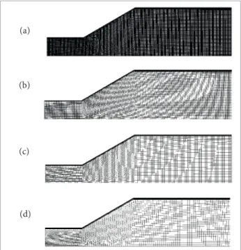
Near-Cartesian meshes were employed, with average orthogonal quality of about 0.99 and average skewness less than 0.2. Skewness is most af ected in the divergence region of the dif user geometry. A grid rei nement study was performed in terms of the grid size, using the 60°-dif user. Four meshes were tested, which are shown in Fig. 1. h e basic properties of each mesh are summarized in Table 1. As the problem is axisymmetric, only half dif user needs to be drawn and numerically solved.
An incompressible l ow with inlet swirl number of 0.3 was simulated for this grid sensitivity analysis. Swirl decay throughout
(7)
(a)
(b)
(c)
(d) NUMERICAL PROCEDURE
Dif user turbulent l ow was simulated using the sot ware ANSYS 16.1, a i nite volume-based solver employing the k-ε RNG model with an adaption for swirl-dominated l ows. h e SIMPLE algorithm was used as a strategy for the velocity-pressure
Table 2. Maximum difference of the four tested grids relative to each other.
Grid #1 Grid #2 Grid #3 Grid #4
Grid #1 - 1.39% 1.22% 6.1%
Grid #2 1.39% - 0.98% 5.76%
Grid #3 1.22% 0.98% - 5.63%
Grid #4 6.1% 5.76% 5.63%
-the difuser can be analyzed, as -the number of axial divisions also varies for each mesh.
Swirl number across sections inside the difuser domain was calculated according to Eq. 7, and the predicted swirl decay throughout the geometry is shown in Fig. 2 for all grids. It can be seen from the inlet to the mid-length of the difuser that results for swirl decay predicted for all grids irmly agreed, with little discrepancy. However, from the mid-length to the outlet of the difuser, discrepancies appeared in the results, with grid #4 predicting the soter swirl decay. Table 2 summarizes the grid sensitivity results presenting the maximum diference which each grid relatively exhibited in relation to each other for the swirl decay prediction.
Assuming the results of grid #1 as being the more reliable and accurate because it is the finest grid, the maximum difference of the other grids relative to grid #1 was evaluated. Grids #2 and #3 presented a very small difference, less than 1.5%, while grid #4 presented a difference greater than 6% and therefore was discarded. Between grids #2 and #3, the latter was chosen for the simulations because it is coarser
than the first, which would save computational effort. Although this analysis was done using the 60°-diffuser, the grids for the other geometries had the same axial divisions, proportionally (i.e. the same divisions per length ratio have been kept). As the diameters do not vary, the same number of radial divisions was kept for all grids, as mentioned before. Because calculation of the swirl decay does not contain information regarding the boundary layer region, the wall shear stresses along the diffuser were also analyzed. Figure 3 shows the results of wall shear stresses for all tested grids, where it can be seen that they all predicted a result very close to each other, which means that all grids are fine enough in the boundary layer region.
Figure 4 shows the computational mesh for the 24°- difuser with a close at the boundary layer region.
Table 1. Basic properties of the four tested grids.
Grid #1 Grid #2 Grid #3 Grid #4
Axial divisions 1,000 300 150 80
Radial
divisions 85 60 45 40
Minimum orthogonal quality
0.87 0.86 0.84 0.84
Maximum
skewness 0.23 0.24 0.26 0.31
Figure 2. Comparison of the swirl decay calculation for all tested grids.
x/L
S/S0
1
0
0 1
Grid #1 Grid #2 Grid #3 Grid #4
0.9
0.8
0.7
0.6
0.5
0.4
0.3
0.2
0.1
0.2 0.4 0.6 0.8
x/L τrr
/ 0.5
ρ
Vm
2
0.01 0.02 0.03 0.04
0
0 1
0.025 0.035
0.015
0.005
0.4
0.2 0.6 0.8
Grid #1 Grid #2 Grid #3 Grid #4
Figure 3. Comparison of the wall shear stress calculation for all tested grids.
BOUNDARY CONDITIONS
F or the inlet boundary, velocity magnitude was ixed allowing
a Reynolds number of about 105. he velocity direction was given in terms of a unit vector in the direction of velocity so the tangential component could be easily changed to increase or decrease swirl intensity. Inlet boundary conditions for turbulent parameters were set in terms of the turbulence intensity, I = vn/ v –, and turbulent viscosity ratio, μT/μ. he latter is directly
proportional to the turbulent Reynolds number, ReT= ρk2/εμ, and therefore contains the information needed for k and εcalculation. In the present paper, turbulence intensity and turbulent viscosity ratio were set at 5 and 10, respectively. he operating (“external”) pressure was prescribed at sea-level conditions. he density was constant and known, with a value corresponding to 1 atm and temperature of 500 K, i.e.ρ = 0.71 kg/m3. hese conditions were chosen to better simulate the environment of a difuser in a gas turbine, which is the main motivation for this study, although it could be extended to any swirling low in conical difuser since the non-dimensional parameters match has been satisied. he outlet boundary condition was set at zero gauge static pressure. his allows the CFD sotware to accommodate the pressure values at inlet and outlet so the velocity and mass low conditions are properly satisied. At the centerline, axisymmetric condition has been imposed. he no-slip boundary condition has been prescribed at the wall surface.
RESULTS AND DISCUSSION
hree values of swirl number (Eq. 7) were herein tested: (i) S = 0 (no swirl), (ii) S = 0.3, and (ii) S = 0.6. Firstly, the behavior of low streamlines was investigated, followed by the static pressu- re evolution through the difuser length. hen, the radial pressure gradient and wall shear stresses were also shown.
STREAMLINES
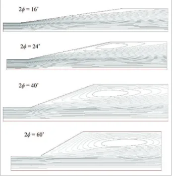
Stream function contours are plotted for all cases, and the results are shown in Figs. 5, 6 and 7. It can be seen that, if the flow has no swirl, there exist flow separation for all tested angles, and the recirculation zone size is proportional to the total angle of the diffuser, being broader when the angle is wider. In the case of swirl addition, some interesting phenomena arise, as follows:
• For S = 0.3, a central recirculating zone appears in the lower angle geometries (i.e. 16° and 24°), indicating the
occurrence of vortex breakdown, although separation of the boundary layer is prevented in these cases. For the 2 wider angles, the separation of boundary layer still occurs. However, swirl delays the growth of boundary layer due to centrifugal forces, and the separation point occurs downstream. his can be conirmed by noting that the recirculating bubble appears further downstream for those cases.
Figure 5. Streamline contours, no swirl.
Figure 7. Streamline contours for S = 0.6.
t h at the recirculation zone increases with increasing
swirl intensity.
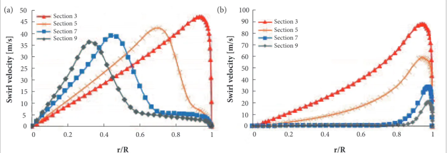
To further analyze this recirculation zone appearing inside the difuser, the swirl velocity proile for various sections throughout the difuser length is plotted against the normalized radius. he sectional planes are indicated in Fig. 8 and, for the various difusers, they are placed at the same xdif/Ldif, so a concise comparison can be made among the diferent geometries. Figure 9 presents the swirl velocity proile along sections 3, 5, 7 and 9, in the case of the difuser with total angle of 60°, for both swirl numbers 0.3 and 0.6. For S = 0.3, it can be noted that the swirl velocity proile develops into a Rankine-vortex type inside the difuser (Najai et al. 2011), although the boundary conditions at the inlet are that of a forced-vortex type, as can be seen for the velocity proile at section 3. he swirl is too weak for the rapid area growth in this case, so the tangential velocity component does not reach the region near the wall because of weak centrifugal forces, achieving a Rankine-vortex type proile. hus, the swirl is not efective in preventing boundary-layer growth and separation in this case, and the axial momentum near the wall is low. On the other hand, for S = 0.6, swirl efect seems to induce centrifugal forces high enough to carry the tangential component to the near-wall region and thus prevent the boundary-layer separation by enhancing momentum transport. In this case, the axial momentum is higher near the wall than when it is close to the centerline, as would be expected by a mass conversation analysis. his makes a recirculation region to appear in the intermediary region instead of near the wall. In addition, the recirculation zone occurring in the intermediary zone, due to the decrease in axial momentum, • For S = 0.6, there exist a central recirculation zone for
all tested geometries, as shown in Fig. 7. Comparing the cases for the 16- and 24°- diffusers, it can be seen
Figure 8. Cross-sections used for velocity proile plots and integrated-weighted-area quantities.
Figure 9. Swirl velocity proiles for 60°- diffuser. (a) S = 0.3; (b) S = 0.6. Section 3
Section 5
Section 9 Section 7
Section 3 Section 5
Section 9 Section 7
r/R r/R
S
w
ir
l
ve
lo
ci
ty
[
m
/s
]
20 40 60 80 90 100
0
0 1
50 70
30
10
0.4
0.2 0.6 0.8
S
w
ir
l
ve
lo
ci
ty
[
m
/s
]
10 30 30 40 45 50
0
0 1
25 35
15
5
0.4
0.2 0.6 0.8
1 2 3 4 5
6 7
8 9 10 11 12
forces the tangential momentum to concentrate in the region
near the wall, as shown in Fig. 9b.
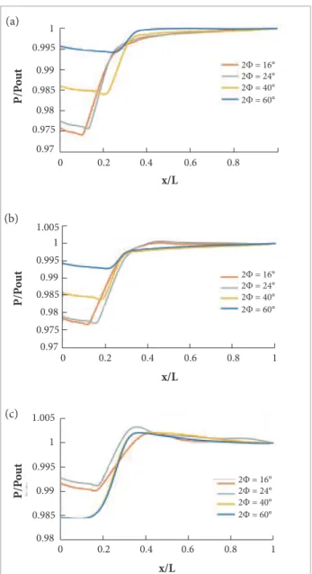
STATIC PRESSURE EVOLUTION
Because swirl addition induces radial pressure gradients, the static pressure is taken as an area-weighted average across the sections presented in Fig. 8 instead of the value in the centerline/ wall, as it is usual for the swirl-free case (where the pressure is assumed constant along cross-section). he static pressure evolution is presented in Fig. 10 and has been normalized by the static pressure at the tailpipe outlet.
x/L
P/P
o
u
t
P/P
o
u
t
P/P
o
u
t
0 0.97 0.975 0.985 0.995
0.98 0.99 1
0.97 0.975 0.985 0.995
0.98 0.99 1 1.005
0.985 0.995
0.98 0.99 1 1.005
0.4
0.2 0.6 0.8
x/L
0 0.2 0.4 0.6 0.8 1
x/L
0 0.2 0.4 0.6 0.8 1
2Φ = 16° 2Φ = 24°
2Φ = 60° 2Φ = 40°
2Φ = 16° 2Φ = 24°
2Φ = 60° 2Φ = 40°
2Φ = 16° 2Φ = 24°
2Φ = 60° 2Φ = 40°
Section 6 Section 5
Section 7
r/R
R
adi
a
l P
ress
ur
e
G
radi
en
t [P
a/m]
0 0
1 10,000
-10,000 20,000 30,000 40,000 50,000 60,000
0.4
0.2 0.6 0.8
Figure 10. Static pressure evolution throughout the diffuser length at different divergence angles. (a) No swirl; (b) S = 0.3; (c) S = 0.6.
In the swirl-free case, Fig. 10a shows that, for all geometries, there is still pressure recovery ater the difuser outlet. his is due to a large-scale mixing in the tailpipe, which converts dynamic pressure into static pressure, as discussed in the literature (Miller 2009). For the case in which S = 0.3, the highest static pressure is achieved at the end of the difuser in the 16- and 24°- geometries, followed by a decrease in the tailpipe. For the 40- and 60°- geometries the pressure still rises ater the difuser due to the large-scale mixing. In the former case, the increase in static pressure due to large-scale mixing is surpassed by the decrease due to losses as a consequence of dissipative mechanisms (wall friction), and therefore the static pressure experiences a net decrease in the tailpipe. For the case in which S = 0.6, all geometries present the same behavior for the static pressure, occurring a maximum recovery at the end of the difuser domain, followed by a decrease through the tailpipe. his is clearly related with the region where the recirculation zone takes place. When it occurs in the intermediary portion of the cross-section, the centrifugal forces pushing the fluid towards the wall are strong, and thus the wall friction losses overcome the pressure recovery due to mixing, causing a net efect of the static pressure decrease. However, when recirculation appears near the wall, the wall friction is low due to the boundary layer separation and therefore the pressure recovery due to large-scale mixing overcomes the pressure loss induced by friction efect.
RADIAL PRESSURE GRADIENT AND WALL SHEAR STRESS
Figure 11 shows the plot of the radial pressure gradient in sections 5, 6 and 7 (Fig. 8) inside the diffuser domain
Figure 11. Radial pressure gradient for 3 geometry
sections at S = 0.3 and 2ϕ = 24°.
Figure 12. Radial pressure gradient for section 5 (geometry
2ϕ = 24°) and 2 different swirl numbers.
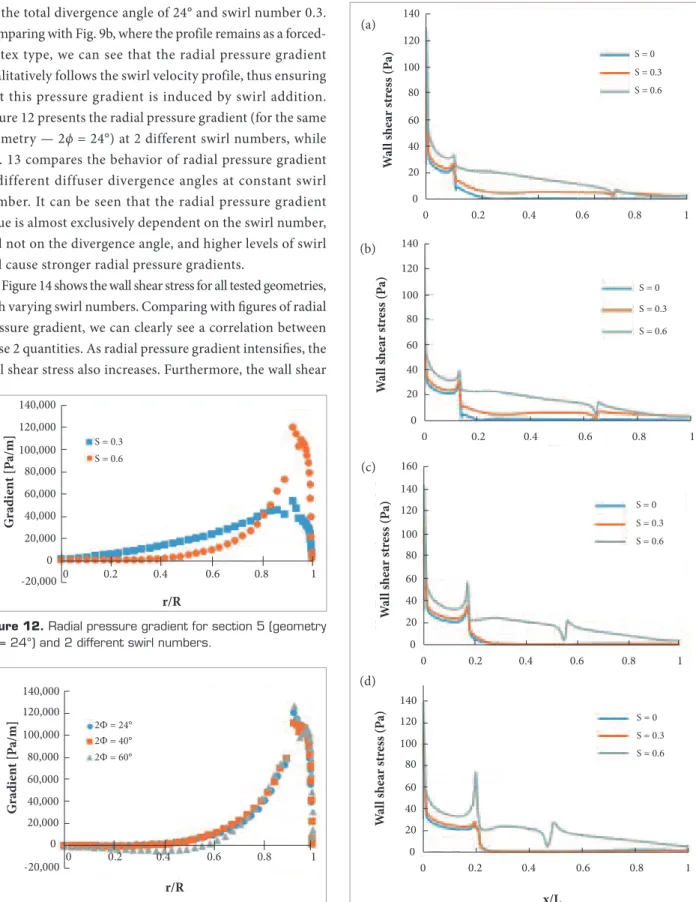
Figure 14. Wall shear stress along the diffuser length.
(a) 2ϕ = 16°; (b) 2ϕ = 24°; (c) 2ϕ = 40°; (d) 2ϕ = 60°.
S = 0
S = 0.3
S = 0.6
x/L W a ll s he a r s tr ess (P a) 20 40 60 80 140 160 100 0 0 1 120 0.4
0.2 0.6 0.8
S = 0
S = 0.3
S = 0.6
x/L W a ll s he a r s tr ess (P a) 20 40 60 80 140 160 100 0 0 1 120 0.4
0.2 0.6 0.8
1
S = 0
S = 0.3
S = 0.6
W a ll s he a r s tr ess (P a) 20 40 60 80 140 100 0 0 1 120 0.4
0.2 0.6 0.8
S = 0
S = 0.3
S = 0.6
x/L W a ll s he a r s tr ess (P a) 20 40 60 80 140 100 0 0 1 120 0.4
0.2 0.6 0.8
Figure 13. Radial pressure gradient for S = 0.6 and 3
different divergence angles.
for the total divergence angle of 24° and swirl number 0.3.
Comparing with Fig. 9b, where the profile remains as a forced-vortex type, we can see that the radial pressure gradient qualitatively follows the swirl velocity profile, thus ensuring that this pressure gradient is induced by swirl addition. Figure 12 presents the radial pressure gradient (for the same geometry — 2ϕ = 24°) at 2 different swirl numbers, while Fig. 13 compares the behavior of radial pressure gradient at different diffuser divergence angles at constant swirl number. It can be seen that the radial pressure gradient value is almost exclusively dependent on the swirl number, and not on the divergence angle, and higher levels of swirl will cause stronger radial pressure gradients.
Figure 14 shows the wall shear stress for all tested geometries, with varying swirl numbers. Comparing with igures of radial pressure gradient, we can clearly see a correlation between these 2 quantities. As radial pressure gradient intensiies, the wall shear stress also increases. Furthermore, the wall shear
r/R R adi a l P ress ur e G radi en t [P a/m] 0 0 1 20,000 -20,000 40,000 60,000 80,000 100,000 120,000 140,000 0.4
0.2 0.6 0.8
2Φ = 24°
2Φ = 60° 2Φ = 40° S = 0.3
S = 0.6
r/R R adi a l P ress ur e G radi en t [P a/m] 0 0 1 20,000 -20,000 40,000 60,000 80,000 100,000 120,000 140,000 0.4
0.2 0.6 0.8
(a)
(b)
(c)
stress is much more inluenced by the swirl number than by
the total divergence angle. his is the same behavior observed in the radial pressure gradient distributions.
The discussion made about the swirl velocity profiles is also implicit from the plots of wall shear stress. For the cases where it develops into a Rankine-vortex profile, the swirl velocity component near the wall is very low, and the wall shear stress almost vanishes in this region. On the other hand, when it remains as a forced-vortex type, the wall shear stresses are high close the wall surface.
CONCLUSIONS
The present study analyzed the influence of swirl addition in the streamline pattern, pressure recovery, pressure gradient, and wall shear stress in a conical diffuser flow. The fact that a central recirculation zone appears in these flows is related to the swirl velocity profile developed inside the diffuser domain. If the swirl intensity is low relatively to the wall divergent angle, the swirl velocity profile develops into a Rankine-vortex profile and thus it is not effective in preventing boundary layer growth and separation. On the other hand, if the swirl intensity is high enough relatively to the wall divergent angle, the swirl velocity profile remains as a forced-vortex type profile and thus prevents boundary layer separation due to: (i) centrifugal forces pushing the fluid toward the wall; and (ii) increase in turbulence intensity in this region, enhancing momentum transport. However, in the last case, the swirl intensity showed also high enough to allow vortex breakdown to occur, generating a central recirculation zone. Although other researchers observed this recirculation zone in their experiments on conical difuser lows, this relationship between swirl velocity proile and wall difuser slope has not been previously mentioned. he results also suggest that there is an optimum swirl intensity where both boundary layer separation and vortex breakdown are prevented, avoiding a decrease in difuser performance due to energy losses. Moreover, this optimum swirl intensity shall be related to the wall slope (i.e. difuser geometry).
An assessment of static pressure evolution throughout the difuser led to the following conclusions. When the swirl velocity proile remains as a forced-vortex type, the wall shear stresses are high due to the centrifugal forces pushing the luid toward the wall, and thus the losses because of friction overcome the pressure recovery due to a large-scale mixing through the tailpipe, resulting in a net decrease in static pressure through the tailpipe. However, when the swirl velocity proile develops into a Rankine-vortex type inside the difuser, the wall shear stresses are low due to separation of boundary layer, and the pressure recovery because of large-scale mixing overcomes the losses due to wall friction, and the pressure still rises throughout the tailpipe. his suggests that, if an optimum swirl intensity is achieved, which prevents both separation and vortex breakdown from occurring, there would be no need of a tailpipe to increase static pressure through a large-scale mixing, as it is usual in practical applications.
Radial pressure gradient and wall shear stresses qualitatively follow the swirl velocity proile. It is indeed expected, as the swirl component is the cause of the appearance of radial pressure gradients and centrifugal forces, which, in turn, moves the luid to the wall, increasing velocity gradients and thus the wall shear stresses. he radial pressure gradient as well as the wall shear stress are much more dependent on the swirl intensity than on the difuser geometry (i.e. total divergence angle).
ACKNOWLEDGEMENTS
The authors would like to acknowledge the Conselho Nacional de Desenvolvimento Cientíico e Tecnológico – Brazil, for their support to this study.
AUTHOR’S CONTRIBUTION
Armfield SW, Cho NH, Fletcher CA (1990) Prediction of turbulence quantities for swirling flow in conical diffusers. AIAA J 28(3):453-460. doi: 10.2514/3.10414
Bigarella E, Azevedo J (2006) Advanced eddy-viscosity and Reynolds-stress turbulence model simulations of aerospace applications. Proceedings of the 24th AIAA Applied Aerodynamics Conference; San Francisco, USA.
Bird RB, Stewart WE, Lightfoot EN (2002) Transport phenomena. 2nd edition. New York: John Wiley & Sons.
Chen KH, Liu NS, Lumley JL (1997) Modeling of turbulent swirling flows. NASA TM-113112.
Cho NH, Fletcher CA (1989) Prediction of turbulent swirling flow in a diffuser with tailpipe. Proceedings of the 10th Australasian Fluid Mechanics Conference; Melbourne, Australia.
Escudier M (1988) Vortex breakdown: observations and expla-nations. Progress in Aerospace Sciences 25(2):189-229. doi: 10.1016/0376-0421(88)90007-3
Escudier M, Keller J (1985) Recirculation in swirling flow: a manifestation of vortex breakdown. AIAA J 23(1):111-116. doi: 10.2514/3.8878
Escue A, Cui J (2010) Comparison of turbulence models in simu-lating swirling pipe flows. Appl Math Model 34(10):2840-2849. doi: 10.1016/j.apm.2009.12.018
ESDU (1990) ESDU 90025: performance of conical diffusers in sub-sonic compressible low; [accessed 2016 Sept 07]. https://www. esdu.com/cgi-bin/ps.pl?sess=unlicensed_1160907142621hkk&-t=doc&p=esdu_90025a
Faler JH, Leibovich S (1977) Disrupted states of vortex flow and vortex breakdown. Phys Fluid 20:1385-1400. doi: 10.1063/1.862033
Galván S, Reggio M, Guibault F (2011) Assessment study of k-ε
turbulence models and near-wall modeling for steady state swir-ling flow analysis in draft tube using Fluent. Engineering Appli-cations of Computational Fluid Mechanics 5(4):459-478. doi: 10.1080/19942060.2011.11015386
Leibovich S (1984) Vortex stability and breakdown: survey and extension. AIAA J 22(9):1192-1206.
McDonald AT, Fox RW, van Dewoestine RV (1971) Effects of swir-ling inlet flow on pressure recovery in conical diffusers. AIAA J 9(10):2014-2018. doi: 10.2514/3.6456
Miller DS (2009) Internal flow systems. 2nd edition. [S.l.]: Miller Innovations.
Najafi A, Mousavian S, Amini K (2011) Numerical investigations on swirl intensity decay rate for turbulent swirling flow in a fixed pipe. Int J Mech Sci 53(10):801-811. doi: 10.1016/j.ijmecs-ci.2011.06.011
Neve RS, Wirasinghe NE (1978) Changes in conical diffuser performance by swirl addition. Aeronaut Q 29(3):131-143. doi: 10.1017/S0001925900008404
Okhio CB, Horton HP, Langer G (1983) Effects of swirl on flow se-paration and performance of wide angle diffusers. Int J Heat Fluid Flow 4(4):199-206. doi: 10.1016/0142-727X(83)90039-5
Okhio CB, Horton HP, Langer G (1986) The calculation of turbulent swirling flow through wide angle conical diffusers and the asso-ciated dissipative losses. Int J Heat Fluid Flow 7(1):37-48. doi: 10.1016/0142-727X(86)90042-1
Pordal HS, Khosla PK, Rubin SG (1993) Pressure flux-split viscous solutions for swirl diffusers. Comput Fluid 22(4-5):663-683. doi: 10.1016/0045-7930(93)90031-4
Rocklage-Marliani G, Schmidts M, Vasantaram V (2003) Three-dimensional laser-Doppler velocimeter measurements in swirling turbulent pipe flow. Flow, Turbulence and Combustion 70(1):43-67. doi: 10.1023/B:APPL.0000004913.82057.81
Sarpkaya T (1974) Effect of the adverse pressure gradient on vor-tex breakdown. AIAA J 12(5):602-607. doi: 10.2514/3.49305
Senoo Y, Kawaguchi N, Nagata T (1978) Swirl flow in conical diffu-sers. B JSME 21(151):112-119.
Sloan DG, Smith PJ, Smoot LD (1986) Modeling of swirl in turbu-lent flow systems. Prog Energ Combust Sci 12(3):163-250. doi: 10.1016/0360-1285(86)90016-X
Yakhot V, Orszag S (1986) Renormalization group analysis of tur-bulence. I. Basic theory. J Sci Comput 1(1):3-51. doi: 10.1007/ BF01061452