ABSTRACT: Two-dimensional lows over harmonically oscillating symmetrical aerofoil at reduced frequency of 0.1 were investigated for a Reynolds number of 135,000, with focus on the unsteady aerodynamic forces, pressure and vortex dynamics at post-stall angles of attack. Numerical simulations using ANSYS® FLUENT CFD solver, validated by wind tunnel experiment, were performed to study the method of sliding mesh employed to control the wing oscillation. The transport of low was solved using incompressible, unsteady Reynolds-Averaged Navier-Stokes equations. The 2-equation k-εrealizable turbulence model was used as turbulence closure. At large angle of attack, complex lows structure developed on the upper surface of the aerofoil induced vortex shedding from the activity of separated lows and interaction of the leading edge vortex with the trailing edge one. This interaction at some stage promotes the generation of lift force and delays the static stall. In this investigation, it was found that the sliding mesh method combined with the k-ε realizable turbulence model provides better aerodynamic loads predictions compared to the methods reported in literature.
KEYWORDS: Aerofoil, Unsteady, Low Reynolds number, Harmonic oscillation, Post-stall, Computational luid dynamics.
Aerodynamics of Harmonically Oscillating
Aerofoil at Low Reynolds Number
Aiman Hakim Abdul Rahman1, Nik Ahmad Ridhwan Nik Mohd1, Tholudin Mat Lazim1, Shuhaimi Mansor1
INTRODUCTION
Among the earliest documented phenomena of dynamic stall, there is the report of Kramer (1932) summarizing his experimental investigation on the efect of vertical gust on a wing stress. he study is also the irst to recognize the dynamic features associated with the rapid variations of incidence experienced by an airfoil (Wernert et al. 1996).
Nowadays, dynamic stall is commonly recognized as the breakdown of the flow field around an oscillating slender lifting surface operating beyond its critical angle of attack (McCroskey 1981). Over a past few decades, the dynamic stall event has become one of the major problems in aeronautics and astronautics. Dynamic stall is a condition where the evolution of the low ield is rather diferent from that obtained for static stall and contains complex unsteady low phenomenon that produces a detrimental efect in many aerodynamic systems. Maneuvering aircrat, helicopter rotor blades, wind turbines, lapping wing of insect, compressor and turbine blades are some examples of engineering application involving unsteady low and unsteady load during operation. Unsteady low is known to produce a negative efect on aerodynamic load, induced vibration, lutter, bufeting (Kim and Chang 2009) and is also known as one of the limiting factors of the aircrat light speed and operation of mechanical system (Lee and Gerontakos 2004). Recently, oscillating wing has gained a particular interest in the ield of biomimetic studies aiming at harvesting propulsive force from circulation low to a small scaled vehicle.
The phenomenon of dynamic stall can be categorized into pre- and post-stall depending on the viscous-inviscid interaction (McCroskey 1981; Kim and Chang 2009; Lee and Gerontakos 2004; McCroskey et al. 1976). Beyond the stall,
1.Universiti Teknologi Malaysia – Faculty of Mechanical Engineering – Aeronautical Laboratory – Skudai/Johor – Malaysia.
Author for correspondence: Nik Ahmad Ridhwan Nik Mohd | Universiti Teknologi Malaysia – Faculty of Mechanical Engineering – Aeronautical Laboratory | 81310 Skudai/Johor – Malaysia | Email: [email protected]
the separation point moves toward the leading edge forming a complicated low structure such as leading edge vortex (LEV), free shear layer, and viscous-inviscid interaction that plays an important role in the characteristics of dynamic stall (Kim and Chang 2009). In helicopter industry, the development of LEV associated with the increase in the pitching moment of rotor blades is undesirable. However, the delay in the LEV detachment from the aerofoil surface provides an increase in dynamic lit to the aircrat (Lee and Su 2011).
Accurate prediction of unsteady low and dynamic stall is still one of challenging tasks in experimental and computational luid dynamics. Numerous experimental papers (McCroskey 1981; Kim and Chang 2009; Lee and Gerontakos 2004; McCroskey et al. 1976; Panda and Zaman 1994; Coton and Galbraith 1999) and numerical investigations (McCroskey and Pucci 1982; Ericsson and Reding 1970; Gaitonde and Fiddes 1993; Dumlupinar and Murthy 2011; Barakos and Drikakis 1999) have been carried out and show that the unsteady low can be separating or reattaching over a large portion of the upper surface of an aerofoil, features which reverse low circulation, formation and shedding of leading and trailing vortex system that induces non-linear luctuating pressure ield and produce transient variation in forces and moments that are diferent to its steady-state conditions (Lee and Gerontakos 2004). he low ield of an aerofoil periodically pitched about a ixed-axis is primarily inluenced by the amplitude αo, the mean angle αm and the frequency of oscillation f . he oscillation frequency is known as the most inluential parameter and is oten presented in terms of reduced frequency — the ratio of 2 time scales: one imposed by the pitching motion and the other by the free stream velocity and the aerofoil chord (Panda and Zaman 1994).
Wang et al. (2010), in their study, employed the dynamic mesh approach for the simulation of harmonically pitching aerofoil following Wernert et al. (1996) for moderate Reynolds number and Lee and Gerontakos (2004) for low Reynolds number cases. he used dynamic mesh technique consists of 2 sub-domains that communicate through a pair of circular common interfaces. he commercial ANSYS® (2013) FLUENT pressure-based solver that solves full unsteady Reynolds-Averaged Navier-Stokes governing equation for incompressible low problem was used. he SIMPLE algorithm was used for the pressure-velocity coupling and the 2nd-order upwind scheme was utilized for the velocity and the turbulence quantities. To accelerate the convergence of the solution, the algebraic multigrid scheme (AMG) with a V-cycle type for the pressure and a lexible type for the momentum was
applied. he turbulence in the low was calculated using the standard k-ω and shear stress transport (SST) k-ωturbulence models with a modiied turbulent viscosity damping.
In Gharali and Johnson (2013), the instantaneous aerodynamic load of a NACA 0012 aerofoil in pure pitching oscillation in a steady freestream was numerically simulated and validated against the experimental research of Lee and Gerontakos (2004), in which the k-ω SST turbulence model with low Reynolds correction similar to that of Wang et al. (2010) was used. he C-grid topology was employed with a total of 20,000 cells and 500 nodes wrapped around the aerofoil. he stability issue that is very sensitive to the value of turbulence intensity (Wang et al. 2010) and mesh skewness (Gharali and Johnson 2013) is also highlighted.
In this paper, the challenges and issues of modelling and understanding the unsteady aerodynamics of an aerofoil at high incidence angles and highly unsteady low using CFD are investigated and presented. he test case is a 2-D aerofoil undergoing fast harmonic oscillations. he solution of the CFD using sliding mesh is then compared against dynamic mesh method and available experimental data.
EXPERIMENTAL METHODS
Wind tunnel or water tunnel becomes one of standard testing procedures in aerodynamic load measurements. To date, various experimental studies on oscillating aerofoil were reported from simple to complicated experimental setup. In this investigation, experimental data obtained from the McGill University’s low speed wind tunnel are referred for validation (Gerontakos 2004; Lee and Gerontakos 2004).
In this experiment, dynamic stall and low characteristics over an oscillating symmetrical NACA 0012 aerofoil at the Reynolds number of 135,000 were investigated. he NACA 0012 aerofoil was made of solid aluminum, with a chord length c of 15 cm and a span of 37.5 m. he origin of the coordinate was located at the leading edge of the aerofoil, which was equipped with 2 endplates with a sharp leading edge to eliminate the 3-D efect at the tip of the wing. he aerofoil pitching axis is located at the ¼ chord. In the test section, the measured turbulent intensity was 0.08% at a free stream velocity u∞= 35 m/s.
downstream of the trailing edge of the aerofoil. For surface pressure measurement, 61 pressure taps (0.35 mmin diameter), in conjunction with 7 fast-response miniature pressure transducers (type YQCH-250-1) staggered 1.5 mmapart in the streamwise direction, were used.
NUMERICAL SIMULATION
In a numerical approach, a similar aerofoil section, as in the wind tunnel experiment of Lee and Gerontakos (2004), was used for validation studies. For unsteady, oscillating aerofoil problem, hybrid unstructured mesh was employed with 2 blocks consisting of stationary and rotating meshes. he Reynolds number used in this investigation was 135,000.
For consistency, the inlet turbulence intensity in CFD was set at 0.08%, similarly to the experiment of Lee and Gerontakos (2004). However, as reported by Wang et al. (2010), the value of the inlet turbulent intensity has some inluence on the stability of the solution. Around the aerofoil, the no-slip boundary condition was employed and wrapped by a boundary layer mesh, which contains 25 layers with the irst cell height set at y+ ≤ 1. To ensure that the viscous efect is properly captured,
an improved method for calculating turbulent boundary layer based on the reference temperature method for turbulence flow was used, resulting in the 1st cell height of less than 5.8 × 10⁻⁵m(Meador and Smart 2005).
In this paper, the ANSYS® (2013) FLUENT CFD that solves unsteady Reynolds-Averaged Navier-Stokes equations for incompressible low problem on unstructured, cell-centered control volume was used. he main purposes of this CFD are the assessment of the sliding mesh method used and blind test for wind tunnel experiment veriication. he used CFD solver takes momentum and pressure as the primary variable and solves pressure correction and momentum sequentially. his type of solver is also known as pressure-based. For time-dependent low problem, the pressure implicit with splitting of operator (PISO) scheme for pressure-velocity coupling was used similarly to the study of Gharali and Johnson (2013). For the selection of turbulence models, similar studies were found in literature using the 2-equation k-ω turbulent model with the transport of shear stress (Gharali and Johnson 2013; Hutchinson et al. 2010; Wang et al. 2010). In Gharali and Johnson (2013), the k-ω turbulence with SST model was used with additional
enhancement in the calculation of the turbulent viscosity damping for low Reynolds number problem.
On the other hand, in this paper, the realizable k-
ε
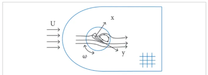
turbulent model (Shih et al. 1995) with enhanced wall treatment and mesh with more than 27,000 points was used and found adequate to resolve the viscous-inviscid interaction as well as able to capture some detail wake structure developed during upstroke and downstroke phases for an aerofoil in post-stall condition. he selection of the realizable k-ε turbulent model was made due to the capability of this turbulent model to accurately predict lows involving rotation, boundary layers under strong adverse pressure gradient, separation and recirculation which oten occur around aerofoil undergoing fast dynamic oscillation and deep stall.he schematic of sliding mesh used in the present study is shown in Fig. 1. he computational domain is divided into 2 blocks. he irst contains stationary mesh and the second, a mesh that rotates at the same frequency as the aerofoil.
he harmonic pitching motion of aerofoil is controlled by sliding mesh method that moves rigidly in a dynamic mesh zone (ANSYS® 2013). For the 2-D problem, the cell zones are connected each other through non-conformal interfaces. he transport equation for a general scalar quantity (ϕ) in moving boundary is solved according to the following equation: Figure 1. Schematics of the numerical setup.
U x
y
ω
where: ρ is the luid density; Γ is the difusion coeicient; u
→ is low velocity vector; →u
g is the mesh velocity of the moving mesh; represents the boundary of control volume ∂V; →A is the face area vector; Sϕ is the source term of ϕ.
each volume forming a discrete equation that expresses the conservation law on a control volume basis. he update in the change in volume is solved using 1st-order backward diference as:
RESULTS AND DISCUSSION
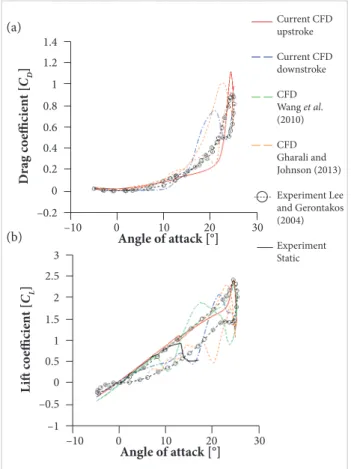
In this section, aerodynamic loads in terms of lit and drag coeicients of a NACA 0012 aerofoil undergoing harmonic oscillation at a reduced frequency, k = 0.1, are presented with the intention to evaluate the combination of sliding mesh approach and the used k-ε realizable turbulence model.
Figures 2a and 2b show the comparison of the instantaneous lit and drag coeicients hysteresis calculated for a 1 harmonic oscillation cycle. From these igures, the harmonic motion of the aerofoil in the upstroke phase extends the aerofoil stall angle beyond the static stall and up to the angle of attack α = 24.4°,as predicted in CFD and the experiment. he predicted maximum lit coeicient is reported to be CL= 2.4 at α = 24.43°and 2.5 times higher than the static stall. he linear lit region also extended up to the angle of attack α = 20°with the gradient of the dCL/dα maintained similar to the static case. In upstroke phase, CFD predicts that there is slightly loss in lit within 20° ≤ α(t) ≤ 25°(↑). In the dynamic stall region, the wing where: n and n + 1 denote the respective quantity at
the current and next time level; dV/dt is the volume-time derivative of the control volume.
For sliding mesh approach, the mesh in sliding region remains in its original shape and volume and does not change in time. hus Eq. 2 can be written as:
Using Eq. 3, the 1st term in Eq. 1 can be written as:
In order to satisfy the mesh conservation law, the volume-time derivative of the control volume is computed from the dot product of mesh velocity and face area vector →u g ∙ A A →:
he results presented in this paper refer to the aerofoil subjected to a harmonic oscillation which is deined as a function of the angle of attack variation, α(t) = αm+ αo sin(ωt), where ω is the oscillation frequency.In the case of oscillating aerofoils, the unsteady motion is characterized by the non-dimensional similarity parameter known as reduced frequency of oscillation, deined by k = ωc/2U∞, where U∞ is the freestream velocity. he aerofoil axis of oscillation is located at ¼ chord point.
The test cases presented are related to aerofoil at post-stall condition with instantaneous angle of attack, α(t) = 10° + 15° sin(ωt), and reduced frequency, k = 0.1, was chosen. he simulations were run for one and a half cycle with time step dt = 0.0006 s. In later discussion, lift and drag forces on aerofoil are described in terms of the non-dimensionalized unit deined as CL= Fy /(0.5ρU∞2c) and C
D= Fx /(0.5ρU∞
2c),
respectively, where Fy and Fx are the lit and drag forces.
Figure 2. Instantaneous aerodynamic loads hysteresis for
test case: α(t) = 10° + 15° sin(ωt), k = 0.1. (a) Drag coeficient;
(b) Lift coeficient. –10 –0.2
0 0.2 0.4 0.6 0.8 1 1.2 1.4
Current CFD upstroke
Current CFD downstroke
CFD Wang et al. (2010)
CFD Gharali and Johnson (2013)
Experiment Lee and Gerontakos (2004)
Experiment Static
10 20 30
0
Angle of attack [°]
Dr
ag c
o
effi
ci
en
t [
CD
]
–10 –1 –0.5 0 0.5 1 1.5 2 2.5 3
10 20 30
0
Angle of attack [°]
L
ift c
o
effi
ci
en
t [
CL
]
(2)
(3)
(4)
(5) (a)
stall has a similar pattern and magnitude of loss in lit force to that reported in the experiment and in Wang et al. (2010). However, the dynamic stall event and the loss in the lift force as predicted in Wang et al. (2010) showed that there is continuing loss in lit beyond the dynamic stall angles as reported in the experiment. Gharali and Johnson (2013), on the other hand, show that the used CFD methods inaccurately predict the dynamic stall angle, which was found to occur earlier than reported in the experiment. Similarly to Wang et al. (2010), the present CFD analysis predicts a gain in lit as the aerofoil enters in the downstroke phase. Moreover, in Wang et al. (2010), the gain in lit appeared to occur at slightly lower incidence angles unlike the present study. As can be seen in Fig. 2b, the present analysis shows that the used CFD method slightly underpredicts the drag coeicient within 15° ≤ α(t) ≤ 22°(↑). A steep increase in the predicted drag can also be seen in the downstroke phase as a result of large increase in the predicted lit (Fig. 2b) but occurs at lower incidence aerofoil angles as compared to the investigation of Gharali and Johnson (2013).
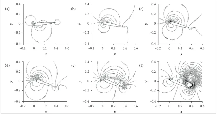
Variation in the predicted lit and drag was found to be strongly associated with the change in the local surface pressure with respect to time. Figures 3 and 4 show the instantaneous ield pressure near the aerofoil in upstroke and downstroke phases,
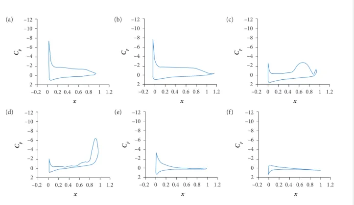
respectively. For the purpose of comparison, the ield pressures shown in these igures are extracted for the same pressure range. In upstroke phase and at a low angle of attack up to 6°, the ield pressure (Fig. 3) and the surface pressure (Fig. 5) suggest that the low is mostly attached to the surface. As the aerofoil continues moving upward, with the incidence angle reaching approximately 21°(linear region of lit in dynamic condition), the sudden decrease in the suction pressure is apparent on the upper surface, near the leading edge (Fig. 3d). his sudden decrease in the ield pressure near the suction area can also be visualized by a large negative pressure gradient near the leading edge of the aerofoil. his phenomenon can also be associated with the generation and propagation of LEV that dominates the upper surface of an aerofoil. As the incidence angle continues to increase, the LEV starts to detach from the surface as well as to propagate and travel downstream towards the trailing edge (Fig. 3e). his LEV carries low pressure ield and its close proximity to the surface of an aerofoil greatly alters the value of the aerofoil local surface pressure. As the LEV and trailing edge vortex (TEV) interact with each other, it causes a large drop in ield pressure near the trailing edge region (Figs. 3f and 5f).
In the transition phase (from upstroke to downstroke), the used method predicts a steep lost in the lit known as dynamic stall. In this transition phase, the primary LEV and
Figure 3. Instantaneous ield pressure coeficient in upstroke phase. (a) −4.85°, t = 3,000 s, ↑;(b) 12.42°, t = 100 s, ↑;
(c) 16.99°, t = 300 s, ↑;(d) 20.85°, t = 500 s, ↑;(e) 23.58°, t = 700 s, ↑;(f) 24.98°, t = 1,000 s, ↑.
0.4
0.2
0
–0.2
–0.4
–0.2 0 0.2 0.6
x
y
0.4
0.4
0.2
0
–0.2
–0.4
–0.2 0 0.2 0.6
x
y
0.4
0.4
0.2
0
–0.2
–0.4
–0.2 0 0.2 0.6
x
y
0.4
0.4
0.2
0
–0.2
–0.4
–0.2 0 0.2 0.6
x
y
0.4
0.4
0.2
0
–0.2
–0.4
–0.2 0 0.2 0.6
x
y
0.4
0.4
0.2
0
–0.2
–0.4
–0.2 0 0.2 0.6
x
y
0.4
(a)
(d)
(b)
(e)
(c)
Figure 4. Instantaneous ield pressure coeficient in downstroke phase. (a) 23.98°, t = 1,200 s, ↓;(b) 22.93°, t = 1,300 s, ↓;
(c) 19.84°, t = 1,500 s, ↓;(d) 17.88°, t = 1,600 s, ↓;(e) 11.03°, t = 1,900 s, ↓;(f) −4.99°, t = 2,900 s, ↓.
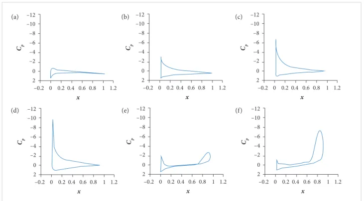
Figure 5. Instantaneous surface pressure coeficient (C
P) distribution in upstroke phase. (a) −4.85°, t = 3,000 s, ↑;(b) 12.42°,
t = 100 s, ↑;(c) 16.99°, t = 300 s, ↑;(d) 20.85°, t = 500 s, ↑;(e) 23.58°, t = 700 s, ↑;(f) 24.98°, t = 1,000 s, ↑.
0.4
0.2
0
–0.2
–0.4
–0.2 0 0.2 0.6
x
y
0.4
0.4
0.2
0
–0.2
–0.4
–0.2 0 0.2 0.6
x
y
0.4
0.4
0.2
0
–0.2
–0.4
–0.2 0 0.2 0.6
x
y
0.4
0.4
0.2
0
–0.2
–0.4
–0.2 0 0.2 0.6
x
y
0.4
0.4
0.2
0
–0.2
–0.4
–0.2 0 0.2 0.6
x
y
0.4
0.4
0.2
0
–0.2
–0.4
–0.2 0 0.2 0.6
x
y
0.4
–12 –10 –8 –6 –4 –2 0 2
–0.2 0 0.2 1 1.2
x
Cp
0.4 0.6 0.8
–12 –10 –8 –6 –4 –2 0 2
–0.2 0 0.2 1 1.2
x
Cp
0.4 0.6 0.8
–12 –10 –8 –6 –4 –2 0 2
–0.2 0 0.2 1 1.2
x
Cp
0.4 0.6 0.8
–12 –10 –8 –6 –4 –2
0 2
–0.2 0 0.2 1 1.2
x
Cp
0.4 0.6 0.8
–12 –10 –8 –6 –4 –2 0 2
–0.2 0 0.2 1 1.2
x
Cp
0.4 0.6 0.8
–12 –10 –8 –6 –4 –2 0 2
–0.2 0 0.2 1 1.2
x
Cp
0.4 0.6 0.8
TEV begin to detach from the aerofoil surface, forming vortex shedding in the wake downstream of the aerofoil (Fig. 4a).
(a) (a)
(d) (d)
(b) (b)
(e) (e)
(c) (c)
(f) (f)
–12 –10 –8 –6 –4 –2
0 2
–0.2 0 0.2 1 1.2
x
Cp
0.4 0.6 0.8
–12 –10 –8 –6 –4 –2 0 2
–0.2 0 0.2 1 1.2
x
Cp
0.4 0.6 0.8
–12 –10 –8 –6 –4 –2 0 2
–0.2 0 0.2 1 1.2
x
Cp
0.4 0.6 0.8
–12 –10 –8 –6 –4 –2 0 2
–0.2 0 0.2 1 1.2
x
Cp
0.4 0.6 0.8
–12 –10 –8 –6 –4 –2 0 2
–0.2 0 0.2 1 1.2
x
Cp
0.4 0.6 0.8
–12 –10 –8 –6 –4 –2 0 2
–0.2 0 0.2 1 1.2
x
Cp
0.4 0.6 0.8
condition were numerically simulated using the sliding mesh method and k-ε realizable turbulent model. The purposes of this research were to investigate the potential of sliding mesh and k-ε realizable turbulent model in the simulation of aerofoil in unsteady oscillation, in order to support wind tunnel experiment, to fully understand the aerodynamic behavior of aerofoils in harmonic oscillation and for the design of control system for lexible wing. Overall, the cyclical forces and low structure, including LEV and TEV interaction, propagation and shedding, agreed very well qualitatively and quantitatively with those reported in literature.
It can also be concluded that, for low Reynolds number problems, the sliding mesh strategy accompanied by the used 2-equation k-ε realizable turbulence model provides better aerodynamic loads prediction compared to the moving mesh approach using the k-ωSST. he k-ε realizable turbulence model is also found to be adequate in capturing the low ield at high incidence angles and during dynamic stall conditions comparable to the experiment. In the upstroke cycle and at high aerofoil incidence angles, the propagation and the close proximity of the LEV to the aerofoil surface cause a large drop in the static
Figure 6. Instantaneous surface pressure coeficient (C
P) distribution in downstroke phase. (a) 23.98°, t = 1,200 s, ↓;
(b) 22.93°, t = 1,300 s, ↓;(c) 19.84°, t = 1,500 s, ↓;(d) 17.88°, t = 1,600 s, ↓;(e) 11.03°, t = 1,900 s, ↓;
(f) −4.99°, t = 2,900 s, ↓.
(a)
(d)
(b)
(e)
(c)
(f) LEV propagates and travels downward, a secondary LEV is
developed due to the downward movement of the aerofoil. he progression of LEV from leading to trailing edge of the aerofoil again develops a low pressure area on the upper surface resulting in an increase in the normal and axial forces. his is clearly visible at an aerofoil incidence angle of approximately 20° (↓). his is beneited from a large pressure loss because LEV (clockwise rotation) and TEV (anti-clockwise rotation) activities occur on the upper surface of theaerofoil. he surface static pressure coeicients for an aerofoil in downstroke phase are depicted in Figs. 6a to 6f. hese igures also show that, even for a geometrically symmetrical aerofoil, the aerodynamics and low characteristics in the upstroke phase are heterogeneous to the downstroke phase.
CONCLUSION
pressure on the upper surface of the aerofoil, and this is predicted to occur approximately at ½ of aerofoil chord. he large deicit in static pressure may cause some inluence in the aerofoil pitching moment. For future studies, the detail of LEV-TEV interaction, boundary layer profile, separation and attachment will be investigated to fully understand the low characteristics in the viscous-sublayer region leading to turbulent low.
ACKNOWLEDGEMENTS
The authors would like to thank the Universiti Teknologi Malaysia, for the financial support to the current study
through Flagship Research Grant No: Q.J130000.2424.01G92, as well as Mr. Hasrizam, for preparing mesh and computer setup.
AUTHOR’S CONTRIBUTION
Mohd NARN administered, designed, and made the setup of the numerical simulation as well as wrote the manuscript. Lazim TM and Mansor S provided technical support and conceptual advices. Rahman AHA performed the numerical setup, the data analysis and wrote the manuscript. All authors contributed equally to this paper.
REFERENCES
ANSYS® (2013) ANSYS FLUENT theory guide. Canonsburg: ANSYS, Inc.
Barakos G, Drikakis D (1999) An implicit unfactored method for unsteady turbulent compressible lows with moving boundaries. Comput Fluids 28(8):899-922. doi: 10.1016/S0045-7930(98)00057-7
Coton FN, Galbraith RA (1999) An experimental study of dynamic stall on a inite wing. Aeronaut J 103(1023):229-236. doi: 10.1017/ S0001924000027895
Dumlupinar E, Murthy VR (2011) Investigation of dynamic stall of airfoils and wing. Proceedings of the 29th AIAA Applied Aerodynamics Conference; Honolulu, USA.
Ericsson LE, Reding JP (1970) Unsteady airfoil stall review and extension. Proceedings of the 8th AIAA Aerospace Sciences Meeting; New York, USA.
Gaitonde A, Fiddes S (1993) A moving mesh system for the calculation of unsteady lows. Proceedings of the 31st Aerospace Sciences Meeting; Reno, USA.
Gerontakos P (2004) An experimental investigation of low over an oscillating airfoil (Master’s thesis). Montreal: McGill University.
Gharali K, Johnson DA (2013) Dynamic stall simulation of a pitching airfoil under unsteady freestream velocity. J Fluid Struct 42:228-244. doi: 10.1016/j.jluidstructs.2013.05.005
Hutchinson SR, Brandner PA, Binns JR, Henderson AD, Walker GJ (2010) Development of a CFD model for an oscillating hydrofoil. Proceedings of the 17th Australasian Fluid Mechanics Conference; Auckland, New Zealand.
Kim DH, Chang JW (2009) Reynolds number effects on unsteady boundary layer of an oscillating airfoil. Proceedings of the 27th AIAA Applied Aerodynamics Conference; San Antonio, USA.
Kramer M (1932) Increase in the maximum lift of an airplane wing due to sudden increase in its effective angle of attack resulting from
a gust. Washington: National Advisory Committee for Aeronautics .Memorandum No.: TM 678.
Lee T, Gerontakos P (2004) Investigation of low over an oscillating airfoil. J Fluid Mech 512:313-341. doi: 10.1017/S0022112004009851
Lee T, Su YY (2011) Unsteady airfoil with a harmonically delected trailing-edge lap. Journal of Fluids and Structures 27(8):1411-1424. doi: 10.1016/j.jluidstructs.2011.06.008
McCroskey WJ (1981) The phenomenon of dynamic stall. Moffett Field: NASA Ames Research Center. Memorandum No.: TM 81-264.
McCroskey WJ, Carr LW, McAllister KW (1976) Dynamic stall experiments on oscillating airfoils. AIAA J 14(1):57-63. doi: 10.2514/3.61332
McCroskey WJ, Pucci SL (1982) Viscous-inviscid interaction on oscillating airfoils in subsonic low. AIAA J 20(2):167-174.
Meador WE, Smart MK (2005) Reference enthalpy method developed from solutions of the boundary-layer equations. AIAA J 43(1):135-139.
Panda J, Zaman KBMQ (1994) Experimental investigation of the low ield of an oscillating airfoil and estimation of lift from wake surveys. J Fluid Mech 265:65-95. doi: 10.1017/S0022112094000765
Shih TH, Liou W, Shabbir A, Yang Z, Zhu J (1995) A new k - ε eddy viscosity model for high Reynold number turbulent lows: model development and validation. Comput Fluid 24(3):227-238.
Wang S, Toa Z, Ma L, Ingham D, Pourkashanian M (2010) Numerical investigation on dynamic stall associated with low Reynolds number lows over airfoils. Proceedings of the IEEE 2nd International Conference on Computer Engineering and Technology; Reno, USA.