Lat. Am. j. solids struct. vol.13 número7

(1)

Abstract

Thermal effects can be one of the most harmful conditions that any steel structure should expect throughout its service life. To counteract this effect, a new beam, with a capability to dissipate thermally induced axial force by slanting of end-plate connection at both ends, is proposed. The beam was examined in terms of its elastic mechanical behavior under symmetric transverse load in presence of an elevated temperature by means of direct stiffness finite element model. The performance of such connection is de-fined under two resisting mechanisms; by friction force dissipation between faces of slant connection and by small upward crawling on slant plane. The presented numerical method is relatively easy and useful to evaluate the behavior of the proposed beam of vari-ous dimensions at different temperatures. Its applicability is evi-dent through satisfactory results verification with those from ex-perimental, analytical and commercially available finite element software. Based on the good agreement between theoretical and experimental methods, a series of design curves were developed as a safe-practical range for the slant end-plate connections which are depend on the conditions of the connection.

Keywords

Slanted end-plate connection, elevated temperature, symmetric transverse load, direct stiffness finite element model, analytical model.

Numerical Study on the Structural Performance of Steel

Beams with Slant End-plate Connections

1 INTRODUCTION

The search for an economical resistance method to improve the performance of steel structures due to elevated temperature remains a challenging task that captures the interest of structural engineers in recent decades. Commonly employed existing engineering solutions to address temperature relat-ed concerns are in the forms of increasing section area, provision of lateral supports (Usmani et al.,

Farshad Zahmatkesh a Mohd. H. Osman a Elnaz Talebi b Ahmad B.H. Kueh b Mahmood. Md. Tahir b *

a_{UTM Forensic Engineering Centre,} Universiti Teknologi Malaysia (UTM), 81310 UTM Johor, Malaysia.

b_{UTM Construction Research Centre,} Universiti Teknologi Malaysia (UTM-CRC), 81310 UTM Johor, Malaysia,

*_{Mahmoodtahir@utm.my}

http://dx.doi.org/10.1590/1679-78252158

(2)

(3)

expan-sion at initial stages of the thermal loading. In much the same vein, numerical study of beam– column joints under thermal load using numerous types of connections had been carried out by Yang and Tan (2012), from which the static solver remains a more accurate tool compared to that of explicit in obtaining structural response although non-convergence can be an issue when dealing with fracture simulation in the former. They commented that changes in the arrangement of bolts in flush end plate connections can improve the structural performance, and that current acceptance criteria of rotation capacities for steel joints are somewhat too conservative as they only consider pure flexural resistance. Accordingly, new connection acceptance criteria were proposed. In addition to available numerical works, Qian et al. (2008) conducted an experimental investigation of steel extended end-plate beam-to-column joints at elevated temperatures at 400, 550, and 700°C with different axial compression forces applied to the beams to simulate restraint effects. It was observed that axial restraint force plays a principal role on the steel joint moment capacity, and that there was a clear beam web tension field action near the column in thermally unrestrained cruciform tests. The fundamental development of an analytical model of such a connection when subjected to a non-symmetric gravity load and a temperature increase has been formulated by Zahmatkesh et al. (2014b). It was demonstrated from the study that an increase in temperature in the beam with a general vertical bolted connection induces a huge extra axial force that decreases the capability in carrying external gravity loads. Also, this study showed that by changing the connection to that of slanting type, this additional axial force can be damped efficiently.

These literatures have clearly identified that the chief concern in steel structures under thermal load lies in the connection details and restraining method. It is worthwhile to note that most exist-ing studies on steel beams have only considered the structural response in the use of conventional vertical end-plate connection due to applied thermal axial forces. So far, there is little evidence that suggests a structural method to reduce the amount of axial force in restrained beams when subject-ed to elevatsubject-ed temperature. Also, there has been no controllsubject-ed study comparing differences in the thermal responses of vertical (conventional) and slanted end-plate connections for steel beams.

(4)

2 VERTICAL AND SLANT END-PLATE CONNECTION CHARACTERISTICS OF BEAM

SUBJECTED TO TEMPERATURE INCREASE

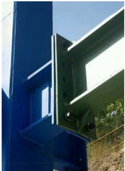
Figures 1 and 2 show the structural arrangements of vertical and test scale of slant end-plate con-nection systems respectively. The popularity of bolted end-plate concon-nections is largely due to its simplicity in fabrication and installation. In general, these connections consist of end-plates that are welded to the ends of a beam in the workshop and then bolted to the flange of columns on site. They are usually used in industrial structures, residential towers in terms of knee connections with end-plate and beam connections in gable roofs. The maximum angle of slanting end-plate connec-tion (Figure 2) has been set to 60°, because a higher angle is not practical for crossing bolts into the holes at the top and bottom of end-plate for fastening (Zahmatkesh et al., 2014c).

Figure 1:Steel beam system with vertical bolted end-plate connections.

Slant end-plate

(5)

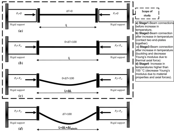
The beam with restrained supports tends to have expansion when it is subjected to temperature increase. So, if the supports do not allow enough tolerance for motion, their reactions will apply huge axial forces in the beam. Most of the times, elongation of members in the elastic regime of material is small. Therefore, the introduction of the slant end-plate connection can damp the exist-ing axial force by allowexist-ing the ends of beam to crawl on the connection surface due to elongation of the beam. Hypotheses about the stages of the performance and the reaction of end-plate connections due to increase in temperature are shown in Figures 3 and 4, for vertical and slant types, respective-ly. As shown in Figure 3, after an increase in temperature, the beam generally tends to buckle due

to increase in axial load (Pcr), because vertical end-plate connection does not allow the beam to

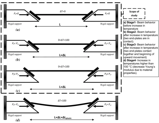
have expansion. On the other hand, as shown in Figure 4, the supports reactions apply axial forces after temperature increase to the beam through member expansion such that the slant surface al-lows the beam to damp axial force and expansion by means of linear crawling on the slant surface. Although there is a vertical motion tolerance between the surfaces in vertical end-plate connections, it is unable to absorb the expansion of two ends of the beam in the horizontal direction because the direction of expansion is perpendicular to the direction of moving surface. In the slant end-plate connection, there is a slanting tolerance between the surfaces such that it can absorb the expansion of two ends of the beam using crawling mechanism over the slanting faces, because the direction of horizontal expansion can be propelled to the slanting plane of connection.

L

Rigid support Rigid support

∆T=

Pt=0 Pt=0

L

Pt< Pcr Pt< Pcr

<∆T<

L+∆L

∆T> (a)

(b)

Pt> Pcr Pt> Pcr

(c)

<∆T<

L+∆L+∆Lplastic

Pt> Pcr Pt> Pcr

(d)

Scope of study

a) Stage1-Beam connections before increase in

temperature,

b) Stage2-Beam connection after increase in temperature (contact two end-plates together)

c) Stage3-Beam connection after increase in temperature (buckling and decrease Young’s modulus due to thermal axial force)

d) Stage4- Increase in temperatures higher than 100 °C (decrease Young’s modulus due to material properties and axial forces).

(6)

L

∆T=

Pt=0 Pt=0

L+∆L

Pt< Pcr Pt< Pcr

L+∆L

<∆T<

Pt≤ Pcr Pt≤ Pcr

<∆T<

L+∆L+∆Lplastic

∆T>

Pt> Pcr Pt> Pcr

(a)

(b)

(c)

(d)

Scope of study

a) Stage1- Beam behavior before increase in temperature

b) Stage2- Beam behavior after increase in temperature (two end-plates are in contact).

c) Stage3- Beam behavior after increase in temperature (two end-plates contact together and beginning of upward movement)

d) Stage4- Increase in temperatures higher than 100 °C (decrease Young’s modulus due to material properties).

Figure 4:Beam with slant end-plate connection subjected to temperature increase.

3 DIRECT STIFFNESS FINITE ELEMENT FORMULATION

3.1 Case Study Description

In the current formulation, three case studies are simulated in two common categories; before ther-mal effect and after uniform elevated temperature. In the first case study, it is assumed that the two ends of the beam are supported with rollers on a fixed slanting plane that can carry the mo-ment. The second case study is similar to the first case but its difference is there exists now a fric-tion force between the two end-plates. In the third case study, we consider the use of the fricfric-tion bolts in the beam with slant end-plate connection. The effects of various types of friction factors and slanting angles are to be investigated. The results from the direct stiffness formulation are first validated by an experimental test for selected cases. To expand study to all cases, results from the direct stiffness method and the modeling using the commercial finite element package, ABAQUS 6.9, are compared with those of analytical equations given by Zahmatkesh et al. (2014b).

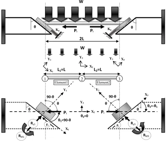
3.2 The Connection with Roller Supports

(7)

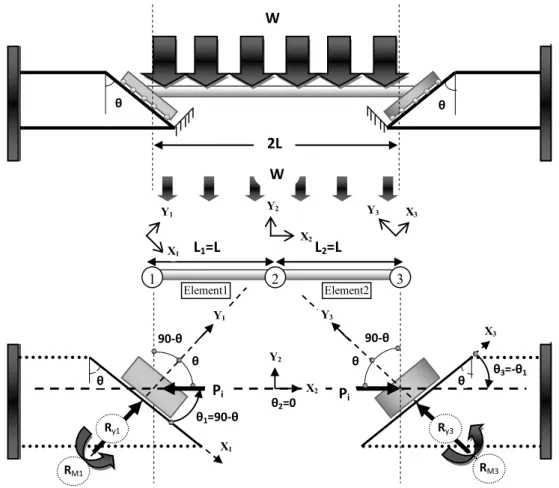
move-ment while the other ends are free as shown in Figure 5. The supports are rollers on slanted lines, so that the beam is in static equilibrium before thermal effect. In the static equilibrium, the uniform symmetric transverse load, W, causes the roller end-plates to move downward, but the initial axial load in the beam, Pi, resists against downward sliding. Therefore, in this case study, if any com-pression axial force due to elevated temperature is applied, the end-plates tend to move upward without any resistive force from support reaction such as friction. The boundary condition (B.C.) of roller supports can channel the total elongation of beam by free sliding upward over the slanting surface. As a result, the amount of axial force due to elevated temperature goes to zero and is damped completely. For model description, the beam member in Figure 5 is divided into two ele-ments and three joints (nodes) such that the length of each element is equal to L with the same properties of section (cross-sectional area, A, and second moment of area, I) and material (Young’s modulus, E). For convenience of displacements and reaction forces computations, local axes defini-tions that follow the slant plane are adopted: X1-Y1 at the left and X3-Y3 at the right hand sides and X2-Y2 local axes at node 2 that is coincided with the global axes. From the standard stiffness

matrix of general frame element, Kelement, and the transformation matrices, T1 and T2, the stiffness

matrices of elements, K1 and K2, at local axes can be obtained from Equations 1 and 2. Note that local axes are used instead of global axes to obtain force and displacement at the slanting direction.

The angle of beam element with the left support in the X1-Y1 local axes is equal to �1, and it is

equal to �3 at the right support in the X3-Y3 local axes. In the model, the angle of end-plate with

the vertical on the left hand side is considered similar to that of the right hand side (�).

1 1 1

T

K  T

K

T

       

       

(1)

2 2 2

T

K  T

K

T

       

       

(2)

Where

1 1

2 2

cos sin 0 0 0 0 sin cos 0 0 0 0

0 0 1 0 0 0

0 0 0 cos sin 0 0 0 0 sin cos 0

0 0 0 0 0 1

1 T

 



 





























(3)

2 2

3 3

cos sin 0 0 0 0 sin cos 0 0 0 0

0 0 1 0 0 0

0 0 0 cos sin 0 0 0 0 sin cos 0

0 0 0 0 0 1

2 T

 



 





























(8)

l

θ θ

W

θ θ

θ

Ry

θ

L =L L =L

1 2 3

Element1 Element2

Y2

X2 X1

Y1 Y3 X3

X1 Y1

X3 Y3

Y2

X2

θ =9 ‐θ θ =

θ =‐θ

Ry3

9 ‐θ 9 ‐θ

RM RM3

W L

Pi

Figure 5:Force diagram of beam with slant end-plate connections due to symmetric transverse load and increase in temperature (frictionless support).

Standard stiffness matrix of general frame element:

3 2 3 2

2 2

3 2 3 2

2 2

0 0 0 0

12 6 12 6

0 0

6 4 6 2

0 0

0 0 0 0

12 6 12 6

0 0

6 2 6 4

0 0

lement

EA EA

L L

EI EI EI EI

L L L L

EI EI EI EI

L L L L

e

EA EA

L L

EI EI EI EI

L L L L

EI EI EI EI

L L L L

K K



  



 





















































(5)

(9)

2

3 3 2 3 3

3 3 2 3

2 2

1 1 1 1 1 1 1 1 2 1 2 1 2 2 1 1

2 2

1 1 1 1 1 1 1 2 1 1 2 1 2 1 2

12 12 6 12 12 6

12 12 6 12

( ) ( ) ( ) ( ) ( ) ( ) ( ) ( ) ( ) ( )

( ) ( ) ( ) ( ) ( ) ( ) ( ) ( )

1

EA EI EA EI EI EA EI EA EI EI

L L L L L L L L L L

EA EI EA EI EI EA EI EA

L L L L L L L L

c s c s c s s c c s s c s c s s

c s c s s c c c s c s s s c c

K                2 3

2 2 2 2

3 3 2 3 3 2

3

1

1 1 2 2

2 2

1 2 1 2 2 1 1 2 2 2 2 2 2 2 2 2

1 2 2 1 1 2

12 6

6 6 4 6 6 2

12 12 6 12 12 6

12 ( ) ( ) ( ) ( ) ( ) ( ) ( ) ( ) ( ) ( ) ( ) ( ) ( ) ( ) ( ) ( ) ( ) ( ) ( EI EI L L

EI EI EI EI EI EI

L L L L L L

L L L L L L L L L L

EA EI EA

L L

c

s c s c

c c s s c s c s s c s c s c s s

c s c s s s

 

     

  

2

3 2 3 3 2

2 2 2

2 2

1 2 2 2 2 2 2 2 2 2

1 1 2 2

12 6 12 12 6

6 6 2 6 6 4

) ( ) ( ) ( ) ( ) ( ) ( ) ( )

( ) ( ) ( ) ( )

EI EI EA EI EA EI EI

L L L L L L L L

EI EI EI EI EI EI

L L L L L L

c c c c s c s s c c

s c s c

                                                   (6) 2

3 3 2 3 3

3 3 2 3

2

2 2

2 2 2 2 2 2 2 2 3 2 3 2 3 3 2 2

2 2

2 2 2 2 2 2 2 3 2 2 3 2 3 2 3

12 12 6 12 12 6

12 12 6 12

( ) ( ) ( ) ( ) ( ) ( ) ( ) ( ) ( ) ( )

( ) ( ) ( ) ( ) ( ) ( ) ( ) ( )

L L L L L L L L L L

EA EI EA EI EI EA EI EA

L L L L L L L L

c s c s c s s c c s s c s c s s

c s c s s c c c s c s s s c c

K                2 3

2 2 2 2

3 3 2 3 3 2

3

2

2 2 3 3

2 2

2 3 2 3 3 2 2 3 3 3 3 3 3 3 3 3

2 3 3 2 2 3

12 6

6 6 4 6 6 2

12 12 6 12 12 6

12 ( ) ( ) ( ) ( ) ( ) ( ) ( ) ( ) ( ) ( ) ( ) ( ) ( ) ( ) ( ) ( ) ( ) ( ) ( EI EI L L

EI EI EI EI EI EI

L L L L L L

L L L L L L L L L L

EA EI EA

L L

c

s c s c

c c s s c s c s s c s c s c s s

c s c s s s

 

     

  

2

3 2 3 3 2

2 2 2

2 2

2 3 3 3 3 3 3 3 3 3

2 2 3 3

12 6 12 12 6

6 6 2 6 6 4

) ( ) ( ) ( ) ( ) ( ) ( ) ( )

( ) ( ) ( ) ( )

EI EI EA EI EA EI EI

L L L L L L L L

EI EI EI EI EI EI

L L L L L L

c c c c s c s s c c

s c s c

                                                   (7) Where

1

cos ,

₁

c





Hence, the total equilibrium equation for the beam takes the following form.

1 1 1 1 1 1

11 12 13 14 15 16

1 1 1 1 1 1

21 22 23 24 25 26

1 1 1 1 1 1

31 32 33 34 35 36

1 1 1 1 2 1 2 1 2 2 2 2

41 42 43 44 11 45 12 46 13 14 15 16

1 1 1 1 2 1 2 1 2 2 2 2

51 52 53 54 21 55 22 56 23 24 25 26

1 1 1 1

61 62 63 64

0 0 0

K K K K K K

K K K K K K K K K K K K

K K K K

       1 1 2 2

2 1 2 1 2 2 2 2

2

31 65 32 66 33 34 35 36

2 2 2 2 2 2

3

41 42 43 44 45 46

2 2 2 2 2 2

3

51 52 53 54 55 56

2 2 2 2 2 2

3

61 62 63 64 65 66

1

0 0 0

dx R dy dr dx dy dr

K K K K K K K K

dx

K K K K K K

dy

K K K K K K

dr

K K K K K K

  

















































































_

_





1 1 1 1 1 1 2 2 2 2 2 2 3 3 3 3 3 3 x fx Ry fy Rm fm Rx fx Ry fy Rm fm Rx fx Ry fy Rm fm 



 





 





 





 





 





 





 





 





 





 





 





 





 





 



(9)

(10)

Where

(10)

are the displacement and the force vectors, respectively. In the current case, the B.C. are:

(11)

Substituting B.C. in Equation 9 and solving, we get:

2 2 1 1 1 2 2 2 3 3 3 0 0 0 0 0 sin 3 sin 3 WL WL WL WL reaction Rx Ry Rm Rx Ry Rm Rx Ry Rm

R

    















_{ }

_



_{ }

_



_{ }

_



_{ }

_



_{ }

_



_{ }

_



_{ }

_



_{ }

_



_{ }

_



_{ }

_



_{ }

_



_{ }

_







 















(12)

The amount of axial force (Pi) in the beam due to symmetric transverse load and elevated tem-perature when frictionless supports are used can be obtained from:

1 0,

dy  dr₁ 0, dx₂ 0,dr₂ 0, dy₃ 0,dr₃0,

1 0,

Rx  Rx₂ 0,Ry₂ 0,Rm₂ 0,Rx₃ 0,

2 0, fx  1 2 12 , WL fm   1 cos ,

2

WL

fx   ₁ sin , 2

WL

fy    fy₂  . ,WL fm₂ 0,

3 cos ,

2

WL

fx    ₃ sin ,

2

WL

fy   

3 2 , 12 WL fm  1 1 1 2 2 2 3 3 3 &

,

displacement rotation dx dy dr dx dy dr dx dy dr U 

























































1 1 1 1 1 1 2 2 2 2 2 2 3 3 3 3 3 3 & force reaction Rx fx Ry fy Rm fm Rx fx Ry fy Rm fm Rx fx Ry fy Rm fm

F  

(11)

cot i

P WL θ ( frictionless ) ₍₁₃₎

3.3 The Connection with Friction Support

3.3.1 Before Elevated Temperature

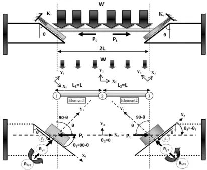
In this case study, it is assumed that there is a friction force between two faces of slant end-plates at connection. So, an elastic spring stiffness, Kg, is used instead of friction reaction in sup-ports at the local axes directions. As shown in Figure 6, the stiffness of this spring depends on the amount of friction factor and direction of sliding. Before any thermal effect, the beam is subjected only to symmetric transverse load. Therefore, the two end-plates with rollers tend to slide down-ward but the friction force that is replaced by spring, Kg, resists against sliding on the slant plane. In calculating the stiffness of spring, the displacements of the end-plate on slanting lines (X1 and X3) due to shortening of beam by initial axial load, Pi, are required.

l

L W

Pi Pi Kg

θ θ

W

θ θ

θ

Ry

θ

L =L L =L

1 2 3

Element1 Element2

Y2

X2 X1

Y1 Y3 X3

X1 Y1

X3 Y3

Y2

X2

θ =9 ‐θ θ =

θ =‐θ

Ry3

9 ‐θ 9 ‐θ

RM RM3

Kg

Ff Ff

Pi Pi

Figure 6:Force diagram of beam with slant end-plate connections due to symmetric transverse load (friction supports, before elevated temperature).

(12)

1 1 1

2 2 2

3 3 3

[

]

rotation rotation rotation g g total

dx K dx fx

dy Ry fy

d Rm fm

dx Rx fx

dy Ry fy

d Rm fm

dx K dx fx

dy Ry fy

d Rm fm

K

     



 





 





 





 





 





 





 







 





 



 



 



 



 



 





(14)

From Equation 14, it can be found that the total stiffness matrix is similar to the first case study (frictionless support). But when the friction support is used, the reaction force of spring,

Kgdxi, should be considered. After the substitution of the reaction force of spring into the reaction

vector, the displacement and initial axial force due to the symmetric transverse load before thermal effect can be obtained with the following B.C.

(15)

and the following corresponding expressions.

Elongation of beam in the X1 direction (frictionless case):

1 1 2

2

(2 ) cos

=

2 sin sin

x g

i x

P L W

A

L L L

AE E



 

   (16)

Free displacement in the X1 direction depending on friction:

1 1 1 1 (2 ) 2 g x x x f x f F f L

d   

 ₍₁₇₎

Friction force in the slanting direction:

sin cos f s s F WL



   













(18)

1 0,

dy  dr1 0,dx2 0, dr2 0,dy3 0, dr30,

1 K dxg 1,

Rx   Rx₂ 0, Ry₂ 0, Rm₂ 0,Rx3  K dxg 3,

2 0, fx  1 2 12 , WL

fm  

1 cos ,

2

WL

fx   1 sin ,

2

WL

fy   

2 . ,WL

fy   fm2 0,

3 cos ,

2

WL

fx    3 sin ,

2

WL

fy    3

2

, 12 WL

(13)

Stiffness of spring in the slanting direction:

1

sin cos sin

g

f s

x s

F A

L

K E

d



  

 













(19)

From Equation 16, the free displacement due to contraction on the slant direction at roller sup-port can be obtained. Equation 17 shows that when there is a friction force between end-plates, the amount of such displacement will be decreased. Hence, we can use a spring to replace and cover the free downward displacement where the friction force tends to resist sliding. The stiffness of spring before thermal effect can be obtained using Equations 18 and 19.

3.3.2 After Elevated Temperature

After elevated temperature, the primary length of the beam increases but two ends of the mem-ber are axially semi-restrained. Therefore, the reaction of support induces an axial force in the beam. This axial force depends on the elevated temperature and the boundary condition at the supports. The slanting direction of supports allows the end-plates to crawl upward when the amount of initial axial load due to elevated temperature, Pt, is higher than the axial force only due to symmetric transverse load and friction force on the slant surface. Here, the upward resistance force (friction) is simulated by a spring stiffness, Kt (Figure7).

l

L W Pt Pt

Kt

θ θ

W

θ θ

θ

Ry

θ

L =L L =L

1 _Element1 2 _Element2 3

Y2

X2 X1

Y1 Y3 X3

X1 Y1

X3 Y3

Y2

X2 θ =9 ‐θ θ =

θ =‐θ

Ry3

9 ‐θ 9 ‐θ

RM RM3

Kt

Ff

Ff Pt Pt

Figure 7:Force diagram of beam with slant end-plate connections due to symmetric transverse load and increase in temperature (friction support, after elevated temperature).

(14)

1 1 1

2 2 2

3 3 3

sin cos 0

[ total]

t

dx K dx fx P

dy Ry fy P

dr Rm fm

dx Rx fx

dy Ry fy

dr Rm fm

dx K dx fx

dy Ry fy

dr Rm fm

K                                                                                                 0 0 0 sin cos 0 t t P P                                (20)

With the following corresponding important parameters. Elongation of beam in the X1 direction (frictionless case):

1 1 1

x t x g x

L  L_ L_

    ₍₂₁₎

1 1

( sin 2 sin 2 ) x f x x x t t f L F f P d P        (22)

sin cos f s s F WL



  













(23)

1

sin

(sin cos ) (cos sin )

s s s f x t W

AE T WL

F d K                (24)

From Equation 20, it can be observed that the total stiffness matrix is similar to the case of

be-fore elevated temperature, but now the reaction force of spring, Ktdxi, should be considered. Also,

the amount of pure axial force due to elevated temperature should be added in terms of forces in the matrix equation. In calculating the stiffness of spring, Kt, the difference of the amount of

short-ening in the beam due to only transverse load, ΔLx1, and the amount of elongation in the beam due

to elevated temperature (Equation 21) should be obtained. From Equation 21, the free displacement

of the end-plate on slanting plane after elevated temperature, Δdx1 (Equation 22), can be computed.

(15)

3.4 The Connection with Friction Bolt Support

3.4.1 Before Elevated Temperature

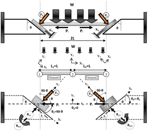
In many general end-plate connections, friction bolts are used instead of general bolts to in-crease the ability of connections due to sliding forces. By applying the tightening force, Pb, perpen-dicular to the slant end-plate, the friction force of bolts can be increased. This means there exists an additional resisting force against downward sliding when the beam is subjected to only symmetric transverse load. The total equilibrium relationship of such a beam can be expressed as:

1 1 1

2 2 2

3 3 3

[

]

g

b

g

b

total

dx K dx fx

dy Ry fy P

dr Rm fm

dx Rx fx

dy Ry fy

dr Rm fm

dx K dx fx

dy Ry fy P

dr Rm fm

K

 



 

 





 





 





 





 





 





 





 





 





 





 





 





 





 





 



(25)

with the following expressions.

1 1 2

2

(2 ) cos

=

2 sin sin

x g

i x

P L W

A

L L L

AE E



 

   (26)

1 1

(2 )

2 g x x

x f

x

f F

f L

d   

 ₍₂₇₎

( ) ( sin ) sin cos

s b

s f

F WL WL P



  

  (28)

2

1

( sin sin )

cos ( sin )

g

f s b

x s b

F AE WL P

d L P

K

WL WL

 

   

   













(29)

(16)

initiat-ing from equilibrium, Equation (25), the stiffness of simulated sprinitiat-ing, Kg, can be obtained from Equation (29).

l

θ _θ

L W

Pi Pi Kg

θ θ

W

θ θ

Ry

L =L L =L

1 2 3

Element1 Element2

Y2

X2 X1

Y1 Y3 X3

X1 Y1

X3 Y3

Y2

X2

θ =9 ‐θ θ =

θ =‐θ

Ry3

9 ‐θ 9 ‐θ

RM RM3

Kg

Ff

Pi Pi

Pb P_b

Figure 8:Force diagram of beam with slant end-plate connections due to symmetric transverse load (with friction bolts, before elevated temperature).

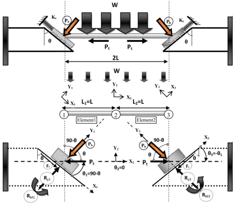
3.4.2 After Elevated Temperature

(17)

l L

W

Pt Pt

Kt

θ θ

W

θ θ θ

Ry

θ

L =L L =L

1 2 3

Element1 Element2

Y2

X2

X1

Y1 Y3 X3

X1 Y1 X3 Y3 Y2 X2

θ =9 ‐θ θ =

θ =‐θ

Ry3

9 ‐θ 9 ‐θ

RM RM3

Kt

Ff

Ff Pt Pt

Pb Pb

Pb _P_b

Figure 9:Force diagram of beam with slant end-plate connections due to symmetric transverse load and increase in temperature (with friction bolts, after elevated temperature).

1 1 1

2 2 2

3 3 3

sin [ ] b total b t t t t

dx K dx fx P

dy Ry fy P P

dr Rm fm

dx Rx fx

dy Ry fy

dr Rm fm

dx K dx fx

dy Ry fy P

dr Rm fm

K                      _                                                                           cos 0 0 0 0 sin cos 0 t t P P                                 (30)

along with the following expressions.

1 1 1

x t x g x

L  L_ L_

    ₍₃₁₎

1 1

( sin 2

(18)

( sin )

sin cos

f

s b

s

F WL WL P 

 

  

 













(33)

sin ( sin )

(sin cos ) (cos sin )

s b

s s s b

t

WL P

L

AE T WL P

K

 

   



 

       



(34)

4 EXPERIMENTAL TESTS AND COMPARISON WITH DIRECT STIFFNESS

FORMULATION RESULTS

The structural responses computed with the direct stiffness method are first validated with experi-mental results. Experiexperi-mental data was taken from small scale steel beam and frame tests carried out at the Faculty of Civil Engineering of Universiti Teknologi Malaysia (UTM). The geometrical details for the considered structure are shown in Figure 10. H sections with a thickness of 1.5 mm were employed for beam and columns. The height of columns and beam’s length of 235 mm and 450 mm were considered, respectively.

4 5 0

1 . 5

5 0

1 . 5

Figure 10:Geometrical details of the slant end-plate connection in a beam-to-column system for experimental study (all units are in mm).

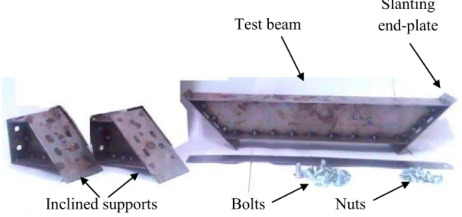
Test beam

Inclined supports Bolts Nuts

Slanting end-plate

(19)

Figure 11 shows the composition of components used in the experimental study. The structure consists of five separated parts; two columns, two short side beams and a middle beam with two inclined ends. These five parts were assembled by normal bolts and nuts. For the tests, the side beams and middle beam were detached as separate components from the main frame, resembling those of the analytical assumptions. The slant end-plate connection can damp thermal axial force by motion on slant surface, so in the experimental model, the holes on slant end-plate connection were constructed such that they are of oval shape to allow this deformation. According to direct stiffness equations, the friction factor, µs, between two faces of slant end-plate connection joint is desired. So, a basic test was conducted to determine this as shown in Figure 12. In the friction test

the self-weight of beam is measured 6.67 N with a connection slanting angle of 45° (_� = 45°).

A 39.22 N attachment weight was used on the top of side beam in the vertical position. To measure the amount of sliding force, a load cell with 50 kA- 5 kN capability was located at the side of the beam. An automated data logger (UCAM-70A) was used to measure the corresponding axial

force. The basic test measured a magnitude of 0.37 (µs = tan φ) for the static friction factor of the

inclined surfaces. After the determination of the friction factor, two additional tests; before and after elevated temperature, were carried out for measuring the structural performance of the current connection system. The test set-up can be seen in Figure 13 where the beam was tested with seven symmetric gravity load intensities (6.67 N, 26.29 N, 45.91 N, 65.53 N, 85.15 N, 104.77 and 124.39 N) including beam self-weight. Similar to the basic test, the axial force is recorded using the data logger with a load cell located at the end of the beam. For controlling the temperature under 100° (elastic zone) (EC3, 2005), ten thermocouples were attached along the beam with the heat source coming from a hot air blower placed at the middle of the beam. Note that Equations (14) and (20) from the model with the friction support assumption are specifically employed to produce the nu-merical results, to be compared to experimental responses.

Weight

Load cell

Data logger

Beam

Sketch of friction test Rigid plate

Figure 12:Basic test for finding the static friction factor (µs) between two faces of slant end-plate connection.

(20)

ac-ceptably to the outcomes produced by experiments, both before and after temperature increase, and thus validating the applicability of the current numerical method.

Thermocouple readings

Data logger

Load cell Beam

Hot air blower Transverse load

(a)

(b)

Figure 13:a) Thermal test set-up and b) method of applying temperature increase.

0 10 20 30 40 50 60 70 80 90 100 110 120 130 140 150

0 10 20 30 40 50 60 70 80 90 100 110 120 130 140

Applied symmetric load W(N)

Direct stiffness,Pi,(W)

Direct stiffness,Ptmax,(W+?T)

Experimental,Pi,(W)

Experimental,Ptmax,(W+?T)

Figure 14:The relationship between symmetric load and axial force in the beam (friction factor, μs = tan φ = 0.37, � = 45°).

A

x

i

al

force

in

the

beam

(21)

5 NUMERIC PARAMETER STUDY

After a good agreement with experimental outcomes, we demonstrate next using the model ap-proach the evaluation of the minimum requirement of initial axial force for equilibrium that initi-ates the motion at the two ends of the beam for several parametric changes. Also, the corresponding minimum elevated temperatures for end-plate crawling are computed. The structural model de-scribed in the previous section has been used to analyze a steel beam section at elevated tempera-ture, in which an I-section (build-up) beam is connected at its ends to slant fixed end-plate supports (Figure 15). For demonstration purpose we have set for the beam: cross section area (A) = 14000

mm2, modulus of elasticity (E) = 200 kN/mm2, ambient temperature (T0) = 20°C, elevated

tem-perature (ΔT) = 50°C, length of beam (L) = 6000 mm, coefficient of thermal expansion (α) = 1.5 ×

10-5 °C-1, linear symmetric transverse load (W) = 10 kN/m, and the perpendicular axial force

(tightening force) on the friction bolts (Pb) = 50 kN (total force). The slope of slant end-plate

con-nection (�) and the friction coefficient factor (μs = tan φ) are varied.

l PL 300×20

Pi

θ θ

W= kN/m

θ θ

L = m L = m

1 _Element1 2 _Element2 3

Y2

X2 X1

Y1 Y3 X3

X1 Y1

X3 Y3

Y2

X2 θ =9 ‐θ θ =

θ =‐θ

9 ‐θ 9 ‐θ

kN/m 6. m Pi

Pi

PL 200×20

Section of beam PL 200×20

Figure 15:Numerical model geometrical detail.

In addition, a two dimensional numerical finite element model is created using the commercially available software, ABAQUS, for comparison. In the ABAQUS model, the slant support compo-nents are modeled using the continuum tetrahedral brick elements and the beam is constructed using the beam element. The contacts between end-plates are simulated by the node-to-surface

for-mulation. For this illustration, we have considered four angles (� = 15˚_{, 30}˚_{, 45}˚_{, 60}˚_{) using}

three different friction factors (μs= 0.2, 0.3, 0.5). The results of one sample study where � = 30˚

and μs is 0.2 are shown in Figure 16 for 4 cases: Using general bolts and friction bolts for each case

(22)

friction bolts are used (Pi,W+Pb), the amount of axial force decreases to 18.89 kN. It is demon-strated in Figure 16 that the friction bolts can decrease the induced axial force in the beam before elevated temperature due to just symmetric transverse load. After temperature change, the

mini-mum requirement of axial force in the beam for initiation of crawling (Pi,W+ΔT) is equal to 86.54

kN, and when the friction bolt is used, the minimum requirement (Pi,W+Pb+_ΔT) is 116.46 kN,

which is higher. Also, from the results of other cases of after elevated temperature for various an-gles, it can be found that if the friction bolt is used instead of general bolts, a higher axial force is required to initiate crawling of the beam on the slant plane. The detail is shown next.

Figure 16:Schematics of ABAQUS model with arrows denoting the axial force for all considered cases for � = 30˚_andμ_{s = 0.2. Unit of forces is kN}

(23)

0 50 100 150 200 250 300 350 400 450 500 550 600 650 700

0 5 10 15 20 25 30 35 40 45 50 55 60

Ax

ia

l f

or

ce

in

th

e

beam

-c

ol

um

n

(k

N

)

Angle of inclination of slant connection

Analytical,Pi, (W) Analytical,Ptmax, (W+ΔT) Abaqus,Pi(W) Abaqus,Ptmax(W+ΔT) Direct stiffness,Pi, (W) Direct stiffness,Ptmax, (W+ΔT)

Figure 17:Relation between axial force in the beam with connection slanting (�) subjected to symmetric transverse load and elevated temperature (friction factor, μs = tan φ = 0.2, using normal bolts)

0 50 100 150 200 250 300 350 400 450 500 550 600 650 700

0 5 10 15 20 25 30 35 40 45 50 55 60

Ax

ia

l f

or

ce

in

the

be

am

-c

ol

um

n

(k

N

)

Figure 18:Relation between axial force in the beam with connection slanting (�) subjected to symmetric transverse load and elevated temperature (friction factor, μs = tan φ = 0.3, using normal bolts)

0 50 100 150 200 250 300 350 400 450 500 550 600 650 700

0 5 10 15 20 25 30 35 40 45 50 55 60

Ax

ia

l f

or

ce

in

th

e b

ea

m

-c

olu

m

n

(k

N

)

(24)

0 50 100 150 200 250 300 350 400 450 500 550 600 650 700

0 5 10 15 20 25 30 35 40 45 50 55 60

Ax ia l f or ce in th e b ea m -c olu m n (k N )

Analytical,Pi,(W+Pb) Analytical,Ptmax, (W+Pb+ΔT) Abaqus,Pi(W+Pb) Abaqus,Ptmax(W+Pb+ΔT) Direct stiffness,Pi,(W+Pb) Direct stiffness,Ptmax, (W+Pb+ΔT)

Figure 20:Relation between axial force in the beam with connection slanting (�) subjected to symmetric transverse load and elevated temperature (friction factor, μs = tan φ = 0.2, using friction bolts)

0 50 100 150 200 250 300 350 400 450 500 550 600 650 700

0 5 10 15 20 25 30 35 40 45 50 55 60

Ax ia l f or ce in the be am -c ol um n (k N )

Abaqus

Figure 21:Relation between axial force in the beam with connection slanting (�) subjected to symmetric transverse load and elevated temperature (friction factor, μs = tan φ = 0.3, using friction bolts)

0 50 100 150 200 250 300 350 400 450 500 550 600 650 700

0 5 10 15 20 25 30 35 40 45 50 55 60

Ax ia l fo rc e in th e b ea m -c ol um n (k N )

Abaqus Direct stiffness Analytical

(25)

Variation of movement initiation elevated temperatures, ΔTm, in the beam with slanting

con-nection, �, due to symmetric transverse load with normal and friction bolts, Pb, are shown in

Fig-ures 23 and 24, respectively. Again, three separate methods are used and compared. The curves of direct stiffness method match perfectly those of analytical method whereas the curves from ABAQUS model although diverge are almost parallel with them before a certain minimum inclina-tion angle, after which the agreements are excellent. Such divergence in response may be attributed to the contact behavior between 1D middle beam elements and the side-beam solid elements. Since it has been exhibited that analytical model, current numerical model and experimental results are closely matching, the divergence by the ABAQUS model can be related to non-conforming modeling setting that captures the structural response only after a certain minimum angle of slanted connec-tion inclinaconnec-tion. Between 0° to 60° of connecconnec-tion slanting, for direct stiffness and analytical

ap-proaches, if the angle of end-plate, θ, is equal to the angle of friction factor, φ, ΔTm for the beam

goes to infinity. If the slant connection’s angle, θ, is equal to 90º, tan θ, goes to infinity. As a result,

the movement-elevated temperature, ΔTm, goes to zero. This means that if the end-plate

ap-proaches the vertical position, the elevated temperature requirement for primary movement will approach infinity and if the end-plate approaches the horizontal position, the elevated temperature requirement for primary movement approaches zero. Making comparison between the amounts of

minimum elevated temperature for movement, ΔTm, it can be found that by increasing the friction

factor from zero to 0.5, the amount of minimum elevated temperature for movement, ΔTm, will be

increased. This means the friction force that resists against upward crawling at the end of beam needs higher elevated temperature to initiate movement. Also, the normal force of friction bolts can increase the friction force against upward movement of the beam, causing increase in both axial

force and ΔTm.

0 10 20 30 40 50 60 70 80 90 100

0 ˚ 5 ˚ 10 ˚ 15 ˚ 20 ˚ 25 ˚ 30 ˚ 35 ˚ 40 ˚ 45 ˚ 50 ˚ 55 ˚ 60 ˚

M

ovem

en

t

El

evat

ed

T

em

per

at

ur

e

,

ΔT

m

(

°c

)

Analytical,ΔTm,(W+ΔT ),μs=0.2

Abaqus,ΔTm,(W+ΔT),μs=0.2

Direct stiffness,ΔTm,(W+ΔT ),μs=0.2

μs

=0

.5

Practical Limitation

Maximum Elastic Modules of Steel ST37 for Ambient temperature 20˚c

ΔT = 50˚c

μs

=0

.3

D

ire

ct s

tiffn

ess

D

ire

ct s

tiffn

ess

A

nal

yti

cal

A

nal

ytical

(26)

0 10 20 30 40 50 60 70 80 90 100

0 ˚ 5 ˚ 10 ˚ 15 ˚ 20 ˚ 25 ˚ 30 ˚ 35 ˚ 40 ˚ 45 ˚ 50 ˚ 55 ˚ 60 ˚

M

ovem

en

t

El

evat

ed

T

em

per

at

ur

e

,

ΔT

m

(

°c

)

Analytical,ΔTm,(W+ΔT+Pb ),μs=0.2

Abaqus,ΔTm,(W+ΔT+Pb),μs=0.2

Direct stiffness,ΔTm,(W+ΔT+Pb ),μs=0.2

Practical Limitation

Maximum Elastic Modules of Steel ST37 for Ambient temperature 20˚c

ΔT = 50˚c

D

ire

ct s

tiffn

ess

Di

rec

t s

tiff

nes

s

Di

rect

sti

ffn

ess

A

nal

yti

cal

An

al

yti

cal

A

nal

yti

cal

Figure 24:Relation between movement initiation elevated temperature, ΔTm, and angle of slant connection subjected to symmetric transverse load and elevated temperature (in the case of friction bolts)

6 CONCLUSION

This paper reports on the development of a linear one dimensional finite element model of the steel beam with a slant end-plate connection by means of direct stiffness matrix method and ABAQUS software modeling when it is subjected to a uniform elevated temperature (under 100° C and elastic field of steel material under thermal conditions applicable to an early stage of fire incident) and a symmetric transverse load. It has been shown that the current formulation agrees excellently in terms of the elastic structural response with the conducted test results. From the comparison of results of the direct stiffness model with those of analytical, it is demonstrated that the numerical models are able to estimate practically identical amount of initial axial force and elevated tempera-ture for initiation of movement of a steel beam when a slant end-plate is used as connection. The parametric investigation shows that the thermal expansion of the restrained beam may cause higher axial force that can reduce the primary strength of the beam element. It is found that by changing connections' detail using the slant end-plate connection replacing that of vertical, the induced axial force is damped by the actions of friction sliding and movement on the slope surface of end-plate. Increase in the friction of end-plates contributes to a rise in the axial force in the beam. The use of friction bolts reduces the axial force in the beam in contrast to that using general bolts in absence of elevated temperature. It occurs conversely when the beams are exposed to elevated temperature.

From the models, it has been shown that the minimum requirement of elevated temperature for

crawling at the end of beam, ΔTm, increases when the amount of friction factor changes from zero

(27)

temperature, the friction bolts increase the friction force against upward movement of the beam,

and thus increasing ΔTm. It is notable to see that by varying the symmetric transverse load, the

friction factor, the inclination of the end-plate, and the normal force of friction bolts using the pre-sent model, we can potentially obtain the optimum design that has enough ability to absorb the huge axial force induced due to temperature increase in the beam before any yielding and buckling can occur.

NOMENCLATURE

References

AISC (2013). AISC Design Guide 27: Structural Stainless Steel. Institute of Steel Construction

Al-Jabri K.S. (2011). Modelling and simulation of beam-to-column joints at elevated temperature: A review. Journal of the Franklin Institute 348(7): 1695-1716.

Bailey C.G., Burgess I.W., Plank R.J. (1996). Analyses of the effects of cooling and fire spread on steel-framed build-ings. Fire Safety Journal 26(4): 273-293.

Bradford M. (2006). Elastic Analysis of Straight Members at Elevated Temperatures. Advances in Structural Engi-neering 9(5): 611-618.

Chen J., Young B. (2006). Stress–strain curves for stainless steel at elevated temperatures. Engineering Structures

28(2): 229-239.

Dai X.H., Wang Y.C., Bailey C.G. (2010). Numerical modelling of structural fire behaviour of restrained steel beam– column assemblies using typical joint types. Engineering Structures 32(8): 2337-2351.

EC3 (2005). Eurocode 3 (EC3), BS EN 1993-1-2: Design of Steel Structures, Part 1-2: General Rules-Structural Fire Design. . British Standards Institution London, UK.

Heidarpour A., Bradford M.A. (2009). Elastic behaviour of panel zone in steel moment resisting frames at elevated temperatures. Journal of Constructional Steel Research 65(2): 489-496.

A Cross section of beam

E Young’s modulus

Ff Friction force

I Moment of inertia

Kg Stiffness of simulated spring due to transverse

load

Kt Stiffness of simulated spring due to elevated

temperature

L Length of the beam

M Bendingmoment

Pb Totalforce of tightening in friction bolts

PcrCritical compressive axial load

A Cross section of beam

E Young’s modulus

Ff Friction force

I Moment of inertia

Kg Stiffness of simulated spring due to transverse

load

Kt Stiffness of simulated spring due to elevated

temperature

L Length of the beam

M Bendingmoment

Pb Totalforce of tightening in friction bolts

(28)

Larson S.C., Van Geem M.G. (1987). Structural thermal break systems for buildings: Feasibility study: Final report. Other Information: Portions of this document are illegible in microfiche products. Original copy available until stock is exhausted. p. Medium: X; Size: Pages: 102.

Mourão H.D.R., E Silva V.P. (2007). On the behaviour of single-span steel beams under uniform heating. Journal of the Brazilian Society of Mechanical Sciences and Engineering 29(1): 115-122.

Qian Z.H., Tan K.H., Burgess I.W. (2008). Behavior of steel beam-to-column joints at elevated temperature: Exper-imental investigation. Journal of Structural Engineering 134(5): 713-726.

Rodrigues J.P.C., Cabrita Neves I., Valente J.C. (2000). Experimental research on the critical temperature of com-pressed steel elements with restrained thermal elongation. Fire Safety Journal 35(2): 77-98.

Simões da Silva L., Santiago A., Vila Real P. (2001). A component model for the behaviour of steel joints at elevated temperatures. Journal of Constructional Steel Research 57(11): 1169-1195.

Takagi J., Deierlein G.G. (2007). Strength design criteria for steel members at elevated temperatures. Journal of Constructional Steel Research 63(8): 1036-1050.

Usmani A.S., Rotter J.M., Lamont S., Sanad A.M., Gillie M. (2001). Fundamental principles of structural behaviour under thermal effects. Fire Safety Journal 36(8): 721-744.

Yang B., Tan K.H. (2012). Numerical analyses of steel beam-column joints subjected to catenary action. Journal of Constructional Steel Research 70: 1-11.

Yin Y.Z., Wang Y.C. (2004). A numerical study of large deflection behaviour of restrained steel beams at elevated temperatures. Journal of Constructional Steel Research 60(7): 1029-1047.

Zahmatkesh F., Osman M.H., Talebi E. (2014a). Thermal Behaviour of Beams with Slant End-Plate Connection Subjected to Nonsymmetric Gravity Load. The Scientific World Journal 2014.

Zahmatkesh F., Osman M.H., Talebi E., Kueh A.B.H. (2014b). Analytical study of slant end-plate connection sub-jected to elevated temperatures. Steel and Composite Structures 17(1): 47-67.