Brazilian Journal of Physics, vol. 36, no. 3A, September, 2006 627
Polymer Dynamics: Long Time Simulations and Topological Constraints
Kurt Kremer
Max-Planck-Institut für Polymerforschung, Postfach 3148, D-55021 Mainz, Germany
Received on 2 October, 2005
Topological constraints, entanglements, dominate the viscoelastic behavior of high molecular weight poly-meric liquids. To give a microscopic foundation of the phenomenological tube, recently a method for identifying the so called primitive path mesh that characterizes the microscopic topological state of (computer generated) conformations of long-chain polymer networks, melts and solutions was introduced. Here we give a short account of this approach and compare this to long time simulations.
Keywords: Polymer dynamics; Long time simulation; Long-chain polymer networks
I. INTRODUCTION
The viscoelastic properties of polymer liquids and their link to the microscopic structure and dynamics are key issues in modern polymer science and biophysics [1–6]. For this a pro-totypical system is a melt or semi-dilute solution of long (flex-ible) chain molecules. On a microscopic scale, their Brown-ian motion is dominated by the restriction that the chains may slide past but not through each other. This introduces mo-tion constraints in a way that each polymer chain can only move along a tube like region around a so called primitive path. This primitive path is the backbone of the appropriately coarse grained chain contour [7, 8]. Recent, more refined ana-lytical [3, 9] and numerical models [10–14] concentrate on the dynamics of these primitive paths. These models are able to quantitatively describe many rheological and single chain dy-namics data with a small set of material-specific parameters such as the tube diameter,dT. It is the purpose of the present short contribution, to compare a topological approach to de-termine the tube diameter from chain conformations with long time simulations, which essentially follow an analysis close to experiments.
II. EXPERIMENTS/SIMULATIONS
The key quantity of the theory, the mesh of primitive paths or equivalently the tubes with diameterdT2∼Ne, the entangle-ment molecular weight, is experientangle-mentally not directly accessi-ble. Thus a variety of experiments have been devised, leading to estimates ofdT(or equivalently,Ne), based on different the-oretical approximations. Here we discuss three examples.
A. Chain DiffusionD(N)
The diffusion of individual beads as well as of the whole chain can be studied by a variety of experiments as well as computer simulations. Within the concept of the tube or rep-tation model one expects for the diffusion constant of a whole chain in a melt or semidilute solutions of identical other chains (Nbeing the chain length):
0.01 0.1 1
0.1 1 10 100
D
(
n
)/
DR
(
n
)
n/ne
slope −1 experimental simulation BPA−PC
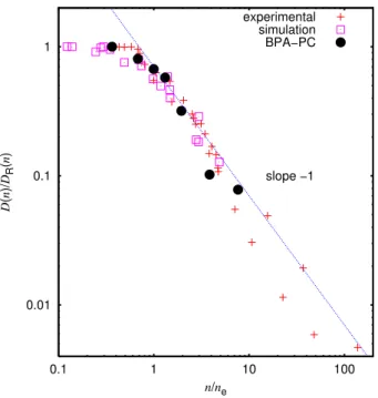
FIG. 1: Scaled diffusion constantDD(n)
R(n) for BPA-PC data and
D(N)
DR(N)
for the reference data as a function of the scaled chain lengthnn
e and
N
Ne respectively from different experimental and simulation results
for various polymer systems. The best fit for the entanglement length yieldsne=62±8 coarse grained beads, giving approximatelyNe,D≃
15. Figure taken from[16]
D(N) ∼ ½
N−1 ;N≤Ne
NeN−2 ;N≫Ne
(1)
Recent experiments even suggest a somewhat stronger de-cay for longer chains[15]. Taking the above relation, we ex-pect a universal curve, when plotting the ratio ofD(N)over the hypothetical short chain diffusion constant of the same chain length vsN/Ne. Using this one can fit a value forNe,
628 Kurt Kremer
B. Dynamic Structure Function S(q,t)
Alternatively one can also analyze the dynamic coherent scattering function of individual chains as done for example in neutron scattering experiments. For simple computer poly-mers, all form factors of the monomers or beads are taken equal and are set to one. ThenS(k,t)reads
S(k,t) = 1
N
∑
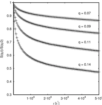
i,jexp[ik(ri(t)−rj(0))], (2) withri(t) being the position of bead iat timet. For times larger than the time a bead needs to explore the diamter of the tube, but much shorter than the time the chain needs to diffuse out of the tube, the scatterer observes a smeared out bead density within the tube, akin to the effect described by the Debye-Waller factor in solid state physics. This leads in the aforementioned time regime to a plateau in the decay of S(k,t)[17–19]S(k,t) S(k,0)={
£
1−exp[−(kdT/6)2]¤
f³k2b2p12W t/π´
+exp[−(kdT/6)2]} 8
π2 ∞
∑
p=1,oddexp[−t p2/τd]
p2 , (3)
where f(u) =exp[u2/36]er f c(u/6),bis the bond length and W is the bead friction. Figure ??shows this, again for the ex-ample of polycarbonates[16]. From the above expressiondT can be estimated. Again,dT is used to fit the data to the the-ory. If we assume thatdT2=R2(Ne) =Nec∞b2,R2(Ne)being the mean square end to end distance of a chain ofNe beads andc∞the Flory characteristic ratio [20], it is then possible to calculate the entanglement lengthNe.
C. Plateau ModulusG0N
The third approach goes back to the very origin of the tube models and employs the analogy between long chain poly-mer melts and networks. Under elongational or shear strain the initial stress relaxes rapidly towards a plateauG0N. In a simulation, the normal stressσncan be determined by the mi-croscopic virial tensor and the resulting stress plateau can be fitted to the stress strain formulas from classical rubber elas-ticity (CRE) (e.g. elongational strain in the limit of small de-formationλ) [21, 22]
σn=G(λ2− 1
λ), (4)
to determineG0N, which in turn is related toNe [1, 3] by the expression
G0N=4 5
ρkBT Ne
. (5)
0.3 0.4 0.5 0.6 0.7 0.8 0.9 1
1·104 2·104 3·104 4·104 5·104
S(q,t)/S(q,0)
t [τ*]
q = 0.07
q = 0.09
q = 0.11
q = 0.14
FIG. 2: Scaled dynamic structure factorS(q,t)/S(q,0)as a function of time for the polycarbonate melt with chain lengthN= 120 repeat units. For eachq-value, dotted lines show the fit to the expression of equation 3. Figure taken from[16]
TABLE I: Values obtained forNeusing the different approaches
dis-cussed in the text for fully flexible bead spring chains [17] and a coarse grained model of polycarbonate (BPA-PC) [16, 30]. The max-imum chain lengths studied are also indicated.
NeBPA−PC N
bead−spring e
D(N) ≈15 ≈70 S(q,t) 10 55
G0N 5-6 72
Nmax 120 2000
whereρis the bead density. This is the most direct experi-mental way to determinedT andNerespectively, as no fitting
is required and only the underlying theory is applied. How-ever, this again is not a direct measurement ofNe.
In Table I the outcome of the different approaches from simulations of a special coarse grained model of polycarbon-ate and for highly flexible simple bead spring chains are given. For both cases the material specific quantityNe is very
dif-ferent, if obtained by different methods. While this by itself is not surprising and problematic, it is the fact that the ratio of the estimates from individual "experiments" is very differ-ent for the two differdiffer-ent cases. Thus there is a clear need for an independent ansatz to obtain the material specific quantitiy Ne, without referring to the rather indirect experimental
Brazilian Journal of Physics, vol. 36, no. 3A, September, 2006 629
III. PRIMITIVE PATH ANALYSIS
To do this, we go back to the original idea of Edwards [23] who identified the random walk-like axis of the tube with what he called the “primitive” path: the shortest path between the endpoints of the original chain into which its contour can be contracted without crossing any obstacle. Similar to the tube, the primitive path is usually discussed without specifying the relation between the obstacles and the melt structure. How-ever the obstacles themselves are chains, which has to be taken into account, when constructing the primitive path [24–26]. In Ref. [24] we introduced aprimitive path analysis(PPA) where all polymers in the system are contracted simultaneously in a way, that a linear stress strain relationship is kept. This allows us to establish the microscopic foundations of the tube model and to endow a highly successful phenomenological model with predictive power for structure-property relations.
We performed the primitive path analysis on a variety of different simple bead spring chain melts [27] and semi di-lute solutions [28] with variable intrinsic stiffness [29]. All these cases include the crucial ingredients characteristic for polymeric systems: connectivity, flexibility, local liquid-like monomer packing and mutual uncrossability of the chain backbones. The parameters used for the PPA are given in [25]. Monodisperse polymer melts ofM=200−500 chains of length 50≤N≤700 at a bead density ofρ=0.85σ−3(in Lennard Jones units) are studied. By introducing a small in-trinsic bond bending potential, the Kuhn length,lK=hR2i/L, is varied between 1.80σand 3.34σ.hR2iis the mean squared end to end distance of the chain and Lis the chain contour length. For details see Ref. [29]. In addition, we present results for a coarse-grained model for polycarbonate (BPA-PC)[16, 30]. In this case, we analyzed melt configurations for M=100 chains of N=60 chemical repeat units which are represented by four beads each. All the melt samples studied are tabulated in [25].
The implementation of the PPA is straightforward: First the chain-ends are fixed in space. Then, all intrachain inter-actions other than the FENE bond interaction, which has its minimum atr=0, are switched off. Finally the total energy is minimized by cooling the system slowly toT →0. With-out thermal fluctuations and intra-chain EV interactions, the bond springs try to reduce the bond length to zero and pull the chains taut. The interchain EV interactions provide an energy barrier to prevent chain crossings. Needless to say, a crucial ingredient for the success of the whole procedure is the avail-ability of well equilibrated conformations[29, 31]! For details of the PPA protocol we refer to [25]. The algorithm intro-duced so far does not account for self-entanglements. In a recent variant of the approach this is included in the PPA [25].
IV. RESULTS - COMPARISON TO EXPERIMENTS
In order to understand the relationship between the melt structure and properties like the plateau modulus for many different polymers and simple model systems we need a di-mensionless way to compare data. To render theG0
N values
dimensionless, we need an energy scale and a length scale. As the dominant contribution toG0Nis of entropic origin,kBT as the energy scale suggests itself. However, there are essen-tially two independent length scales that characterize the local structure of polymer melts. One, the Kuhn length,lK [1] is defined for random walks as the length of an individual step of a freely jointed chain with the same mean-square end-to-end distancehR2i=l
KLand contour lengthL. Random walks however do not densely fill space. Locally however, most monomers will belong to the same chain. The length at which the polymers start to interpenetrate is given by the packing length,p= (ρchainhR2i)−1. The packing length can be visual-ized as the average strand strand distance. It is relevant to note that the product of the number density of chains,ρchain, and of
hR2iis independent of chain length for a fixed monomer num-ber density,ρ. Following the standard convention [32] based on the chemical structure of the polymers, we chooselKas the unit of length. With this choice, instead ofG0Nwe can consider the dimensionless quantityG0Nl3K/kBT. This quantity has to be a function of the only remaining dimensionless parameter: the ratio of Kuhn and packing lengthlK/p.
The available experimental data for dense melts are the re-sult of a long term substantial experimental effort [33, 34]. Rheological measurements were performed on these sam-ples and in many cases thehR2ivalues were determined us-ing small angle neutron scatterus-ing. Refs. [33, 34] provide the values for the plateau modulus, G0N, the mass density,
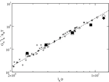
ρm, the ratio of the mean-square end-to-end distance to the molecular weight of the polymer, hR2i/M, and the packing length,p=M/(hR2iρmNA), whereNAis the Avagadro num-ber. All the melt data points obey the empirical relation G0N =0.00226kBT/p3, indicated as the dashed line in Fig. 3. The way to determinelk for experimental systems, depends on the definition of the contour length. It is however worth-while to note, if the empirical relation is valid, then any choice forlK will preserve the scaling relationship betweenG0N and p. The actual choice forlK will determine the position of the data points in Fig. 3 and will just move them along the dashed line in the figure. All the melt data shown in the figure are tabulated in [25], where also a more detailed discussion of the mapping and the length scales can be found.
The aforementioned mapping can be also be used to identify bead spring polymer models to individual chemical species. The standard model [27] with fully flexible polymer chains used in molecular dynamics simulations corresponds tolK/p=2.68. Among the available experimental data, the chemical species with the closestlK/pvalue is natural rubber (cis-Polyisoprene) withlK/p=2.72. This suggests that the elastic properties of the usually studied bead spring polymer model corresponds most closely to that of natural rubber, the prototypical experimental system for elastic behavior.
V. DISCUSSION
630 Kurt Kremer
2×100 1×101 lK/p
10-2 10-1 100 101
GN
0 lK
3 /k
B
T
FIG. 3: Dimensionless plateau moduliG0NlK3/kBT as a function of
the dimensionless ratiolK/pof Kuhn lengthlKand packing length
p. Inset (a) contains (i) experimentally measured plateau moduli for polymer melts[? ] (∗Polyolefins,× Polydienes, + Polyacrylates and⊲miscellaneous, (ii) plateau moduli inferred from the normal tensions measured in computer simulation of bead-spring melts [17, 24] (¤) and a semi-atomistic polycarbonate melt [16] (♦) under an elongational strain, and (iii) predictions of the tube model Eq. 6 based on the results of our PPA for bead-spring melts (¥), and the semi-atomistic polycarbonate melt (¨). The line indicates the best fit to the experimental melt data for polymer melts by Fetterset al.[34]. Errors for all the simulation data are smaller than the symbol size.
To this end, we use the standard expression [1, 24]
G0N=4 5
kBT
p dT2 = 4 5
ρkBT
Ne
, (6)
which relates the plateau modulus to the Kuhn length of the primitive path. ThedT values can be obtained from the
con-tour length of the primitive path,Lpp(which is the sum of the
lengths of all the back bone bonds of a chain averaged over all the chains in the melt) usingdT=hR2i/Lpp. For details refer
[24, 25]. Fig. 3 shows an explicit comparison of the dimen-sionless plateau moduli G0NlK3/kBT of experimental systems
and bead-spring model polymers with identical ratios lK/p.
The good agreement of the two data sets confirms the insensi-tivity of entanglement effects to atomistic details and provides the necessary validation of our generic bead-spring models.
VI. ACKNOWLEDGEMENTS
The present results are a subset of those, which are originat-ing from a very fruitful and (in some cases) very longstandoriginat-ing collaboration with G. S. Grest, R. Everaers, S. Sukumaran, C. Svaneborg, L. Delle Site and S. Leon. The present work is updated and shortened version of Ref. [35].
[1] M. Doi and S. F. Edwards, Theory of Polymer Dynamics, Clarendon: Oxford 1986.
[2] H. Watanabe, Prog. Pol. Sci.24, 1253 (1999). [3] T. C. B. McLeish, Adv. Phys. bf 5, 1379 (2002).
[4] D. Humphrey, C. Duggan, D. Smith, and J. Käs, Nature416, 413 (2002).
[5] T. T. Perkins, D. E. Smith, and S. Chu, Science264, 819 (1994). [6] R. B. Bird, R. C. Armstrong, and O. Hassager, Dynamics of
Polymeric Liquids, Vol. 1, Wiley: New York (1977). [7] S. F. Edwards, Proc. Phys. Soc.92, 9 (1967). [8] P. G. J. de Gennes, J. Chem. Phys.55, 572 (1971).
[9] A. E. Likhtman, T. C. B. McLeish, Macromolecules356332 (2002).
[10] Y. Masubuchi, J.-I. Takimoto, K. Koyama, G. Ianniruberto, G. Marrucci, and F. Greco, J. Chem. Phys.1154387 (2001). [11] J. T. Padding, W. J. Briels, J. Chem Phys.117, 925 (2002). [12] K. Iwata, M. Tanaka, N. Mita, and Y. Kohno, Polymer43, 6595
(2002).
[13] M. Doi, J. Takimoto, Phil. Trans. R. Soc. Lond. A361, 641 (2003).
[14] J. D. Schieber, J. Neergaard, and S. Gupta, J. Rheol.47, 213 (2003).
[15] T. P. Lodge, Phys. Rev. Lett.83, 3218 (1999).
[16] S. Leon, L. D. Site, N. van der Vegt, and K. Kremer, Macro-molecules38, 8078 (2005).
[17] M. Puetz, K. Kremer, and G. S. Grest, Europhys. Lett.49, 735 (2000).
[18] P. G. de Gennes, J. Phys. (Paris)42, 735 (1981).
[19] P. Schleger, B. Farago, C. Lartigue, A. Kollmar, and D. Richter,
Phys. Rev. Lett.81, 124 (1998).
[20] P. Flory, Statistical Mechanics of Chain Molecules, Inter-science: New York (1969).
[21] L. R. G. Treloar,The Physics of Rubber Elasticity, Clarendon Press: Oxford (1975).
[22] J. D. Ferry,Viscoelastic Properties of Polimers, Wiley: New York (1980).
[23] S. F. Edwards, Brit. Polym. J.9, 140 (1977).
[24] R. Everaers, S. K. Sukumaran, G. S. Grest, C. Svaneborg, A. Sivasubramanian, and K. Kremer, Science303, 823 (2004). [25] S. K. Sukumaran, G. S. Grest, K. Kremer, and R. Everaers, J.
Polym. Sci. Part B: Polym. Phys. Ed., to be published (2004) [26] M. Rubinstein, E. Helfand, J. Chem. Phys.82, 2477 (1985). [27] K. Kremer, G. S. Grest, J. Chem. Phys.92, 5057 (1990). [28] P. Ahlrichs, R. Everaers, B. Duenweg, Phys. Rev. E64, 040501
(2001).
[29] R. Auhl, R. Everaers, G. S. Grest, K. Kremer, and S. J. Plimp-ton, J. Chem. Phys.119, 12718 (2003).
[30] C. F. Abrams, K. Kremer, Macromolecules36, 260 (2003). [31] R. S. Hoy, M. O. Robbins, Phys. Rev. E72, 061802 (2005). [32] W. W. Graessley, S. F. Edwards, Polymer22, 1329 (1981). [33] L. J. Fetters, D. J. Lohse, D. Richter, T. A. Witten, and A. Zirkel,
Macromolecules27, 4639 (1994).
[34] J. Fetters, L. D. Johse, and W. W. Graessley, J. Polym. Sci. B: Polymer Phys.37, 1023 (1999).