Lat. Am. j. solids struct. vol.12 número5

(1)

Abstract

The application of gradient-based methods to structural optimiza-tion problems usually requires the determinaoptimiza-tion of displacement sensitivities with respect to design variables. In this regard, it is important to have at hand comprehensive methods for sensitivity analysis, which show stability, efficiency and accuracy. Particular-ly, application of the semi-analytical method for linear and nonlin-ear problems is generally a good trade-off between formulation simplicity and accuracy. In spite of that, semi-analytical methods are known to behave pathologically for shape design variables when the structure is subjected to rigid rotations. A large number of solutions for this problem have been presented in last years, although the formulation involved is generally not trivial, especial-ly in the nonlinear case. A recent method, which adopts the semi-analytical approach and uses complex variables has rendered very promising results for all the aforementioned aspects: stability, efficiency and accuracy. Additionally, it is simple to codify. The present contribution is concerned with the application of this sensitivity analysis method to geometrically nonlinear truss prob-lems. To this end, a finite element formulation is presented and displacement sensitivities are evaluated with respect to material and shape design variables. The results are compared to those obtained using the semi-analytical method with real variables and to global finite differences. An example demonstrates the potenti-ality of this new approach.

Keywords

Structural optimization, Sensitivity analysis, Finite element meth-od, Nonlinear analyses.

Application of the Complex Variable Semi-analytical

Method for Improved Displacement Sensitivity

Evaluation in Geometrically Nonlinear Truss Problems

Geovane Augusto Haveroth a Joânesson Stahlschmidt b Pablo Andrés Muñoz-Rojas c Departamento de Eng. Mecânica, Universidade do Estado de Santa

Catarina, UDESC, Campus Univ. Avelino Marcante, CEP 90226-100, Joinville, SC, Brazil

a_{geovaneah@gmail.com} b_{joanesson@ibest.com.br} c_{pablo@joinville.udesc.br}

http://dx.doi.org/10.1590/1679-78251911

(2)

Latin A m erican Journal of Solids and Structures 12 (2015) 980-1005

1 INTRODUCTION

Sensitivity analysis is concerned with the evaluation of gradients of a structural response with re-spect to design variables. The response of interest may be the field of displacements, stresses or strains, a natural frequency, a bucking load, and so on. Typical design variables are shape or mate-rial parameters, which can be modified in the design stage, such that their change affects the overall behavior of the structure (Kleiber et al., 1997). Many methods have been developed to accomplish the sensitivity evaluation task, and for linear problems, a high level of maturity has already been achieved. This is not exactly the situation in problems that involve some kind of nonlinearity, and an important research field is still open in this case (Choi and Kim, 2005).

Methods for sensitivity analysis can be classified into three different groups: analytical methods, semi-analytical methods and overall finite differences. It is important to remark that the use of the traditional semi-analytical method for the evaluation of sensitivities with respect to shape design variables can provide unacceptable errors when the structure suffers large rigid body rotations, as reported in a large number of publications. In the case of linear problems, this pathology has been the subject of studies by Barthelemy et al. (1988), Pedersen et al. (1989), Cheng and Olhoff (1991), Mlejnek (1992), Olhoff et al. (1993), Keulen et al. (2005), Bletzinger et al. (2007), and many more. De Boer and Keulen (2000) and Parente and Vaz (2001), among others have proposed some reme-dies for the drawback in the case of nonlinear problems.

Recently, a modification of the semi-analytical method introducing the use of complex variables has been successfully applied to solve the mentioned pitfall (Jin, 2008; Jin et al., 2009; Jin et al., 2010). Their study dealt with linear and a few nonlinear heat, beam and plate problems, and showed accuracy as well as efficiency, since only a marginal extra computational cost is required. An important feature of the method is that it allows extremely small numerical perturbations with-out compromising accuracy.

The present article aims to show how the semi-analytical complex variable sensitivity analysis method behaves when applied to geometrically non-linear truss problems. To this end, the corre-sponding nonlinear finite element formulation is developed and detailed. Here it is important to remark that nonlinear sensitivity analysis requires the use of the exact tangent stiffness matrix, as will be shown. Displacement sensitivities with respect to material and shape design variables are studied in a problem dominated by rigid rotations. Results are compared to the semi-analytical method using real variables and to overall finite differences. For conciseness, the following acronyms are used throughout the text: CVSA (Complex Variable Semi-Analytical), RVSA (Real Variable Semi-Analytical), FFD (Forward Finite Difference), CFD (Central Finite Difference) and OFD (Overall Finite Difference). In this work, the CVSA method is always based on FFD.

2 GEOMETRICALLY NONLINEAR FINITE ELEMENT FORMULATION FOR TRUSSES

(3)

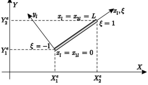
In Fig. 1, a typical 2 noded truss element is displayed, and 2 associated systems of reference are

defined: a still, global system of reference

XY

and a corotational local system of reference x y_{l l}

.

A

parametric coordinate is also defined along the length of the bar.

Figure 1: Bar finite element.

The local coordinates and displacements of any given point in the undeformed element are obtained applying a linear interpolation of the nodal values, i.e.,

( )

l l

X N X and u_l N( )u_l, (1-2)

so that at any time, the updated rotated bar geometry can be expressed by

( )

l l l l

x X u N x (3)

where

1 2

( ) N ( ) 0 0 N ( ) 0 0

N , (4)

1 1 1 2 2 2

T

l X Y Z X Y Z

X , (5)

1 1 1 2 2 2

T l ux l uy l uz l ux l uy l uz l

u (6)

and

1 1 1 2 2 2

T l xl yl zl x l yl z l

x , (7)

with N₁and N₂ being the linear interpolation functions

1 1 ( )

2

N and ₂( ) 1

2

N . (8-9)

Additionally, using (1) and (3), the corresponding Jacobians are expressed by

( )

2

l o

l

dX L

J X

d and ( ) 2

l l

dx L J x

d , (10-11)

(4)

In a nonlinear FE formulation, at each n-th load step, equilibrium must be satisfied. Thus,

min-imization of the residual R_n(difference between external and internal forces) is sought for, that is,

( )

n n n 0

R p f u , (12)

wheref is the global internal force vector, n stands for the load step and is a parameter that

controls the percentage of the total global external load vector p applied at the n-th step. The

ab-sence of subscripts

l

indicates that the equations are set in the global system of reference

(compo-nents in

X

and

Y

directions).

Taking the exact linearization of (12) by means of a Taylor series expansion truncated at first

order terms with origin at u_n , results in

1

n n

n n n n n n n n

n

d

0

R u

R u R u u R u u

u , (13)

where stands for the iteration number.

Starting at a prescribed arbitrary initial point 0

n

u

1)

, which in general does not satisfy

equilibrium, (13) must be solved iteratively until the residual falls into a prescribed tolerance range

(the tilde indicates that the value is not converged). The determination of unrequires the

evalua-tion of the residual derivative with respect to u_n . This derivative is called stiffness tangent

ma-trix and is obtained by differentiation of the external and internal force vectors. Aiming at the evaluation of (12) and (13), the expressions of the internal force vector and tangent matrix are de-rived in the remainder of this Section.

2.1 Virtual Work

One traditional manner to set up the conditions that grant equilibrium to a deformable body is the application of the Principle of Virtual Work. This principle states that the work performed by a real external force applied on a point of the body, over an imaginary (virtual) and arbitrary

dis-placement of the point ( W_ext), must equal the work performed by internal forces in equilibrium

with the real force applied, over the displacement field in equilibrium with the prescribed virtual external displacement.

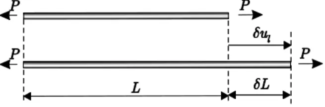
The expression for the virtual work resultant from a virtual displacement on a bar that is

al-ready subjected to a force P is easily developed, as seen in Fig. 2.

Figure 2: External virtual work.

)

(5)

While the external work ( W_ext) acting on the bar in Fig. 2 is given by

ext l

W P u , (14)

the internal virtual work Wi can be expressed using different stress and strain definitions, provided

that their joint use leads to the same virtual work given by Wext. Stress and strain measures that

satisfy this condition are said to be energetically or work conjugate. The rotated engineering stress

and engineering strain measures are defined as1

0

E

F

A and E

l l

l

dx dX

dX . (15-16)

Using (10) and (11), it turns out that

E

l l o l

l o o

J x J X L L u

J X L L , (17)

where a linear displacement profile is assumed. Therefore, the virtual strain resulting from a virtual displacement is

1 E

E l l

l o

d

u u

du L , (18)

and the following identities hold

ext l l o l E o l E E o o i

o

P

W P u A u A u A u A L W

A , (19)

where is the rotated Cauchy stress measure, and A_o and A are the undeformed and deformed

areas of the cross section, respectively.

In (19) it is implicit that the stress value is the same along the length of the bar. Generalization leads to

o

i _V E E o

W dV , (20)

and the rotated engineering stress and strain pair is shown to be work conjugate. In this derivation, a given entity is said to be rotated if it is referred to the corotational system of reference.

1_I_{n bar structural elements, out of all the}_{components of the stress tensor, only}

11 xl is not null and

produc-es work. Thus, in this text, the scalar strproduc-ess measurproduc-es cited are always the component _xl of the respective stress tensors. The same applies for the strain tensors.

( )

(6)

2.2 Internal Force Vector

Generalizing the derivation presented in Section 2.1 to a truss structure, the use of (1) and (2) leads to the discretized version of the principle of virtual work

1 1 o

ext

i i

nel nel

T T

ext l l _V E E o

e e

W

W W

W u f dV u p, (21)

where e stands for a given element,

nel

is the total number of elements and Wext now stands for

the virtual work caused by the virtual displacement u . The fl vector contains the components of

the element nodal internal force with respect to the local system of reference andp is a vector

con-taining the external applied loads with components referenced to the global system of reference. In

the particular situation shown in Fig. 2 and equation (14), p P 0 0 0 0 0T.

For a given element e

,

from (17) one has

1 E l l l l dJ x

J X du u , (22)

and noting that (22) is valid for an arbitrary u_l, after some manipulations, it results

1

T

l o EJ X A dl o

f B , (23)

where

1

1 0 0 1 0 0 2

o

l

J X

B . (24)

In order to map the internal force vector to the global system of reference used in (12), the rotation

matrix

T

is employed, leading to

e T

l

f T f , (25)

where the upperscript e in _fe_{indicates that the element vector has its coordinates refered to the}

global system of reference,

0

T _and

1 1 1

2 2 2

3 3 3

l m n

l m n l m n

. (26-27)

In (26) and (27), l_i, m_i and n_iare the direction cosines of the orthogonal local axes of the bar with

respect to the i-th global axis. In practice, noting that in (24) just the first and the fourth matrix

components are nonzero, only l₁, m₁and n₁need to be computed.

( )

(7)

2.3 Tangent Stiffness Matrix

From (13), the tangent stiffness matrix is calculated by differentiation of the residual with respect to the displacement vector set in the global reference system. If the external force vector is constant at each load step, the tangent matrix for each element is given by

e

T

T _e _e l

d d

f

k T f

u u , (28)

where

_u

e _{is the element nodal displacement vector with respect to the global reference system.}

Dif-ferentiation of (25) yields

1 2

T T

T

T l

T _e l _e

d d d d k k f T

k f T

u u . (29)

After some algebra, the term kT₁ can be expressed as (Stahlschmidt, 2013)

1

1 1

T

T J X dl

k B HB , (30)

where

1 0 0 1 0 0

1

0 1 0 0 1 0

2

0 0 1 0 0 1

l J X

B _, ₍₃₁₎

2 1

E oA e eT T

H I Bx x B _, ₍₃₂₎

0 /

L L is the stretch ratio,

I

is the identity matrix of order 3, and x contains the nodal

coor-dinates with respect to the global system of reference.

The term k_T₂ of Eq. (29) can be developed and arranged as

1

2 2

1

T T T

T oE oJ X dl T l

k T B B T = T k T. (33)

The global tangent stiffness K_T is obtained applying an assembly operator

1

nel

e which maps local to

global degrees of freedom and sums the contribution of each element to the stiffness (or force vec-tors) of the whole structure (Hughes, 1986), i.e.

1 2

1 1

nel nel

T T T T

e e

K k k k . (34)

( )

(8)

It is important to remark that in linear analyses, the term k_T₁vanishes and the linear equation (13)

is exact, so the whole load can be applied in just one step ( ₁ 1), 0

1 0

u and 0

1( 1 0) 0

R u .

Thus, the discretized equilibrium (13) particularizes to

1 0

1 1 ( )1

R u u p f u (35)

1 0

1 1 1 1 0

R u u R u

0 1 1 0 1 d d 0 R u u

u , (36)

or

p = Ku, (37)

where 2 1 nel T e

K k

,

1

nel e

e

p p

and

1

nel e

e

f f

.

(38-40)

3 SENSITIVITY ANALYSIS METHODS

A brief review of the main aspects of each of the sensitivity methods considered in this work is giv-en in this Section.

3.1 Methods Based on Real Variables

Overall (Global) Finite Difference Method

In linear problems, the displacement sensitivity can be approximated using forward finite differences by running the FEM code independently for unperturbed and perturbed design variables and per-forming a finite difference between the displacements obtained, i.e.,

( ) ( )

( ) j ( )

j j j _FFD

d

ds s s

u s s u s

u s u s

, (41)

where s represents the design variables vector and sjis a perturbation in the j-th design variable

0 0 0T

j sj

s . (42)

Similarly, central finite differences are calculated by

( ) ( )

( )

2

j j

j _CFD j

s s

u s s u s s u s

. (43)

( )

(9)

In nonlinear problems, the calculation of the finite difference sensitivity follows the same procedure,

except that displacements are evaluated at the n-th load step using (13) and

1 n

n i

i

u u _. ₍₄₄₎

Equations (41) and (43) are replaced by

( ) ( )

( ) n j n

n

j _FFD j

s

s s

u s u s

u s (45) and ( ) ( ) ( ) 2

n j n j

n

j _CFD j

s s

u s u s u s

,

(46)

where the absence of the tilde over the displacement vector u_n indicates that the converged value

for the n-th load step is used in the computation.

Semi-Analytical Method

In the linear case, displacement sensitivity is obtained by differentiation of (37) with respect to the

design variable s_j, which leads to

1

( ) ( ) ( )

( )

j j j

d d d

ds ds ds

u s p s K s

K u s _. ₍₄₇₎

Evaluating the derivatives in the RHS exactly, leads to the so-called analytical method. On the other hand, if the same derivatives are approximated via finite differences, the semi-analytical sensi-tivity expression below is obtained

1

( ) ( ) ( )

( )

j j j

d

ds s s

u s p s K s

K u s _. ₍₄₈₎

Similarly, in the nonlinear case, the residual given by (13) is differentiated. If the derivatives in the

RHS with respect to the design variable s_j are calculated exactly, the analytical method results. On

the other hand, if the same derivatives are approximated via finite differences, the semi-analytical expression is obtained

1 ( , ) 1 ( , ) _{( )}

n n n n n n

T T n

j j j j

d

ds s s s

u R u s f u s p s

K

( )

K _. ₍₄₉₎

(10)

An important aspect to be observed is that the algebraic system given by Eq. (49) is linear. As there are no iterations to correct any inaccuracy in the solution, the use of the exact tangent matrix is mandatory. This is the reason that motivated the previous presentation of Section 2.3.

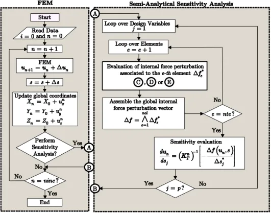
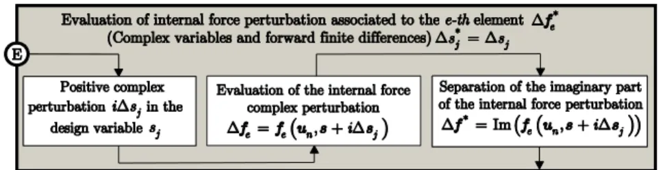
The numerical implementation of the semi-analytical procedure using both forward and central finite differences is shown in Figs. 3 and 4.

3.2 Methods Based on Complex Variables

A method for the evaluation of derivatives employing complex variables was developed in the 70s (Lyness and Moler, 1967), and has been increasingly explored in several areas of engineering (New-man III et al., 1998; Martins et al., 2000; Burg and New(New-man III., 2001; Kawamoto et al., 2005; Mundstock and Marczak, 2009; Jin et al., 2009; Jin et al., 2010; Montoya et al., 2015). The method is extremely accurate, since when double-precision complex numbers are used, the smallest non-zero

number that can be represented is 10-308 (Martins et al., 2000). It is also a promising alternative to

deal with drawbacks present in finite differences and in the semi-analytical method based on real variables.

Figure 3: Calculation of displacement sensitivities via the semi-analytical method. Particularization for real or com-plex variables depends on the procedure that evaluates the internal force variation at the element level ( *

e

(11)

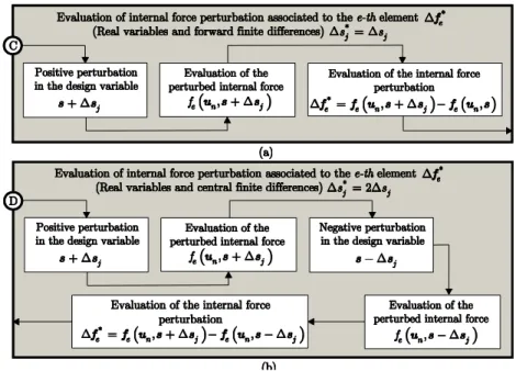
Figure 4: Details of the procedure adopted to evaluate the internal force variation (highlighted block in Fig. 3), in case of the RVSA method: (a) using FFD and (b) using CFD.

Global Finite Difference Method with Complex Variables

Following Lyness and Moler (1967) apud Mundstock (2006), the first derivative of a function

f s

( )

can be calculated by simple evaluation of the imaginary part of the perturbed function in a given

point. To show this, let us expand the function

f s

( )

using a Taylor series,

2 3

''( ) '''( )

( ) ( ) '( ) ...

2 6

f s s f s s

f s s f s f s s (50)

Now, if instead of introducing the real perturbation s, this is replaced by an imaginary

counter-part i s, the Taylor expansion gets the form

2 3

''( )( ) '''( )( )

( ) ( ) '( ) ...

2 6

f s i s f s i s

f s i s f s f s i s (51)

Using the fact that

_i

2

₁

_{, the imaginary part of the Eq. (51) is}

3 '''( )

Im ( ) '( ) ...

6

f s s

f s i s f s s (52)

and the first order derivative of

f s

( )

is given by

2

Im ( )

'( ) f s i s ( )

f s O s

(12)

It is important to observe that the sensitivity approximation given by (53) does not involve sub-traction between two different (and close) values, a fact that produces error in the traditional finite difference method. Moreover, the remainder of the approximation in (53) is of order 2, while the traditional finite difference counterpart provides approximation of order 1. Approximation of order 2 means that the sensitivity converges quadratically with a decrease in the perturbation (Martins et al., 2000). These aspects enable the CVSA method to yield extremely accurate results even when tiny perturbations are applied.

Semi-Analytical Complex Variable Method

In spite of the advantages of the CVSA method mentioned in the foregoing, its direct use in the framework of a finite element code has an important disadvantage. The technique requires declaring a large number of global vectors and matrices (total number of degrees of freedom) as complex. Hence, large memory storage is required and a very much increased computational effort to perform algebraic operations result (Jin et al., 2010).

Consider now that in (47) the derivatives of the stiffness matrix and external loading with re-spect to the design variables are evaluated using a complex finite difference approach. Then the formulation of the CVSA method for linear problems is obtained, i.e.,

1 Im ( ) Im ( )

( )

( ) j ( ) j

j j j

i i

d

ds s s

K s s p s s

u s

K s u s _. ₍₅₄₎

If in (49) the derivatives of the internal and external force vectors with respect to the design varia-bles are approximated using the complex variable finite difference method, the formulation of the CVSA method for nonlinear problems is obtained, i.e.,

1 Im ( ) Im ( )

( )

( ) n j j

n n

T n

j j j

, i i

d

ds s s

f u s s p s s

u s

K s _. ₍₅₅₎

Notice that in all the semi-analytical schemes, real or complex, the approximation of derivatives can be calculated inside the loop over elements and afterwards assembled to the global form, using the assembly operator defined in Section 2.4. Hence, the large storage requirement present in the global complex finite difference method is circumvented. No global complex vector or matrix is ever de-fined in the finite element code. It is worth highlighting that the gain in memory storage and in processing time (with respect to the global complex variable finite difference method) is much more pronounced and important in nonlinear cases than in linear ones. The numerical implementation of this approach is sketched in Figs. 3 and 5.

( )

(13)

Figure 5: Detail of the procedure adopted to evaluate the internal force variation for the semi-analytical complex variable method (highlighted block in Fig. 3) using forward finite differences.

4 EXAMPLE

The finite element formulation and the sensitivity analysis methods detailed in Sections 2 and 3 were all implemented in a unique academic code, so that results could be compared fairly. A num-ber of aspects related to a cantilever beam-like truss, subject to a point load on its free end (Barthelemy and Haftka, 1990) were studied in order to analyze the behavior of the CVSA method.

For later reference, the term accuracy stability will be used for the range of perturbation factors

where the error is continuously equal or below 0.1%.

Barthelemy and Haftka (1990) analyzed the behavior of the strain energy sensitivity with respect to geometrical parameters in a beam modeled using bar finite elements. The structure was built-up of square cells, each containing 5 bars, as depicted in Fig. 6. The number of cells considered in their work varied between 1 and 20, and the sensitivity was evaluated using the RVSA method and over-all finite differences.

Figure 6:Beam modeled using bar finite elements.

In the present research work, a different but similar problem is analyzed and the displacement

sen-sitivities with respect to shape and material design variables are studied. The number of cells (n)

ranges from 1 to 60 and the dimension

H

adopted is 100 mm. Following Barthelemy and Haftka

(1990), the area of internal elements {2+5n and 3+5n, n } is made 125 times larger than that

of the external elements, A₀ 7 mm2. This geometrical condition enforces deformation to be

domi-nated by rigid rotations, thus configuring an appropriate situation for evaluating the shape sensitiv-ity pathology usually present in RVSA methods. The value adopted for the Young modulus is

E

2.1105 MPa and the vertical load is prescribed to

F

2.010-5 N. Linear and geometrical

(14)

problem. The quadratically convergence property was verified, a priori, validating the correct

im-plementation of the tangent matrix with the exact linearization developed in Section 2.3.

Displacement Sensitivity with Respect to a Shape Parameter

In this case, the design variable is the length of the beam L_v. For a given perturbation, all the

hori-zontal nodal coordinates are updated proportionally according to

( _v) v

L L

x

s = , (56)

where xstands for the vector of horizontal nodal coordinates, and represents the perturbation

factor used, which varies from 10-30 to 10-1.

Displacement Sensitivity with Respect to a Material Parameter

The behavior of the described semi-analytical methods on a material parameter is studied in this Section. The Young modulus of element 1 is selected as the material parameter to be perturbed and

the perturbation factor is varied from 10-30 to 10-1. The perturbation applied is, therefore

(1)

E

s = . (57)

The results obtained for both types of parameters (shape and material) are shown first for the line-ar and then for the geometrically nonlineline-ar formulations. The lineline-ar semi-analytical results obtained make use of same equations (49) and (55) employed for nonlinear analyses, yet introducing the as-sumptions discussed in (35) to (40).

4.1 Linear Formulation

In linear analyses, it makes no sense to apply more than one load step. Thus, the L1 norm of the

sensitivity vector and its associated relative error, are respectively given by

1

ntn

j j

L j

du dv S

ds ds

and 100

L L

S ref E

ref . (58-59)

These are global measures, since they include all the displacement sensitivity components. The

(15)

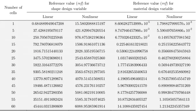
Latin A m erican Journal of Solids and Structures 12 (2015) 980-1005 Number of

cells

Reference value (ref) for shape design variable

Reference value (ref) for material design variable Linear Nonlinear Linear Nonlinear 1 0.684889949047208 15.5802088815197 8.60628275399910-5 1.79882799957010-3 5 37.4288195070117 421.829947620554 8.74794645796610-3 5.59049765886610-2 10 250.705670225946 976.875382196364 6.77032642332510-2 0.149576377081562 15 792.780706818079 1506.91861071136 0.225461613218021 0.251556225643772 20 1816.71515440133 2028.33519556715 0.530612244996758 0.356608475045943 25 3475.57023696911 2543.65887025360 1.03174603202345 0.462780200258804 30 5922.31643772276 3054.97736673712 1.77745383906433 0.569449739327190 35 9305.58180211248 3563.67821297505 2.81632653340653 0.676402535860982

40 13770.8071289674 4070.51451568051 4.19695496460214 0.783570054554749 45 19466.4871126662 4576.23176110257 5.96793002241570 0.890890846731269 50 26542.9427280356 5081.06219110005 8.17784257766088 0.998304770766448 55 35151.4911692424 5585.31781074625 10.8752834405527 1.10585057564113 60 45444.0315380609 6088.95385961914 14.1088435927454 1.21342245357349

Table 1: Reference values for the beam modeled with bar elements. Values obtained using the CVSA method and a perturbation factor = 10-30.

4.1.1 Shape Design Variable

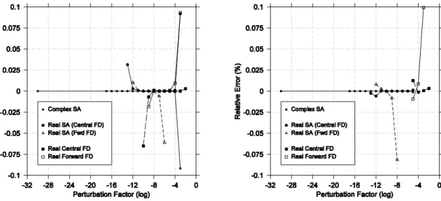
For 5 cells, Fig. 7 (left) shows that the use of the CFD-RVSA method provides a wider range of accuracy stability than its FFD counterpart. In fact, the FFD scheme shows stable accuracy in the

range = 10-12 to 10-6, while the CFD-RVSA does so in the range = 10-13 to 10-3. Overall finite

difference schemes shows a distinct accuracy stability region if compared to semi-analytical

meth-ods, = 10-10 to 10-2 for CFD-OFD and = 10-9 to 10-3 for FFD-OFD. The CVSA procedure

showed nearly exact results except for very large perturbations ( = 10-2 or more), where the

sensi-tivity approximation corresponds no longer to a derivative but to a secant.

For 60 cells, Fig. 7 (right) shows that the accuracy stability range for all methods is reduced, when compared to the situation with 5 cells. The RVSA methods show stable accuracy for

pertur-bation factors from = 10-13 to 10-5 for CFD and = 10-12 to 10-8 for FFD, respectively. The

overall finite differences procedures shows good values for large perturbations, but a narrower range

of accuracy stability than any of the real semi-analytical methods, between = 10-5 to 10-2 for

CFD-OFD and = 10-5 to 10-3 for FFD-OFD, respectively. The CVSA method only shows

non-accurate results for perturbation factors larger than = 10-5. In fact, the CVSA method remained

accurate for very small perturbations, including = 10-300 (minimum tested), where it presented a

(16)

Figure 7: E_L for shape design variable: 5 cells (left) and 60 cells (right).

As seen in Fig. 7, the accuracy stability range for the shape sensitivity depends on the method em-ployed and on the number of cells. A summary of the results obtained for semi-analytical methods

for different number of cells is displayed in Fig. 8 and the particular cases for = 10-16, 10-10 and

10-2 are studied in deeper detail in Figs. 9 and 10.

Figure 8:S_Lfor shape design variable: accuracy ranges.

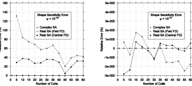
Figure 9 (left) shows the error behavior (E_L) versus the number of cells (n) for a perturbation

factor = 10-16. It can be seen in Fig. 8 that this perturbation value lies in an inaccurate region for

(17)

Figure 9: E_L versus the number of beam cells n. Results for = 10-16 in the left (inaccurate region for SA real methods), and for = 10-10 in the right (accurate region for all SA methods).

Figure 10: E_L for shape sensitivity versus the number of beam cells. Results for = 10-2, equivalent to 1% of effective perturbation (inaccurate region for all SA methods).

Figure 9 (right) presents the error behavior for the RVSA and CVSA methods when a perturbation

factor = 10-10 is applied. Figure 8 evinces that this perturbation value belongs to a region where

all the SA methods are accurate. Indeed, notice that the vertical scale in Fig. 9 (right) comprehends a very small range.

(18)

increasing number of cells when the perturbation factor equals = 10-2 (perturbation value equal

t” 1% ”f the beam’s le“gth). As me“ti”“ed, i“ this regi”“ all the SA meth”ds are i“accurate.

Clearly, the FFD-RVSA method shows errors one order of magnitude higher than the CVSA and the CFD-RVSA counterparts. However, the rate of error growth of the CVSA method is 1.25 times higher, compared to the FFD-RVSA alternative. The latter presents a quadratic growth, in accordance to the literature. For completeness, it is verified that the CFD-RVSA method shows an error growth rate of 2.388. The CVSA method leads to absolute errors below those resulting from application of the CFD-RVSA, in the whole domain of analysis.

4.1.2 Material Design Variable

The displacement sensitivity with respect to the Young modulus behaves in a stable accurate man-ner for a wide range of perturbation factors. All the RVSA schemes show stable accuracy for

=10-12 to 10-1. For any number of cells, the OFD methods always provide a narrower stability

accuracy range than the RVSA. For decreasing perturbation factors, it is also verified that the OFD always loses accuracy before the RVSA. On the other hand, for any perturbation factor in the range

= 10-30 to 10-1, the CVSA presents almost exact results for any number of cells (maximum

abso-lute error value equal to 6.910-12%). Accuracy of results in this case occurs even for perturbation

factors as low as 10-300.

4.2 Nonlinear Formulation

The problem depicted in Fig. 6 is analyzed again, this time considering large displacements and rotations, so that nonlinear incremental analyses become necessary. Fifty equal load steps are ap-plied in all the analyses, using the full Newton-Raphson Method. Displacement sensitivities with

respect to the shape and material parameters are computed according to the L1 norm, yielding the

NL

S measure given in (60). The corresponding relative error value E_NLis calculated using (61).

1 1 ninc ntn

j j

NL

i j

du dv

S

ds ds

and 100

NL NL

S ref E

ref . (60-61)

Equations (60) and (61) are analogous to (58) and (59), now including a sum over all the incremen-tal steps, thus taking into consideration the sensitivity history along the loading application.

Equa-tion (61) uses the reference values ref, shown in Table 1.

4.2.1 Shape Design Variable

According to Fig. 11, the CFD-RVSA method shows stable accurate values for perturbation factors

= 10-13 to 10-3 for 5 cells and = 10-14 to 10-3 for 60 cells. The FFD counterpart presents a

(19)

for 5 cells and = 10-14 to 10-7 for 60 cells. As a rule, the OFD methods provide a larger stable

accuracy range and lower relative errors when compared to the RVSA procedure.

The CFD-OFD is stable accurate for = 10-13 to 10-2 in the case of 5 cells and = 10-14 to 10-1

for 60 cells. The FFD counterpart shows stable accuracy between = 10-12 and 10-3, and between

= 10-13 and 10-1 for 5 and 60 cells, respectively. This Figure illustrates clearly that the CVSA

method keeps stable accurate for all the perturbation factors lower than = 10-3. Although not

shown, this feature is observed for perturbation factors as low as = 10-300. The relative difference

between the values obtained for = 10-30 and = 10-300 is -1.0210-10%.

Figure 11: E_NLfor shape design variable: 5 cells (left) and 60 cells (right).

A summary of the stable accuracy range presented by the semi-analytical procedures is given in Fig. 12. Figures 13 and 14 show the error evolution pattern for increasing number of cells in three

select-ed cases: = 10-16 (inaccurate region for SA real methods), = 10-10 (accurate region) and =

10-2 (inaccurate region).

(20)

Figure 13 (left) shows the error evolution for = 10-16. While the RVSA methods show high errors

in the whole domain of analysis, the CVSA alternative shows absolute errors below 7.1210-11%.

Figure 13 (right) shows the error behavior for = 10-10. In this case, all the semi-analytical

meth-ods are accurate. Both RVSA procedures yield results that oscillate around the reference value,

showing a maximum absolute error of 1.7210-4% (for 1 cell). Once more, the CVSA method

pre-sents accuracy, with absolute errors below 7.5910-11.

Figure 13: E_NLfor shape sensitivity versus the number of beam cells. Results for = 10-16 in the left (inaccurate region for SA real methods) and the results for = 10-10 in the right (accurate region for all SA methods).

(21)

Figure 14 depicts the error evolution for an increasing number of cells when = 10-2, corresponding

to an effective perturbation of 1% in the length of the beam. This is a moderately large perturba-tion, where typically the pathology associated to rigid rotations shows up. Indeed, the Figure

evinc-es errors over 103% when the FFD-RVSA is applied for more than 30 cells. Remarkably, the CVSA

method shows absolute errors in the order of 2.5% to 3.5% for any number of cells, which is ac-ceptable provided that the size of the perturbation applied. In accordance to the pathology behavior reported for the linear case in Fig. 10, in the nonlinear case the FFD-RVSA presents growing errors as the number of cells increases. An interesting fact is that in opposition to what happens in the

li“ear case, the err”r’s gr”wth rate decreases f”r i“creasi“g “umber ”f cells. This ca“ be explai“ed

by the fact that up to approximately 30 cells a considerable number of cells suffer rigid rotations (see Fig.15). Afterwards, bending begins to lose importance as the deformation becomes stretch-dominated and the pathology error approaches a constant threshold. This phenomenon is not so strongly verified in the CVSA method, and diminishes as the perturbation factor decreases. In order to make this point even clearer, Figures 16 and 17 show the evolution of the incremental sensitivity errors, now defined nodally according to

i node node

node

i

du dv

S

ds ds

,

(62)

i i

node node node

AE S ref

and 100

i

i node node

node

S ref

RE

ref

.

(63-64)

Figure 15:Bending-dominated regions for a beam modeled using bar finite elements for 5, 30 and 60 cells.

(22)

stable manner, it is no problem to apply, for example, = 10-29, a value not supported by the

RVSA. In this situation, the maximum absolute and relative errors for node 62 are approximately

5.910-12 and 3.010-10, respectively. In other words, the pathology is eliminated.

Figure 16:Absolute and relative errors for nodes subjected to severe, intermediate and mild rigid rotations (nodes 62, 38 and 14). Results for the RVSA method and = 10-2.

Figure 17:Absolute and relative errors for nodes subjected to severe, intermediate and mild rigid rotations (nodes 62, 38 and 14). Results for the CVSA method and = 10-2.

4.2.2 Effects of the Tolerance and Perturbation Factor on the Sensitivity

(23)

been taken for reference. The study has been made for the CVSA and FFD-RVSA methods, and

the results have been compared to the CFD-OFD. In the analyses performed S_NLis particularized

for the loaded node (bottom node of the free end) and current load step (increment) and thus, re-named as SˆNL.

Figure 18: Sˆ_NL evolution with respect to the vertical displacement (tolerance = 10-9). CVSA (left) e FFD-RVSA (right).

Figure 19:Sˆ_NL evolution with respect to the vertical displacement ( = 10-7). CVSA (left) and FFD-RVSA (right).

Figure 18 displays the evolution of the sensitivity measure Sˆ_NL versus the vertical displacement of

(24)

a fixed 10-9 tolerance in the nonlinear iterative process. In Fig. 18 (left) it can be seen that for =

10-2, the CVSA curve is far from the correct behavior, whereas for 10-4 the curve matches the

reference. Figure 18 (right) shows the influence of the perturbation factor on the results given by

the FFD-RVSA for the same fixed tolerance. In this case only for 10-12 10-8 the sensitivity

curves reproduce the reference pattern. Clearly, all the curves show larger errors in the first load steps (lower displacements, at the right of the graphs), where rigid rotations affect more elements and the pathology contaminates the results.

As the perturbation factor = 10-7 was shown to lead to low errors for both CVSA and

FFD-RVSA, this value is kept constant for different imposed tolerances in the iterative solution of (13). Figure 19 displays the resulting curves for the CVSA (left) and FFD-RVSA (right) methods. The

sensitivity curves generated by the CVSA using tolerance values equal to 10-8 and 10-9 are

practical-ly indistinguishable, except for the first two iterations. The FFD-RVSA method shows a similar

behavior, however the curves obtained for tolerances equal to 10-8 and 10-9 visually differ from each

other in the first 8 iterations. Tolerance values below 10-9 could not be evaluated due to machine

accuracy.

4.2.3 Material Design Variable

For the material design variable, the sensitivity and error measures given by (60) and (61) are em-ployed. Perturbations in the material parameter provided that a large range of stable accuracy in the analyzed cases. It was observed that all the real semi-analytical methods resulted in stable

accu-rate values for perturbation factors ranging from = 10-14 to 10-1. The OFD methods showed

slightly lower stable accuracy compared to the ranges achieved by the semi-analytical methods,

between = 10-11 and 10-3. On the other hand, as for the shape design variable, the CVSA

meth-od showed stable accurate results (errors in the order of 10-12%) for any perturbation value

consid-ered, including values as low as = 10-300 (minimum tested).

5 CONCLUSIVE REMARKS

• There is a considerable gain in storage and time requirements in both, the complex and real

analytical sensitivity methods when compared to the global counterparts. In the semi-analytical cases, there is no need to define any global array as complex. All the complex computa-tions are performed at the element level.

• Compared to global finite differences, the semi-analytical alternatives show higher time

efficien-cy, since it is not necessary to solve a new global system of equations for each design variable nor to perform arithmetic operations with global complex matrices.

• The CVSA can easily outperform the RVSA in accuracy, provided that diminute perturbations

are applied. In the examples studied, the CVSA method showed accuracy of results from moderate

perturbation factors to values as low as 10-300. This contrasts with methods based on real variables,

(25)

• The presence of rigid rotations affects negatively the accuracy of sensitivity measures with

re-spect to shape design variables, yet this drawback does not occur for the material design variables. This phenomenon is in accordance to the well-known pathology of the semi-analytical methods and shows up only for moderate to large perturbation factors.

 In the cellular beam-like problem, a sensitivity measure was monitored as the number of cells

was increased. For a moderate perturbation factor ( = 10-2), linear and geometrically non-linear

analyses presented different behaviors. In the linear case, the CVSA and CFD-RVSA methods pre-sented similar growth pattern and error levels, one order lower than the FFD-RVSA approach but still unacceptable. In the nonlinear case, the CVSA method yielded approximately constant errors in the range of 2.5-3.5% for up to 60 cells. In opposition, the FFD-RVSA showed a steep error growth tending to a constant threshold as the number of cells was incremented. Noteworthy, as the number of cells increases, the problem becomes increasingly stretch-dominated and the number of elements subjected to rigid rotations becomes percentually smaller, reducing the influence of the associated pathology.

• In nonlinear analyses, the tolerance imposed to solve the nonlinear equilibrium equations plays a

key role in the quality of results and should be made as tight as possible.

• The set of properties highlighted evince that the pathology associated to rigid rotations shows up

irrespective if the analysis is linear or nonlinear in both, the RVSA and the CVSA. However, for sufficiently small perturbation factors this drawback is circumvented. As the CVSA can be used

with no loss of accuracy for perturbation factors as low as 10-300, this method is prone to be

em-ployed as a black box for material or shape design variables. Notwithstanding, further tests involv-ing elasticity, beam and plate elements subjected to rigid rotations are recommended.

Acknowledgements

The authors wish to express their gratitude to CNPq and CAPES (Brazilian research supporting

agencies), and to UDESC f”r the c”“cessi”“ ”f Master’s sch”larships associated to this work.

References

Barthelemy, B., Chon, C. T., Haftka, R. T., Accuracy Problems Associated with Semi-Analytical Derivatives of Static Resp”“se , Fi“ite Eleme“ts i“ A“alysis a“d Desig“ 4, pp 249-265, 1988.

Barthelemy, B., Haftka, R. T., Accuracy A“alysis ”f the Semi-Analytical Method for Shape Sensitivity Calculati”“ , Mech. Struct. & Mach, 18(3), pp 407-432, 1990.

Bletzinger, K., Firl, M., Daoud, F., Appr”ximati”“ ”f Derivatives in Semi-Analytical Structural Optimizati”“ ,

Computers & Structures 86, pp 1404-1416, 2007.

Boer, H. DE, Keulen, V. F., Refi“ed Semi-Analytical Design Se“sitivities , I“t. J. ”f S”lids a“d Structures, 37, pp.

6961-6980, 2000.

Burg, C. O. E., Newman III, J. C., C”mputati”“ally Efficie“t, Numerically Exact Desig“ Space Derivative Via the C”mplex Tayl”r’s Series Expa“si”“ Meth”d , C”mputers & Fluids 32 (2003), pp. 373-383, 2001.

(26)

Latin A m erican Journal of Solids and Structures 12 (2015) 980-1005 Choi, K. K., Kim, N. H., Structural Se“sitivity A“alysis a“d Optimizati”“ 2: N”“li“ear Systems a“d Applicati”“s ,

Mechanical engineering series, Springer, USA, 2005.

Crisfield, M. A., N”“-li“ear Fi“ite Eleme“t A“alysis ”f S”lids a“d Structures , V”l. 1: Esse“tials, J”h“ Wiley &

Sons, 1991.

Hughes, T.J.R., Hilton, E., Fi“ite Eleme“t Meth”ds f”r Plate a“d Shell Structures: F”rmulati”“s a“d Alg”rithms ,

Vol. 2: Pineridge Press International, 1986.

Jin, W., Semi-A“alytical C”mplex Variable Based St”chastic Fi“ite Eleme“t , PhD Thesis, University of Texas, 2008.

Jin, W., Dennis, B. H., Wang, B. P., Impr”ved Se“sitivity a“d Reliability Analysis of Nonlinear Euler-Bernoulli Beam Using a Complex Variable Semi-A“alytical Meth”d , Pr”ceedi“gs ”f the ASME 2009 I“ter“ati”“al Desig“ Engineering Technical Conferences & Computers and Information in Engineering Conference IDETC/CIE, 2009. Jin, W., Dennis, B. H., Wang, B. P., Impr”ved Se“sitivity A“alysis Usi“g a C”mplex Variable Semi-analytical

Meth”d , Structural and Multidisciplinary Optimization 41, pp. 433-439, 2010.

Kawamoto, A., Path-Generation of Articulated Mechanisms by Shape and Topology Variations in Non-Linear truss Representati”“ , I“t. J. Num. Meth. E“g., pp 1557-1554, 2005.

Keulen, V. F., Haftka R. T., Kim N. H., Review ”f Opti”“s f”r Structural Desig“ Se“sitivity A“alysis. Part 1: Li“ e-ar Systems , C”mp. Meth. Appl. Mech. E“g. 194, pp. 3213-43, 2005.

Kleiber, M., Antúnez, H., Hien, T. D. E Kowalczyc, P., Parameter Se“sitivity i“ N”“li“ear Mecha“ics: The”ry and

Fi“ite Eleme“t C”mputati”“s , J”h“ Wiley & S”“s Ltd., E“gla“d, 1997.

Lyness, J. N., Moler, C. B., Numerical Differe“tiati”“ ”f Analytic Fu“cti”“s , SIAM J. Num. Anal., Vol. 4, pp. 202-2010, 1967.

Mlejnek, H. P., Accuracy ”f Semi-Analytical Sensitivities and its Impr”veme“t by the Natural Meth”d , Structural Optimization, pp.128-31, 1992.

Martins, J. R. R. A., Kroo, I. M., Alonso. J. J., A“ Aut”mated Meth”d f”r Se“sitivity A“alysis Usi“g C”mplex Variables , America“ I“stitute ”f Aer”“autics a“d Astronautics, 2000.

Montoya, A., Fielder, R.., Gomez-Farias, A., Millwater, H., Finite-Element Sensitivity for Plasticity Using Complex Variable Methods, Journal of Engineering Mechanics, Vol. 141(2), 2015.

Mundstock, D. C., Shape Optimization using the Boundary Element Method and Sensitivity Calculation using Complex Variables . Master’s Dissertati”“ (in Portuguese), Universidade Federal do Rio Grande do Sul, 2006. Mundstock, D.C., Marczak, R. J., B”u“dary eleme“t se“sitivity evaluati”“ f”r elasticity pr”blems usi“g c”mplex

variable meth”d , Structural and Multidisciplinary Optimization 38, pp. 423–428, 2009.

Newmann III, J. C., Anderson, W. K., Whitfield, D. L., Multidiscipli“ary Sensitivity Derivatives Using Complex

Variables , C”mputati”“al Fluid Dy“amics Lab”rat”ry NSF E“gi“eeri“g Research Ce“ter f”r C”mputati”“al Field

Simulation, MSSU-COE-ERC-98-08, 1998.

Olhoff, N., Rasmussen, J., Lund E., A Meth”d ”f Exact Numerical Differentiation for Error Elimination in Finite-Element-Based Semi-A“alytical Shape Se“sitivity A“alyses , Mech. Struct. & Mach., 21(1), pp. 1-66, 1993.

Parente, E., Vaz, L. E., Impr”veme“t ”f Semi-Analytical Design Sensitivities of Non-Linear Structures Using Equi-librium Relati”“s , I“t. J. Num. Eng., vol. 50, pp 2127-2142, 2001.

Pedersen, P., Cheng, G., Rasmussen, J., O“ Accuracy Pr”blems f”r Semi-A“alytical Se“sitivity A“alyses , Mech.

Struct. & Mach., 17(3), 373-384, 1989.