Lat. Am. j. solids struct. vol.12 número5

(1)

Abstract

For many practical applications in engineering, a complex struc-ture shows linear elastic behavior over almost all its extension, but exhibits confined plasticity contained in some small critical regions, e.g. stress concentrations in fillets and sharp internal corners. The behavior of C0- and Ck-GFEM is investigated in this class of problems.

The first goal of this study is to verify the actual formulation of the Ck-GFEM for two-dimensional elastoplasticity, as a modi-fication of the C0-GFEM formulation. The Ck-GFEM is based on a set of basis functions with Ck continuity over the domain. The approximation functions are constructed from a Ck continuous partition of unity, over which polynomial enrichment functions (or any special function) can be applied, in the same fashion as in the usual C0-GFEM. In this way, the finite element approxima-tions show continuous responses for both displacements and stresses across inter-element interfaces.

An investigation is performed to assess the behavior of higher-regularity partitions of unity against conventional C0 counter-parts. The irreversible response and hardening effects of the ma-terial is represented by the rate independent J2 plasticity theory

with linear isotropic hardening of material and von Mises yield criteria, being considered only monotonic loading and the kine-matics of small displacements and small deformations. The focus herein is to enlighten any possible advantage of smoothness in the presence of plastification phenomena, seeking for improve-ments in capturing the evolution of the process zone.

Keywords

Generalized Finite Element Method, smooth GFEM-based ap-proximations, two-dimensional elastoplasticity, convergence anal-ysis, process zone evolution.

Comparative Analysis of C

k

- and C

0 -GFEM Applied

to Two-dimensional Problems of Confined Plasticity

Andresa Freitas a, b Diego Amadeu F. Torres c Paulo de Tarso R. de Mendonça b Clovis Sperb de Barcellos b

a _{Universidade Federal da Fronteira Sul,}

Laranjeiras do Sul, PR, Brazil.

b _{Grupo de Análise e Projeto Mecânico}_–

GRANTE, Departamento de Engenharia Mecânica, Universidade Federal de Santa Catarina, Florianópolis, SC, Brazil.

c _{Departamento de Engenharia Mecânica.}

Universidade Tecnológica Federal do Paraná – UTFPR – Londrina, PR, Brazil.

*Author email:

[email protected], [email protected], [email protected], [email protected]

http://dx.doi.org/10.1590/1679-78251262

(2)

Latin American Journal of Solids and Structures 12 (2015) 861-882

1 INTRODUCTION

Certain local characteristics of boundary value problems, such as high gradient, singularities and discontinuities, can be successfully modeled with the use of the generalized finite element method (GFEM), since it allows using a priori knowledge about the solution of a problem in the form of enrichment functions.

Several studies have shown that GFEM has been used successfully in linear elastic fracture mechanics (Areias and Belytschko, 2005; Belytschko, 2001; Duarte et al., 2007; Laborde et al., 2005; Pereira et. al., 2010; Stazi et al., 2003; Tabarraei and Sukumar, 2008). However, a real structure is a very complex body with stress states whose values based on the linear elasticity may exceed the elastic limits. The works of Kim et al. (2009) and Kim et al. (2012) proposed a

GFEM with global-local enrichment functions (GFEMgl) to numerically generate proper

enrich-ment functions for three-dimensional problems with confined plasticity. According to Duarte and Kim (2008), the GFEMgl can be potentially more efficient than the standard GFEM or FEM. Kumar et al.(2014a) proposed an adaptive coupled finite element (FE) and element free Galerkin (EFG) approach used to simulate the nonlinear behavior of materials from two-dimensional sta-ble crack growth prosta-blems, where EFGM has been used only in a region near the crack, while FEM has been used away from the crack. In the work of Kumar et al.(2014b), XFEM has been extended to simulate stable crack growth by J_–R criterion, using finite strain plasticity under plane stress condition. They concluded that XFEM is an effective tool for modeling stable crack

growth in homogeneous and bi-materials as it does not require the conformal meshing.

The piecewise polynomial partition of unity (PoU) functions used in the conventional in-stance of the method may be not the most appropriate for some kinds of problems, as in case of

singular enrichments (Torres et al., 2014). In this context, the Ck-GFEM, which is quite similar

to C0-GFEM, presents the high regularity of the approximation as an attractive feature. This smooth version of GFEM is a mesh-based discretization methodology which brings together high-er regularity, flat-top prophigh-erty, globally defined coordinates, compact support and no restriction regarding the shape of elements and/or clouds.

The importance of Ck-GFEM comes from the fact that it is more robust than other kinds of

higher regularity mesh-based approximations. Some C1 approximants applied to problems that require such regularity, as Hermitian functions commonly used in thin plate bending problems, for instance, are very restrictive and do not favor a systematic procedure for building such func-tions for general element shapes or to allow p-refinement. Some approaches that exploit some

benefits of Ck-GFEM approximations in plate bending problems were presented in Barcellos et al.

(2009), Mendonça et al. (2011) and Mendonça et al. (2013).

(3)

The irreversible response and hardening effects of the material is represented by rate inde-pendent J2 plasticity theory with linear isotropic hardening of material and von Mises yield

crite-ria, being considered only monotonic loading and the kinematics of small displacements and small deformations.

The paper is structured as follows. Section 2 briefly describes the C0-GFEM, which is used as

a starting point for the Ck-GFEM formulation developed in section 3. Section 4 presents the key

elements on the elastoplasticity model considered herein, section 5 describes the test problems and presents the numerical results. Section 6 develops several concluding remarks about the findings.

2 GENERALIZED FINITE ELEMENT METHOD (C0-GFEM)

The GFEM is a combination of the standard finite element method (FEM) with concepts and techniques typical of meshless methods. This method presents an aspect of nodal enrichment that, in many situations, reduces or avoids the need of localized mesh refinement, making it very attractive for several analyzes.

The GFEM relies on a mesh that is used to define a partition of unit (PoU) and a domain for the numerical integration over which the enrichment of the PoU functions is performed. The set of PoU functions is employed to ensure the inter-elementar continuity, providing conformity of approximations that are improved by nodal enrichment strategy.

The enrichment functions are linked to individual clouds (patches) of elements around an ar-bitrary node in order to improve the quality of approximation in that neighborhood. Thus, one has the possibility to enrich the approximation only in a region of the problem domain, due to the compact support of PoU, without mesh refinement (Duarte et al., 2000), (Barros et al., 2004). Moreover, the essential boundary conditions can be imposed exactly as in the standard FEM (Strouboulis et al., 2001).

To build the GFEM approximation functions it is considered, for example, a conventional mesh of finite elements defined by N nodes with Cartesian coordinates in the domain _Ω. In plane problems, usually the elements are three node triangles or four nodes quadrilaterals (and

analogously in three-dimensional meshes). If the enrichment is performed with relation to node ,

a generic cloud is defined as the union of all finite elements adjacent to this node. The set

of the shape functions belonging to each element associated with the node , compose the

func-tion on the support of the cloud . The set of functions associated to all nodes on the domain form a partition of unity (PoU). The enrichment functions related to the node , are denoted by (with ) and represent a set of q + 1 linearly

independent functions.

Enrichment functions can be chosen as polynomial functions, harmonic, anisotropic or even functions that are part of the solution of the boundary value problem (Babuska et al., 2002; Stroubouliset al., 2000; Melenk and Babuska, 1996). The local approximation subspaces can be

denoted as which may also be enriched according to an adaptive method. In

(4)

stands for the space of polynomials of degree less than or equal to p. For example, for p = 2 (quadratic basis), the set of enrichment functions is

where are nodal coordinates of an arbitrary node j and and are the cloud characteristic

dimensions around the node in the directions x and y, respectively.

Thus, the GFEM approximation functions associated to the node result from the

ex-trinsic enrichment of PoU, i.e., multiplying the PoU function with support on the cloud by

components of :

(no sum on j) (1)

This implies an increasing in the number of unknowns per node in relation with those associated with the PoU.

The resulting approximation function contains features of both functions, that is, the compact support of PoU and the approximation feature of the enrichment functions . The structure of GFEM offers more freedom in the choice of approximation functions compared to the standard FEM. The extrinsic way of to incorporate the algebraic refinements enables to vary the enrichment along the domain without compromising the conformity, which is ensured by the compact support of the PoU.

The generalized global approximation for the displacement on , denoted as

, can be written as a linear combination of approximation functions associated with

each node. The component , for example, can be written as:

(2)

where is a vector containing the full set of approximation functions and is a vector

contain-ing the nodal parameters and associated, respectively, with the PoU functions and the

enriched functions . The continuity of the function on the whole domain is guaranteed

by the characteristics of the PoU used.

2.1 Model Problem for Two-dimensional Elasticity

Let a boundary value problem (BVP) defined in a linear elastic domain , where the strong

form of equilibrium equations is given by

(3)

where is the vector containing the stress tensor components, is the vector of body

(5)

Neumann conditions are defined, respectively; and are prescribed displacements and tractions,

respectively, and is the unit outward normal to . The operator have their definitions

adapted to the vector notation considered for (see Zienkiewicz and Taylor (2005) for example)

and the superscript T indicates transpose. The Cauchy stress is related to the displacement

by the linear elastic relation , where is the vector containing the strain tensor

components end is the constitutive matrix of the material, which is positive definite.

The variational form of this problem can be stated as: Find such that:

(4)

where and are Hilbert spaces of degree order 1 (standard Sobolev space of square integrable functions whose first derivatives are also square integrable in the Lebesgue sense) de-fined on the domain Ω. The variational operators are defined as:

(5)

(6)

where is the vector of displacements, is the test function vector, is the

vector containing the strain tensor components, and is the thickness of the elastic body (in the

z reference direction) considered here as constant.

The Galerkin approximation in Eq.(4), similarly to FEM, results in:

Find such that: , (7)

whit and are being subspaces of finite dimension, wherein the first space is generated by

the approximation functions and the second one is of test functions; is composed according to

Eq.(2) and the component , for example, of the is given by:

(8)

where is a vector of nodal parameters similar to vector .

The only difficulty in the GFEM implementation is that the enriched basis can be linearly dependent, so that the system of equations resulting from Eq. (7) is positive semi-definite. The linear dependence occurs when the PoU and enrichments are both polynomial functions. This

problem can be avoided by careful choice of functions (Oden et al., 1998), constraints in PoU

(6)

3 ARBITRARY CONTINUOUS FUNCTIONS (CK-GFEM)

Ck-GFEM is quite similar to C0-GFEM, except that it builds an arbitrarily smooth PoU over finite element meshes (Duarte et al., 2006). Although this is not a meshless method, it preserves several attractive features of meshless approximations, such as the high regularity of

approxima-tion and partiapproxima-tion of unit property. The Ck-GFEM is also important because it can be efficiently

applied to higher-order problems, as the plate problems of Kirchhoff and Reddy, which require solutions of continuity at least C1.

The PoU functions can also be built as C functions in case of clouds with convex support

and considering exponential edge functions (the original Edwards (1996) procedure). In clouds with non-convex support they can be up to k-times continuously differentiable at the concave nodes, with k arbitrarily large, and infinitely differentiable in the rest of the cloud.

The technique used for the construction of PoU functions in the problems under analysis (Section 5), is described below for clouds with convex support and exponential edge functions (Edwards method).

Let us consider a conventional triangular finite element mesh defined by N nodes with coor-dinates in the domain Ω, and a set of weighting functions , with j = 1, ...,

N. Each one is associated to a cloud as its compact support. _{Using Shepard’s formula}

(Shep-ard, 1968), each PoU function is obtained by:

. (9)

Herein, triangle elements are considered aiming to employ them as integration cells directly, noting that the procedure is quite general for different element shapes or cloud configurations.

It can be seen that the set is such that , and

and any compact subset of _Ω intercepts only a finite number of supports. Therefore,

is a partition of unity and its regularity depends only on the regularity of the weighting functions constructed to ensure the required continuity.

The weighting functions with convex support can be built from the product of the cloud edge

functions associated with the cloud and defined in terms of parametric coordinates

normal to each edge n of de cloud (Barcellos et al., 2009 and Duarte et al., 2006

)

as follows:

, (10)

where is the number of edge functions to the cloud .

Thus, the Shepard equation is used to define a partition of unity from weighting functions continuously differentiable, using exponential edge functions. According to Edwards (1996), a cloud edge function is a strictly positive function inside the cloud which vanishes, together with

all its derivatives, towards an edge, rendering a weighting function.

(7)

dis-Latin American Journal of Solids and Structures 12 (2015) 861-882

tance from node j to the edge n. For these two conditions, was used the following function edge (Barcellos et al., 2009):

, (14)

where and is the distance between the position and the

edge n, is the edge midpoint, and the normal vector to the edge directed into the cloud.

and are positive arbitrary constants. However, numerical experiments have shown that the most appropriate values are and , as suggested by Duarte et al. (2006) and Torres (2012). Therefore, at cloud node the function has the value

(15)

which is the same for every edge n of the cloud and imposing the constraint ,

one gets .

It should be remarked that different choices of PoU functions are possible (it depends on the choice of the edge functions (Barcellos et al., 2009)), leading to different kinds of approximation functions.

However, besides exponential functions, many functions meet the requirements of having de-rivatives null on the edge. For example, in Barcellos et al. (2009) polynomial edge functions were subjected to numerical investigations. In this case of polynomial cloud edge functions, differently, the continuity is limited independently of the cloud geometry.

Herein, exponential edge functions are used, following the procedure described in Barcellos et al. (2009) which guarantee C(_) approximation for meshes with only convex clouds. On the contrary, in the case of non-convex clouds, it is necessary to replace the edge functions of a pair of non-convex edges with a single new edge function obtained through a boolean product (Rvachev and Sheiko, 1995) before performing the weighting functions computation, as proposed by Duarte et al. (2006). Therefore, the resulting PoU is at least k-times continuously differentia-ble, and the resulting approximation functions of the product of Shepard PoU with the enrich-ment functions will have the same continuity, since the enrichenrich-ments are at least also Ck.

4 TWO-DIMENSIONAL PLASTICITY

This section presents the equations that govern the classical plasticity in the two-dimensional context, which can be found in Chen (1988), Simo and Hughes (1998) and Souza Neto et al. (2008).

The formulation adopted is based on the classical rate independent J2 flow theory for small

(8)

Initially the isotropic hardening will be used, however, kinematic hardening and cohesion models can easily be introduced to the algorithm. The plastic flow is regarded as an irreversible process and is characterized in terms of the history of the following variables: strain tensor , plastic strain tensor and isotropic hardening internal variable , related to the evolution of plastic deformation.

Considering the additive decomposition of the total strain tensor , the isotropic linear elastic constitutive tensor , the deviatoric stress tensor s and the yield stress , the equa-tions that govern the model are:

1) elastic stress-strain relationship: ;

2) von Mises yield criterion: , where e is the modulus

plas-tic of isotropic linear hardening;

3) flow rule: , where ; 4) hardening law: ;

5) accumulated plastic deformation rate: ;

6) Kuhn-Tucker complementary conditions: , , ;

7) consistency condition: (if , where is the yield function rate.

The parameter is a non-negative function, called consistency parameter, which repre-sents the plastic flow rate satisfies the Kuhn-Tucker and consistency conditions.

5 NUMERICAL RESULTS

In this section, two numerical experiments are conducted. The goal is to compare the Ck-GFEM

and C0-GFEM performances for two-dimensional elastoplastic problems. The elastoplasticity

al-gorithm was introduced in a code developed for linear elastic fracture mechanics (Torres, 2012). The numerical experiments were conducted considering regular and uniform triangular mesh-es, with simplex elements, for which only convex clouds occur, in such a way that the functions

are C continuous for the smooth version of GFEM.

The algebraic refinement consists of uniformly applied polynomial enrichment functions of

degrees p = 1 to 4. The numerical integration on the elements was performed by the Wandzura’s

symmetric quadrature in triangles (Wandzura and Xiao, 2003) with 175 points. The same

quad-rature was used for the Ck-GFEM and C0-GFEM independently of the p-enrichment applied. It is

worth noting that this amount of integration points is used here only for sake of evaluation, to reduce the errors due to integration from discretization errors to negligible levels. For integrations in the Neumann boundary was used the Gauss-Legendre quadrature with 25 points, for each ele-ment edge.

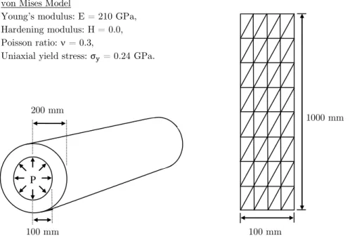
5.1 Internally Pressurized Cylinder

(9)

axisymmet-Latin American Journal of Solids and Structures 12 (2015) 861-882

ric elements. The maximum pressure, P, used to this problem was 0.18 GPa. Nine uniform pseu-do time steps were used for incremental analysis.

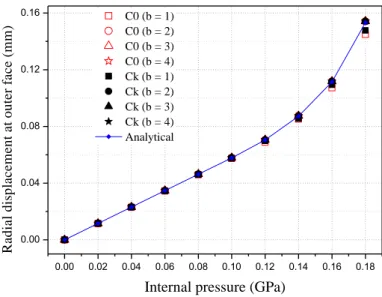
Figure 2 shows the radial displacement at outer surface of the cylinder versus applied

pres-sure computed by the C0-GFEM and Ck-GFEM for b = 1, 2, 3 and 4, that represents the

poly-nomial degree of reproducibility of the proposed GFEM approximation subspace. Figure 3 and Table 1 show the norm of the relative error of the radial displacement at outer face versus de-grees of freedom obtained via C0-GFEM and Ck-GFEM for the maximum pressure level (P =

0.18 GPa). On notice that b = p +1 to C0 PoU and b = p to Ck PoU, where p is the degree of

the polynomial enrichment, as identified in Mendonça et al. (2011). The relative error of the radi-al displacement is computed by , where and are the exact (Hill, 1950)

and approximated displacements, respectively.

Figure 1:Internally pressurized cylinder. Material properties and finite element mesh adopted.

It can be observed that the C0-GFEM and Ck-GFEM results are close to the analytical value and

exhibit similar errors for the same values of b. As expected, the worst values of the approxima-tions of displacement occur for b = 1. According to Figure 2, the approximation of the displace-ment for b =1 worsens at pressures above the yielding pressure onset, whose analytical value is

0.103 GPa (Souza Neto et al., 2008). This suggests that for this problem (choice of mesh, PoU,

enrichment function) both methods do not approach well the plastic solution when b = 1.

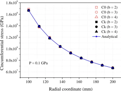
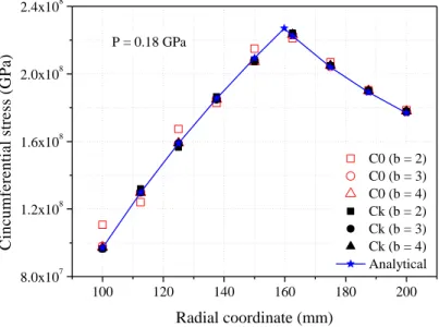
The circumferential stress obtained at integration points for P = 0.1 GPa (elastic solution) and P = 0.18 GPa (elastoplastic solution) are plotted for b = 2, 3 and 4 in figures 4 and 5

respec-tively, together with Hill’s solution. The C0-GFEM and Ck-GFEM results are very close to the analytical solution. The worst results occur for C0-GFEM when b = 2, where p = 1. For the

von Mises Model

Young’s modulus: E = 210 GPa,

Hardening modulus: H = 0.0, Poisson ratio: _ = 0.3,

Uniaxial yield stress: = 0.24 GPa.

100 mm 200 mm

P

100 mm

(10)

complete loading in case of P = 0.18 GPa, the plastic front reaches approximately 159.79 mm (analytic value of the radius of plastic zone). The approximate position of the elastoplastic transi-tion zone can be visualized by the positransi-tion of sign change in the slope of the curves in Figure 5.

Figure 2: Radial displacement versus increasing pressure for the problem of Figure 1.

Figure 3: Norm of relative error for the radial displacement at outer face versus degrees of freedom for the problem of Figure 1 for P = 0.18 GPa.

0.00 0.02 0.04 0.06 0.08 0.10 0.12 0.14 0.16 0.18 0.00

0.04 0.08 0.12 0.16

R

a

d

ia

l

d

is

p

la

c

e

m

e

n

t

a

t

o

u

te

r

fa

c

e

(

m

)

Internal pressure (GPa)

C0 (b = 1) C0 (b = 2) C0 (b = 3) C0 (b = 4) Ck (b = 1) Ck (b = 2) Ck (b = 3) Ck (b = 4) Analytical

0 180 360 540 720 900 1080 1260 1440 0.00

0.01 0.02 0.03 0.04 0.05 0.06

|er(

u

)|

DOF

(11)

Latin American Journal of Solids and Structures 12 (2015) 861-882 5.2 L-shaped Domain

The L-shaped domain is a classical problem of the elasticity theory for which an analytic solution is known (Szabo and Babuska, 2011). An elastoplastic version of this problem is considered here aiming (a) to verify the implementations for a general two-dimensional loading condition, (b) to investigate the effects of smooth discretization in the approximate stress fields, and (c) to com-pare the evolution of a process zone at the reentrant vertex neighborhood for the two kinds of regularity considered.

DOF

C0-GFEM Ck-GFEM

b |er(u)| b |er(u)|

90 1 0.05492 (5.49%)

270 2 0.005871 (0.58%) 1 0.03653 (3.65%) 540 3 0.006327 (0.63%) 2 0.005545 (0.55%) 900 4 0.006915 (0.69%) 3 0.006337 (0.63%)

1350 4 0.006915 (0.69%)

Table 1: Relative error values for the radial displacement considering different degrees b for the problem of Figure 1 for P = 0.18 GPa.

Figure 4: Circumferential stress versus radial coordinate to P = 0.1 GPa (elastic solution) for the problem of Figure 1.

The dimensions, material parameters, loading and mesh (Mesh 1) used in this example are shown in Figure 6. The analysis is carried out assuming plane strain conditions. The domain of the prob-lem is discretized by 96 eprob-lements. Ten uniform pseudo time steps were used for incremental

anal-ysis. The numerical results are compared with a overkill solution from ANSYS® (Reference 1) for

100 120 140 160 180 200

6.0x107 8.0x107 1.0x108 1.2x108 1.4x108 1.6x108 1.8x108

C

in

c

u

m

fe

re

n

ti

a

l

st

re

ss

(

G

P

a

)

Radial coordinate (mm)

C0 (b = 2) C0 (b = 3) C0 (b = 4) Ck (b = 2) Ck (b = 3) Ck (b = 4) Analytical

(12)

which was used a very refined regular and uniform triangular (3 nodes) mesh with 60 000

ele-ments and 60 799 degrees of freedom. It should be remarked that for the L-shaped domain prob-lem, considering elastic material, an infinity stress value occurs at the reentrant corner for the minimum amount of applied external force. This means that in the physical problem, in case of elastoplastic material, the yield criteriais reached once any external force is applied. Of course, for discretized problems, this fact is generally not true.

Figure 5: Circumferential stress versus radial coordinate to P = 0.18 GPa (elastoplastic solution) for the problem of Figure 1.

Figure 6: L-shaped domain. Material properties and finite element mesh (Mesh 1). The blue region is defined to allow the computation of a local deformation energy.

100 120 140 160 180 200

8.0x107 1.2x108 1.6x108 2.0x108 2.4x108

P = 0.18 GPa

C

in

c

u

m

fe

re

n

ti

a

l

st

re

ss

(

G

P

a

)

Radial coordinate (mm)

C0 (b = 2) C0 (b = 3) C0 (b = 4) Ck (b = 2) Ck (b = 3) Ck (b = 4) Analytical

von Mises Model

Young’s modulus: E = 210 GPa, Domain dimension: a = 100 mm,

Hardening modulus: H = 10.5GPa, Thickness constant and unitary: = 1 mm, Poisson ratio: _ = 0.3, Surface forces F1 = 500 N,

(13)

The strain energy, defined as , is used as a global convergence

measure to verify the numerical implementation. Another mesh with 384 triangular elements (Mesh 2, see Figure 7), was used in this verification, where the blue region is defined to allow the computation of a local deformation energy.

Figure 7: Finite element mesh (Mesh 2).

Tables 2 and 3 show values of the strain energy obtained by the Ck-GFEM and C0-GFEM for

different values of b, and to Meshes 1 and 2. Table 2 shows the strain energy calculated through-out the domain and Table 3 shows the correspondent value for the blue region of the meshes shown in figures 6 and 7, which approximately contains the plastic zone. One can see that the

results obtained by the C0-GFEM (Mesh 2) is greater than Reference 1 values, for some degrees

b, which would indicate the reference solution is still inappropriate. For this reason the numerical

results are also compared with the overkill solution from ANSYS® which is similar to the first

one but with triangles of 6 nodes (Reference 2), totaling 241 599 degrees of freedom. It is easy to see the present GFEM solutions converge to this new reference solution (Reference 2) as the de-gree b increases. Although the results for C0 are closer to the reference value as the degree b in-creases, in both situations the results of Ck for b = 1 are better, indicating some higher ability of the smooth functions of to capture the plastification for lower degree approximations. Latter, the evolution of the plastic zone will be investigated trying to confirm this hypothesis.

Table 4 lists the number of iterations in the Newton-Raphson scheme required in each

load-ing step obtained by C0-GFEM and Ck-GFEM (Mesh 1), for b = 1, 2, 3 and 4. The table

indi-cates that the total numbers of iterations required for both approaches are almost the same. The loading level for which the plastic flow threshold is reached has number of iterations different from 1. It is possible to note (see Table 4) that for b = 2 and 3 the plastic flow starts at the

same loading level for both conventional C0-GFEM and smooth GFEM. However, for the lower

approximation degree (b = 1) the Ck-GFEM is capable of detecting hardening two load steps

before the conventional counterpart, thanks to the derivatives of the Ck-PoU, which are not

con-stant inside the elements. Thus, it can be seen that in case of lower degree approximations, even

for coarse meshes, the Ck-GFEM captures the plastic flow in a lower loading level if compared to

the C0-GFEM. In case of elastic materials, it is known the appropriate patterns of mesh

refine-D

(14)

ments which should be applied close to these points. However, for more general kinds of geomet-ric details, or in case of elastoplastic materials, the definition of an optimal mesh-refinement could be a difficult task. From these facts, it seems to be interesting to use higher regularity functions around reentrances, or other geometrical details.

(/10-4) Reference

b 1 2 3 4 -

Mesh 1 C

0_-GFEM _1.9569175 _2.7690565 _2.9777273 _3.0790066

Reference 1 3.0868053x104 Ck-GFEM 2.0477177 2.6521702 2.8549167 2.9365689

Mesh 2 C

0_-GFEM _2.3747066 _2.9808580 _3.0891456 _3.1421370 _{Reference 2}

Ck-GFEM 2.4450268 2.9151004 3.0312286 3.0729354 3.1723654x104

Table 2: Values of total strain energy for b = 1, 2, 3 and 4.

(/10-4) – Close to the reentrance Reference

b 1 2 3 4 -

Mesh 1 C0-GFEM 0.555022 1.005259 1.105433 1.148006 Reference 1 1.1576717x104 Ck-GFEM 0.673580 0.985863 1.076643 1.106115

Mesh 2 C0-GFEM 0.819017 1.111261 1.165939 1.185627 Reference 2 1.1920987x104 Ck-GFEM 0.892644 1.097050 1.148191 1.160055

Table 3: Strain energy content within the sub-domain close the reentrance for b = 1, 2, 3 and 4.

Number of iterations

b 1 2 3 4

Reference 2 Load

step C

0_{-GFEM C}k_{-GFEM C}0_{-GFEM C}k_{-GFEM C}0_{-GFEM C}k_{-GFEM C}0_{-GFEM C}k_-GFEM

1 1 1 1 1 1 1 1 1 3

2 1 1 1 1 1 1 3 1 4

3 1 1 2 2 3 3 4 3 3

4 1 3 4 4 3 4 4 4 3

5 1 3 4 4 4 5 4 4 3

6 4 4 4 5 5 5 5 4 3

7 3 4 4 4 5 4 5 4 3

8 2 4 5 4 5 4 4 4 3

9 3 4 4 5 5 4 6 8 3

10 4 4 5 5 5 5 6 8 4

Total 21 29 34 35 37 36 42 41 32

(15)

The respective numbers of degrees of freedom used in C0-GFEM and Ck-GFEM analyses for

dif-ferent values of b are shown in Table 5.

Table 6 shows values of displacements in the y direction at points B and C for the Mesh 1

(see Figure 6) and the relative errors obtained by the Ck-GFEM and C0-GFEM for different

de-grees b.It can be notedthat the convergence of both forms of GFEM when the degree b increases

is clear, and it is seen that only for b = 1 the values obtained by Ck-GFEM exhibits smaller

er-rors than those obtained by C0-GFEM. These results suggest that the approximation subspace generated by the Ck-GFEM is "less flexible" than that for the C0-GFEM since, for the same

number of degrees of freedom and higher degrees of b, the error obtained by Ck-GFEM increases.

This observation agrees with the understanding that Ck _ C0.

C0-GFEM Ck-GFEM C0-GFEM Ck-GFEM C0-GFEM Ck-GFEM C0-GFEM Ck-GFEM

b 1 2 3 4

DOF (Mesh 1) 130 390 390 780 780 1300 1300 1950

DOF (Mesh 2) 450 1350 1350 2700 2700 4500 4500 6750

Table 5: Quantities of degrees of freedom for b =1, 2, 3 and 4 to Meshes 1 and 2.

b uy (|er(uy)|)

point B point C

C0-GFEM 1 2 3 4

0.3568 (34.80 %) 0.4900 (10.46 %) 0.5251 (0.405 %) 0.5433 (0.073 %)

0.6015 (42.56 %) 0.9363 (10.59 %) 1.0090 (3.657 %) 1.0420 (0.506 %)

Ck-GFEM 1 2 3 4

0.3721 (32.01 %) 0.4719 (13.77 %) 0.5058 (7.582 %) 0.5197 (5.042 %)

0.6440 (38.50 %) 0.8997 (14.09 %) 0.9683 (7.543 %) 0.9954 (4.955 %)

Reference 2 - 0.5473 1.0473

Table 6: Values of displacements in the y direction at points B and C (Figure 6) and relative error (in parentheses).

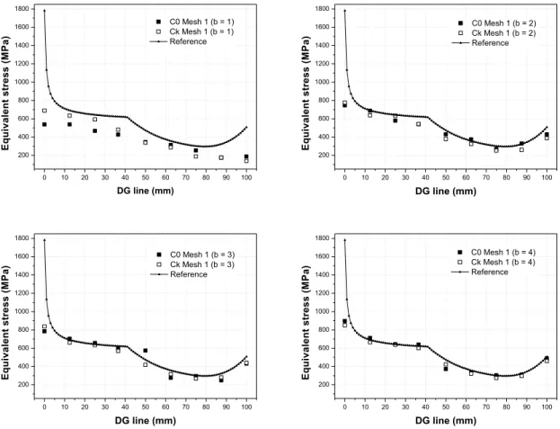
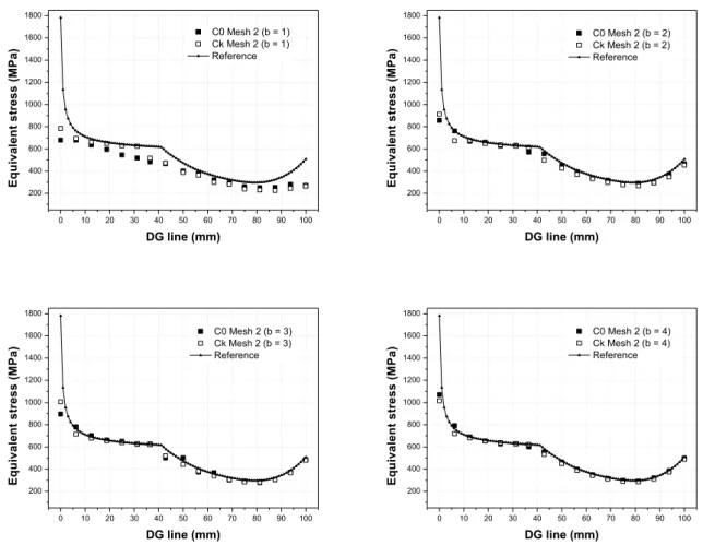
Figure 8 and 9 shows pointwise values of equivalent stress over the line DG in the meshes 1 and

2, respectively (see Figure 6 and 7), obtained by the Ck-GFEM and C0-GFEM, for b = 1, 2, 3

and 4. Whereas that in the C0-GFEM was performed an average of nodal values, clearly Ck

-GFEM and C0-GFEM are not confronted with the same rigor. In general, the results obtained by

Ck-GFEM are closest to the reference solution (Reference 2) when compared with the results

ob-tained by C0-GFEM. For b = 3 and 4, the right side of the curves for Ck-GFEM is already good

(16)

The figure shows that better results could be achieved with a refined mesh. For example, the use of a graded mesh would capture singularity at a lower loading level, and therefore the plastic flow. Additionally, an algebraic refinement consisting of non-uniformly applied polynomial en-richment functions, such as considering higher b degree towards the reentrance, would also be used, or even another kind of enrichment function. However, the costs are reduced using a coarse

mesh and smaller values of b, and in this case the Ck-GFEM presents better results compared to

C0-GFEM.

Figure 8: Values of equivalent stress over the line DG to Mesh 1 (see Figure 6).

It can be noted that for Mesh 2 and b = 4 the difference in equivalent stress at the extreme left point of the line DG is still very large, as the exact solution is singular, due to the linear harden-ing, and only polynomial basis functions were used, without any special refinement toward the reentrant corner. Then, for verification purposes a geometric mesh (see definition in Szabo and Babuska, 2011) with 72 triangular elements (Mesh 3, see Figure 10), was used in this verifica-tion. Figure 11 shows pointwise values of equivalent stress over the line DG in Mesh 3, obtained

by the Ck-GFEM and C0-GFEM, for b = 1, 2, 3 and 4. In general, the results obtained by Ck

-GFEM and C0-GFEM are similar, and for b = 3 and 4, the curves agree very well, even at the

0 10 20 30 40 50 60 70 80 90 100

200 400 600 800 1000 1200 1400 1600 1800 E q u iv a le n t s tr e s s ( M P a )

DG line (mm)

C0 Mesh 1 (b = 1) Ck Mesh 1 (b = 1) Reference

0 10 20 30 40 50 60 70 80 90 100

DG line (mm)

0 10 20 30 40 50 60 70 80 90 100

DG line (mm)

0 10 20 30 40 50 60 70 80 90 100

DG line (mm)

(17)

extreme left point. Note that although the exact solution is infinite at point D, the reference solu-tion is finite at this point, since it is numerically calculated and uses a base that belongs to a space of regular functions. Figure 12 shows the relative error of equivalent stress at D point, with respect to the reference solution, versus degrees of freedom obtained via C0-GFEM and Ck -GFEM. It is observed that the convergence in geometric mesh is much faster than in other ones, as expected.

Some influence of smoothness can also be seen from the geometric aspect of the process zones for different degrees b at the end of loading. Figure 13 shows distributions of integration points where the yield condition was reached for the complete loading. This figure compares the Ck -GFEM and C0-GFEM performances considering the high gradient of deformation field that oc-curs in the plastic zone. The results suggest the ability of the approximation functions with arbi-trary inter-element continuity to represent the plastic zone more properly than the C0, mainly for lower degree approximations, as early mentioned (see reference solution in the Figure 14).

0 10 20 30 40 50 60 70 80 90 100

DG line (mm)

0 10 20 30 40 50 60 70 80 90 100

DG line (mm)

0 10 20 30 40 50 60 70 80 90 100

DG line (mm)

0 10 20 30 40 50 60 70 80 90 100

DG line (mm)

(18)

Figure 10: Finite element mesh (Mesh 3).

0 10 20 30 40 50 60 70 80 90 100

DG line (mm)

0 10 20 30 40 50 60 70 80 90 100

DG line (mm)

0 10 20 30 40 50 60 70 80 90 100

DG line (mm)

0 10 20 30 40 50 60 70 80 90 100

DG line (mm)

(19)

Figure 12: Relative error of equivalent stress versus degrees of freedom for the problem of Figure 6.

C0-G FEM

b_{= 1} b_{= 2} b_{= 3} b_{= 4}

Ck-G FEM

b_{= 1} b_{= 2} b_{= 3} b_{= 4}

Figure 13: Locus of integration points for which the yield condition was reached, for the problem of Figure 6.

100 1000 10 R e la ti v e e rr o r o f e q u iv a le n c e s tr e s s ( % ) DOF

C0 Mesh 1 C0 Mesh 2 C0 Mesh 3 Ck Mesh 1 Ck Mesh 2 Ck Mesh 3

-100 -50 0 50 100 150 -150 -100 -50 0 50 100 150

(20)

6 CONCLUSIONS

The aim of this study was to verify the GFEM implementation for two-dimensional elastoplasticity, and after that, compare through numerical experiments the Ck-GFEM and C0

-GFEM performances in problems with confined plasticity based on J2 plasticity theory. For the

two problems analyzed such comparison was performed using local and global convergence measures.

The results presented for the pressurized cylinder problem show that the quality of the stress

is almost the same for both C0-GFEM and Ck-GFEM, for the same degree of the approximation

b. That is expected considering that this problem is essentially one-dimensional.

On the other hand, the results presented for the L-Shaped problem suggest that the Ck -GFEM furnishes better approximations for the plastic region boundary and the equivalent stress

values, mainly in the neighborhood of the reentrance, when compared with C0-GFEM.

Further-more, for b = 1 the Ck-GFEM presents better results when compared to those obtained by C0

-GFEM. This observation comes from the fact that the Ck PoU functions have non-constant

de-rivatives inside the elements, differently from C0 tent functions, which favor capturing much

lo-calized features even using coarse meshes. Then, as can be seen in Table 4 (for b = 1), since the

smooth PoU functions enable the detection of hardening for smaller load if compared to the C0

continuous counterpart, it can be argued that the Ck PoU functions around critical points are more appropriate for determination of a load level with cause plastic flow in the structure.

Finally, these are the first exploratory results towards a larger work which aims to use the Ck-GFEM for composing local problem of the Global-Local GFEM (GFEMgl). One of the next

steps of this research is to keep the process of checking of the L-shaped problem, where

investiga-tions will be conducted to reduce costs by applying smooth PoU funcinvestiga-tions only in the region of the recess, using coarse mesh and small b.

(21)

Acknowledgments

The authors gratefully acknowledge the financial support provided by the Brazilian government agency CNPq (Conselho Nacional de Desenvolvimento Científico e Tecnológico) for this research under the grants 163.461/2012-0 (D. A. F. Torres), 304.698/2013-0 (C. S. de Barcellos) and 304.702/2013-7 (P. T. R. Mendonça).

References

ANSYS® (2010) User's manual. ANSYS Inc, USA.

Areias, P. M. A., Belytschko, T., (2005). Analysis of three-dimensional crack initiation and propagation using the extended finite element method. International Journal for Numerical Methods in Engineering, v. 63, pp. 760-788. Babuska, I., Banerjee, U.and Osborn, J.E., (2002). On principles for a selection of shape functions Generalized Finite Element Method. Computer Methods in Applied Mechanics and Engineering, v. 191, pp. 5595-5629. Babuska, I., Banerjee, U., Osborn, J.E., (2004). Generalized finite element methods - main ideas, results and perspective. International Journal of Computational Methods, v. 1, n. 1, pp. 67-103.

Barcellos, C. S., Mendonça, P. T. R., Duarte, C. A., (2009). A Ck continuous generalized finite element formula-tion applied to laminated Kirchhoff plate model. Computaformula-tional Mechanics, v. 44, p. 377-393.

Barros, F. B., Proença, S. P. B., Barcellos, C. S. de, (2004). Generalized finite element method in structural non-linear analysis - a p-adaptative strategy. Computational Mechanics, v. 33, pp. 95-107.

Belytschko, T., Moës, N., Usui, S., Parimi,C., (2001). Arbitrary discontinuities infinite elements. International Journal for Numerical Methods in Engineering, v. 50, pp. 993-1013.

Chen, W. F., HAN, D.J., 1988.Plasticity for structural engineers. Springer-Verlag, New York.

Duarte, C. A., Babuska, I., Oden, J. T., (2000).Generalized finite element method for three-dimensional structural mechanics problems. Computer Structures, v. 77, pp.215-232.

Duarte, C. A., Kim, D.J., Quaresma, D. M., (2006). Arbitrarily smooth generalized finite element approximations. Computer Methods in Applied Mechanics and Engineering, v. 196, pp. 33-56.

Duarte, C. A., Reno, L. G., Simone A., ( 2007). A high-order generalized FEM for through-the-thickness branched cracks. International Journal for Numerical Methods in Engineering, v. 72, p. 325-351.

Duarte, C. A., Kim, D. J., (2008). Analysis and applications for a generalized finite element method with global-local enrichment functions. Computer Methods in Applied Mechanics and Enginnering, v. 197, p. 487-504. Edwards, H. C., (1996). C finite element basis functions. Technical Report, TICAM Report 96-45, The Universi-ty of Texas at Austin.

Hill, R., (1950). The mathematical theory of plasticity. Oxford University Press, London.

Kim, D. J, Duarte, C. A., Pereira, J. P., (2008). Analysis of interacting cracks using the generalized finite element method with global-local enrichment functions. ASME Journal of Applied Mechanics, 75(5), 12 pages.

Kim, D. J, Duarte, C. A., (2009). Generalized finite element method with global-local enrichments for nonlinear fracture analysis. Mechanics of Solids in Brazil.

Kim, D. J, Duarte, C. A., Proença, S. P. (2012). A generalized finite element method with global-local enrichment functions for combined plasticity problems. Computational Mechanics, v. 50, p. 563-578.

Kumar, S., Singh, I.V., Mishra B.K., (2014a). A coupled finite element and element-free Galerkin approach for the simulation of stable crack growth in ductile materials, Theortical and Applied Fracture Mechanics. http://dx.doi.org/10.1016/j.tafmec.2014.02.006.

(22)

Laborde, P., Pommier J., Renard Y., Salaün, M., (2005). High-order extended finite element method for cracked domains. International Journal for Numerical Methods in Engineering, v. 64, pp. 354-381.

Melenk, J.M., Babuska, I., (1996). The partition of unity finite element method: Basic theory and applications. Computer Methods in Applied Mechanics and Engineering, v. 139, p. 289-314.

Mendonça, P. T. R., Barcellos, C. S.,Torres, D. A., (2011). Analysis of anisotropic Mindlin plate model by con-tinuous and non-concon-tinuous GFEM. Finite elements in Analysis and Design, n. 47, p. 698-717.

Noor, A. K., (1986). Global-local methodologies and their application to nonlinear analysis. Finite Elements in Analysis and Design, v.2, pp. 333-346.

Oden, J.T., Duarte, C.A.M., Zienkiewicz, O.C., (1998). A new cloud-based hp finite element method. Computer Methods in Applied Mechanics and Engineering, v.153, p. 117-126.

Pereira, J. P., Duarte C. A., Jiao, X., (2010). Three-dimensional crack growth with hp-generalized finite element and face offsetting methods. Computational Mechanics, v. 46, n. 3, p. 431-453.

Rvachev, V. L., Sheiko, T. I., (1995).R-Functions in Boundary Value Problems in Mechanics. Applied Mechanics Reviews, v. 48, p. 151-188.

Shepard, D., (1968). A two-dimensional interpolation function for irregularly-spaced data. Proceedings of the 23rd ACM National Conference - ACM'68, 517-524, New York, USA.

Simo, J. C. & Hughes T. J. R., (1998).Computational Inelasticity. Springer-Verlag, New York.

Souza Neto, E. A., Peric, D., Owen, D. R., (2008). Computational Methods for Plasticity: Theory and Applica-tions. 1. ed. John Wiley & Sons.

Stazi , F. L., Budyn ,E., Chessa J., Belytschko, T., (2003). An extended finite element method with higher-order elements for curved cracks. Computational Mechanics, v. 31, p. 38-48.

Strouboulis T., Copps, K., Babuska, I., (2001). The generalized finite element method. Computer Methods in Applied Mechanics and Engineering, v. 190, p. 4081-4193.

Strouboulis, T., Babuska, I., Copps, K., (2000). The design and analysis of generalized finite element method. Computer Methods in Applied Mechanics and Enginnering, v. 181, p. 43-69.

Szabo , B., Babuska, I., (2011). Introduction to finite element analysis: formulation, verification and validation. Chichester, United Kingdon: Wiley, 372 p.

Tabarraei , A., Sukumar , N.(2008). Extended finite element method on polygonal and quadtree meshes. Compu-ter Methods in Applied Mechanics and Engineering, v. 197, p. 425-438.

Torres, D. A. F., (2012). Contribuições sobre a utilização de funções de aproximação contínuas no método genera-lizado de elementos finitos: Avaliação em mecânica da fratura. Tese, Universidade Federal de Santa Catarina. Torres, D. A. F., Barcellos, C. S., Mendonça, P. T. R., (2014). Effects of Partitions of Unity's regularity on the quality of singular enrichments representation for GFEM / XFEM stress approximation around brittle cracks. Computer Methods in Applied Mechanics and Engineering (http://dx.doi.org/10.1016/j.cma.2014.08.030).

Wandzura, S., Xiao, H., (2003). Symmetric quadrature rule son a triangle. Computers and Mathematics with Applications, v. 45, p. 1829 – 1840.