Abstract
The topological derivative measures the sensitivity of a shape functional with respect to an infinitesimal singular domain perturbation, such as the insertion of holes, inclusions or source-terms. The topological derivative has been successfully applied in obtaining the optimal topology for a large class of physics and engineering problems. In this paper the topological derivative is applied in the context of topology optimization of structures subject to multiple load-cases. In particular, the structural compliance under plane stress or plane strain assumptions is minimized under volume constraint. For the sake of completeness, the topological asymptotic analy-sis of the total potential energy with respect to the nucleation of a small circular inclusion is developed in all details. Since we are dealing with multiple load-cases, a multi-objective optimization problem is proposed and the topological sensitivity is obtained as a sum of the topological derivatives associated with each load-case. The volume constraint is im-posed through the Augmented Lagrangian Method. The obtained result is used to devise a topology optimization algorithm based on the topological derivative together with a level-set domain representation method. Finally, several finite element-based examples of structural optimization are pre-sented.
Keywords
Topology Optimization; Topological Derivative; Multiple Load-Cases; Plane Stress; Plane Strain.
Topological Derivative-based Topology Optimization
of Structures Subject to Multiple Load-cases
1 INTRODUCTION
The topological derivative measures the sensitivity of a given shape functional with respect to an infinitesimal singular domain perturbation, such as the insertion of holes, inclusions or source-terms (Novotny and Soko!owski (2013)). The topological derivative was introduced in 1999 through the fundamental paper by Soko!owski and "ochowski (1999) and has been successfully applied in a wide range of problems such as inverse problems (Amstutz et al. (2005); Canelas et al. (2014, 2011); Feijóo (2004); Guzina and Bonnet (2006); Hintermüller and Laurain (2008);
Hintermüller et al. (2012); Jackowska-Strumi!!o et al. (2002); Masmoudi et al. (2005)), image
processing (Auroux et al. (2007); Belaid et al. (2008); Hintermüller (2005); Hintermüller and
Laurain (2009); Larrabide et al. (2008)) and topology optimization (Allaire et al. (2005); Amstutz Cinthia Gomes Lopes 1
Renatha Batista dos Santos 2 Antonio André Novotny 3
Laboratório Nacional de Computação Científi-ca LNCC/MCT, Coordenação de MatemátiCientífi-ca Aplicada e Computacional,
Av. Getúlio Vargas 333, 25651-075 Petrópolis - RJ, Brasil
http://dx.doi.org/10.1590/1679-78251252
and Andrä (2006); Amstutz and Novotny (2010); Amstutz et al. (2012); Bojczuk and Mróz (2009); Burger et al. (2004); Giusti et al. (2008, 2010b); Kobelev (2010); Leugering and Sokołowski (2008); Novotny et al. (2003, 2005, 2007); Turevsky et al. (2009)). See also applications of the topological derivative in the context of multiscale constitutive modeling (Amstutz et al. (2010); Giusti et al. (2010a, 2009a,b); Novotny et al. (2010)), fracture mechanics sensitivity analysis (Ammari et al. (2014); Van Goethem and Novotny (2010)) and damage evolution modeling (Allaire et al. (2011)). Regarding the theoretical development of the topological asymptotic analysis, see for instance (Amstutz (2006, 2010); de Faria and Novotny (2009); de Faria et al. (2009); Feijóo et al. (2003); Garreau et al. (2001); Hlaváček et al. (2009); Khludnev et al. (2009); Lewinski and Sokołowski (2003); Nazarov and Sokołowski (2003a,b, 2005, 2006, 2011); Sokołowski and Żochowski (2003, 2005)), as well as the book by Novotny and Sokołowski (2013).
In this paper the topological derivative is applied in the context of topology optimization of structures into two spatial dimensions subject to multiple load-cases. In particular, the struc-tural compliance under plane stress or plane strain assumptions is minimized subject to volume constraint, which is imposed through the Augmented Lagrangian Method. For the sake of com-pleteness, the topological asymptotic analysis of the total potential energy with respect to the nucleation of a small circular inclusion is developed in all details. These derivations can be found in the literature (see for instance Novotny and Sokołowski (2013) and references therein). However, our idea is to present them in a simplified and pedagogical manner by using simple arguments from the Analysis. In addition, we claim that the topological derivative obeys the basic rules of the Differential Calculus (see the examples on the introduction of the book by Novotny and Sokołowski (2013) and also the paper by Amstutz et al. (2010) for application of these rules). Thus, since we are dealing with multiple load-cases, a multi-objective optimization problem is proposed and the topological sensitivity is obtained as a sum of the topological deriva-tives associated with each load-case. It is also worth to mention that the topological derivative is defined through a limit passage when the small parameter governing the size of the topolog-ical perturbation goes to zero. However, it can be used as a steepest-descent direction in an optimization process like in any method based on the gradient of the cost functional. Therefore, the obtained result is used to devise a topology optimization algorithm based on the topological derivative together with a level-set domain representation method, as proposed by Amstutz and Andrä (2006). The algorithm is presented in a pseudo-code format easy to implement. Finally, several finite element-based examples of structural optimization are presented. In summary, a comprehensive account on the application of the topological derivative in the context of compli-ance structural optimization is given. The theoretical development, interpretation of the results and computational aspects are discussed, and some misunderstandings currently found in the literature are elucidated.
2
TOPOLOGICAL ASYMPTOTIC ANALYSISLet us consider an open and bounded domain denoted byΩ⊂R2. Associated with this domain,
we introduce a characteristic function χ:R2 →{0,1},χ=1Ω such that
|Ω|= !
R2
χ, (2.1)
where |Ω|is the Lebesgue measure of Ω. Suppose that Ω is subject to a singular perturbation confined in a small region ωε("x) = x"+εω with size ε, where x" is an arbitrary point in Ω and
ω is a fixed domain in R2. We define a characteristic function χε("x;x), x∈R2, associated with
the topologically perturbed domain. In the case of a perforation, for instance,χε:R2→{0,1},
χε("x;x) =1Ω−1ω
ε and the perforated domain is obtained asΩε=Ω\ωε. Then we assume that
a given shape functional ψ(χε("x)) associated with the topologically perturbed domain, admits the following topological asymptotic expansion
ψ(χε("x)) =ψ(χ) +f(ε)T(x) +" o(f(ε)), (2.2) whereψ(χ)is the shape functional associated to the unperturbed domainΩandf(ε)is a positive function such that, f(ε) → 0 when ε → 0. The function x" %→ T(x)" is called the topological derivative of ψat x". Therefore this derivative can be seen as a first order correction onψ(χ) to approximate ψ(χε). In addition, after rewriting (2.2) we obtain the classical definition for the topological derivative (Sokołowski andŻochowski (1999)):
T(x) = lim" ε→0
ψ(χε("x))−ψ(χ)
f(ε) . (2.3)
Note that the topological derivative is defined through the limit passage ε → 0. However, according to (2.2), it can be used as a steepest-descent direction in an optimization process similar to any gradient-based method, as shall be presented later.
In this paper the domain is topologically perturbed by the nucleation of a small inclusion, as shown in Fig. 1. More precisely, the perturbed domain is obtained when a circular hole
ωε("x) := Bε(x)" , the ball of radius ε > 0 and center at x" ∈ Ω, is introduced in Ω. Next, this region is filled by an inclusion with different material property from the background. In particular,χε(x) =" 1Ω−(1−γ)1B
ε(!x) and a piecewise constant function γε is introduced: γε=γε(x) :=
#
1, if x∈Ω\Bε,
γ, if x∈Bε, (2.4)
whereγ ∈R+ is the contrast in the material property.
2.1 Unperturbed problem
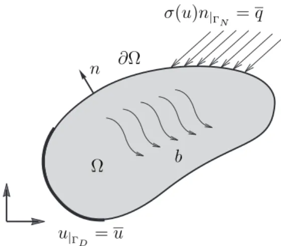
As mentioned before, the topological asymptotic expansion of the total potential energy associ-ated with the elasticity system into two spatial dimensions is obtained. Thus, the unperturbed shape functional is defined as:
ψ(χ) :=Jχ(u) = 1 2
!
Ω
σ(u)·∇su− !
Ω b·u−
!
ΓN
Figure 1: Topological derivative concept.
where the vector function uis the solution to the variational problem:
Findu∈U,such that !
Ω
σ(u)·∇sη = !
Ω b·η+
!
ΓN
q·η, ∀η∈V, (2.6)
withb a constant body force distributed in the domain,
σ(u) =C∇su (2.7)
the Cauchy stress tensor,
∇su= 1
2(∇u+∇
Tu) (2.8)
the linearized strain tensor and Cthe constitutive tensor given by
C= 2µI+λI⊗I, (2.9)
where I and I are the second and fourth identity tensors, respectively, µ and λ are the Lamé’s
coefficients, both considered constants everywhere. In the plane stress assumption we have
µ= E
2(1 +ν) and λ=
νE
1−ν2, (2.10)
while in plane strain assumption they are
µ= E
2(1 +ν) and λ=
νE
(1 +ν)(1−2ν), (2.11)
where E is the Young modulus and ν the Poisson ratio. The set of admissible displacements U
and the space of admissible displacements variations V are respectively defined as
U :={ϕ∈H1(Ω) :ϕ|ΓD =u} and V :={ϕ∈H1(Ω) :ϕ|ΓD = 0}. (2.12)
Here, ΓD and ΓN respectively are Dirichlet and Neumann boundaries such that∂Ω=ΓD∪ΓN
Figure 2: Mechanical problem defined in the unperturbed domain.
both assumed to be smooth enough. See details in Fig. 2. The strong system associated with the variational problem (2.6) is given by:
Find u, such that
divσ(u) = b inΩ,
σ(u) = C∇su,
u = u onΓD,
σ(u)n = q onΓN.
(2.13)
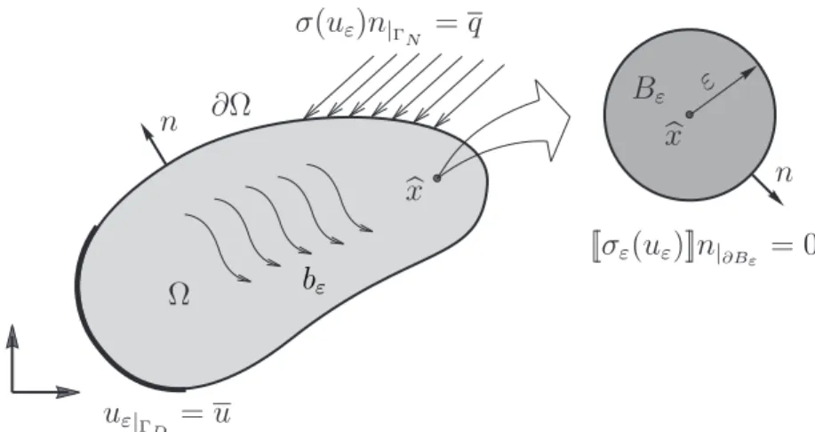
2.2 Perturbed problem
Now let us state the associate topologically perturbed problem. In this case, the total potential energy is given by
ψ(χε) :=Jχε(uε) =
1 2
!
Ω
σε(uε)·∇suε− !
Ω
bε·uε− !
ΓN
q·uε, (2.14)
where the vector function uε is the solution to the variational problem:
Finduε∈Uε, such that !
Ω
σε(uε)·∇sη= !
Ω
bε·η+ !
ΓN
q·η, ∀η∈Vε, (2.15)
with
σε(uε) =γεC∇suε and bε=γεb, (2.16) where γε is defined by (2.4). The setUε and the spaceVε are defined as
Uε:={ϕ∈U :!ϕ"= 0 on ∂Bε} and Vε:={ϕ∈V :!ϕ"= 0 on ∂Bε}, (2.17)
with the operator!ϕ"used to denote the jump of the functionϕon the boundary of the inclusion
∂Bε, namely !ϕ":=ϕ| Ω\Bε −
ϕ|B
Figure 3: Mechanical problem defined in the perturbed domain.
to the variational problem (2.15) reads:
Find uε, such that
divσε(uε) = bε in Ω,
σε(uε) = γεC∇suε,
uε = u onΓD,
σε(uε)n = q onΓN, !uε"
!σε(uε)"n = =
0 0
(
on∂Bε.
(2.18)
2.3 Existence of the topological derivative
The following result ensures the existence of the topological derivative associated with the prob-lem under analysis.
Lemma 1. Let u and uε be solutions to (2.6) and (2.15), respectively. Then we have that the estimate ,uε−u,H1(Ω)=O(ε) holds true.
Proof. We start by subtracting the variational problem (2.6) from (2.15) to obtain: !
Ω
(σε(uε)−σ(u))·∇sη = !
Ω
(bε−b)·η±
!
Ω
σε(u)·∇sη, ∀η∈Vε. (2.19)
From the above equation, we have: !
Ω
(σε(uε)−σε(u))·∇sη = − !
Ω
(σε(u)−σ(u))·∇sη+ !
Ω
(bε−b)·η. (2.20)
Recalling that: σε(uε) = σ(uε), bε =b in Ω\Bε and σε(uε) =γσ(uε), bε =γb in Bε, we have from (2.19):
!
Ω
σε(uε−u)·∇sη = (1−γ) !
Bε
σ(u)·∇sη+ (γ−1) !
Bε
By takingη=uε−uas test function in the above equation we obtain the following equality !
Ω
σε(uε−u)·∇s(uε−u) = (1−γ) !
Bε
σ(u)·∇s(uε−u) + (γ−1) !
Bε
b·(uε−u). (2.22)
From the Cauchy-Schwartz and Poincaré inequalities it follows that !
Ω
σε(uε−u)·∇s(uε−u) ≤ C1,σ(u),L2(Bε),∇
s(uε−u),
L2(Bε)+C2,b,L2(Bε),uε−u,L2(Bε)
≤ C3ε,∇s(uε−u),L2(Bε)+C4ε,uε−u,L2(Bε)
≤ C5ε,uε−u,H1(Bε)≤C6ε,uε−u,H1(Ω), (2.23)
where we have used the elliptic regularity of function u and the continuity of the functionb at the point "x∈Ω. Finally, from the coercivity of the bilinear form on the left-hand side of (2.22), namely
c,uε−u,2H1(Ω)≤
!
Ω
σε(uε−u)·∇s(uε−u), (2.24)
we obtain the result with the constant C =C6/cindependent of the small parameter ε.
2.4 The topological derivative formula
According to Novotny and Sokołowski (2013) the topological asymptotic expansion of the energy shape functional takes the form (see also Appendix 6):
ψ(χε(x)) =" ψ(χ)−πε2(Pγσ(u(x))" ·∇su(x) + (1" −γ)b(x)" ·u("x)) +o(ε2), (2.25)
where the polarization tensor Pγ is given by the following fourth order isotropic tensor
Pγ = 1
2 1−γ
1 +γα2 )
(1 +α2)I+ 1
2(α1−α2) 1−γ
1 +γα1 I⊗I
*
, (2.26)
with
α1 =
λ+µ
µ and α2 =
λ+ 3µ
λ+µ. (2.27)
Finally, in order to extract the main term of the above expansion, we choosef(ε) =πε2, which leads to the final formula for the topological derivative, namely:
T("x) =−Pγσ(u(x))" ·∇su(x)" −(1−γ)b(x)" ·u("x). (2.28)
Remark 2. Formally we can take the limit cases γ → 0 andγ → ∞. For γ →0, the inclusion leads to a void and the transmission condition on the interface of the inclusion degenerates to homogeneous Neumann boundary condition. In this case the polarization tensor is given by
P0 = λ+ 2µ
λ+µ )
I−µ−λ
4µ I⊗I *
In addition, for γ → ∞, the elastic inclusion leads to a rigid one and the polarization tensor is stated as
P∞ = −λ+ 2µ
λ+ 3µ )
I+ µ−λ
4(λ+µ)I⊗I *
. (2.30)
In the case of plane strain linear elasticity, the above formulas are written as
P0= 1−ν
2 +
4I+1−4ν
1−2νI⊗I
,
and P∞=−(1−ν)
+ 1 3−4νI+
1−4ν
2(3−4ν)I⊗I ,
, (2.31)
while in the case ofplane stress linear elasticity the formulas are explicitly given by
P0 = 1
1 +ν
+
2I− 1−3ν
2(1−ν)I⊗I ,
and P∞=− 1
3−ν
+
2I+ 1−3ν
2(1 +ν)I⊗I ,
. (2.32)
Remark 3. The polarization tensor Pγ and theirs associated particular representations lead
to isotropic fourth order tensors because we are dealing with circular inclusions as topological perturbations. For arbitrary shaped inclusions the reader may refer to the book by Ammari and Kang (2007), for instance. On the other hand, there are two main advantages in using circular inclusions in the context of topology optimization, which are:
• The associated topological derivative is given by a closed formula depending on the solution to the original unperturbed problem.
• There are optimality conditions rigorously derived in Amstutz (2011), allowing for use the topological derivative together with a level-set domain representation method as a steepest-descent direction in a topology optimization algorithm (Amstutz and Andrä (2006)).
3
THE TOPOLOGY OPTIMIZATION PROBLEMWe consider the compliance topology optimization of structures subject to multiple load-cases under volume constraint. Therefore, the topology optimization problem can be stated as
P1 : Minimize
Ω⊂D FΩ(ui) =−
NLC
-i=0
Jχ(ui),
subject to |Ω|≤M,
(3.1)
where NLC is the number of load-cases, M > 0 is the required volume at the end of the opti-mization process andui is solution to:
• for i= 0
Findu0, such that
divσ(u0) = ρb inD,
σ(u0) = ρC∇su0,
u0 = 0 onΓD,
σ(u0)n = 0 onΓN;
Figure 4: Computational domain.
• for i= 1, . . . ,NLC
Find ui, such that
divσ(ui) = 0 inD,
σ(ui) = ρC∇sui,
ui = 0 onΓD,
σ(ui)n = qi onΓN.
(3.3)
Here, D is used to denote a hold-all domain. In order to simplify the numerical implementation we consider that the elastic bodyD is decomposed into two sub-domainsΩand ω. The domain Ω = D \ω represents the elastic part while ω ⊂ D is filled with a very complacent material, used to mimic voids. See the sketch in Fig. 4. This procedure allows us to work in a fixed computational domain. Therefore, we define a characteristic function of the form
x%→χ(x) = #
1, if x∈D,
0, if x∈R2\ D. (3.4)
In addition, we introduce a piecewise constant functionρ, such that
ρ(x) = #
1, if x∈Ω,
ρ0, if x∈ω, (3.5)
with 0 < ρ0 / 1 used to mimic voids. That is, the original optimization problem, where the structure itself consists of the domainΩof given elastic properties and the remaining empty part
ω, is approximated by means of the two-phase material distribution given by (3.5) overDwhere the empty region ω is filled by a material (the soft phase) with Young’s modulus, ρ0E, much lower than the given Young’s modulus, E, of the structure material (the hard phase).
3.1 Augmented lagrangian
The volume constraint is imposed through the Augmented Lagrangian Method. It consists in transform the inequality constraint in Problem P1given by (3.1) into an equality by introducing a slack function s, namely
P2 :
Minimize
Ω⊂D FΩ(ui) =−
NLC
-i=0
Jχ(ui),
subject tohΩ(s) =gΩ+s2,
where gΩ = (|Ω|−M)/M. Note that for an optimal value s=s∗ the equivalence P2≡P1holds true. Let us introduce two Lagrange multipliers α andβ. Then, the ProblemP2 in (3.6) can be rewritten as
P3 :
Minimize
Ω⊂D F.Ω(ui) =−
NLC
-i=0
Jχ(ui) +αhΩ(s) +
β
2hΩ(s) 2,
subject tohΩ(s) =gΩ+s2.
(3.7)
Note that if hΩ(s∗) = 0, then P3 ≡P2 ≡ P1. Thus, let us minimize (3.7) with respect to the slack function s, namely
#
αh%Ω(s) +βhΩ(s)h%Ω(s) = 0, h%
Ω(s) = 2s.
(3.8)
Then, s= 0 or s2=−(α/β+gΩ). Therefore
(s∗)2 = max{0,−(α/β+gΩ)}. (3.9)
It follows that:
hΩ(s∗) = gΩ+ max{0,−(α/β+gΩ)}
= max{gΩ,−α/β}:=gΩ+. (3.10)
Finally, by settings=s∗ we haveP4≡P3≡P2≡P1, that allows us to rewrite the constrained ProblemP1, given by (3.1), in its equivalent unconstrained form, namely
P4 : /
Minimize
Ω⊂D F.Ω(ui) =−
NLC
-i=0
Jχ(ui) +αg+Ω +
β
2(g +
Ω)2 . (3.11)
In addition we have thatβ, the parameter associated to the quadratic term, controls the updating of the parameter α, which is associated with the linear term. Therefore, we can specify the required volume fraction at the final of the optimization process by solving the following recursive formula for the parameterα:
α0 = 0
αn+1= max{0,αn+βgΩ}, (3.12)
where β > 0 is a fixed number. This updating process shall be repeated until the volume constraint is reached, as can be seen in Algorithm 1 at the end of Section 4.
3.2 Topological derivative
since the topological derivative satisfies the basic rules of the Differential Calculus (Novotny and Sokołowski (2013)) and taking into account the linearity of the elasticity problem, we have
T("x) =
NLC
-i=0
(P0σ(ui("x))·∇sui(x) +" bi·ui)−max{0,α+βgΩ}, ifx"∈Ω,
NLC
-i=0
(P∞σ(ui("x))·∇sui("x)−bi·ui) + max{0,α+βgΩ}, ifx"∈ω.
(3.13)
Therefore, the topological derivative associated with Problem P4 is obtained as a sum of the topological derivatives for each load-case together with the topological derivative of the aug-mented Lagrangian terms, which is trivially obtained by considering the limit cases in Remark 2.
4
THE TOPOLOGY OPTIMIZATION ALGORITHMIn this section a topology optimization algorithm based on the topological derivative together with a level-set domain representation method is presented. It has been proposed by Amstutz and Andrä (2006) and consists basically in looking for a local optimality condition for the mini-mization problem (3.11), written in terms of the topological derivative and a level-set function. Therefore, the elastic partΩas well as the complacent materialωare characterized by a level-set functionΨ∈L2(D)of the form:
Ω={Ψ(x)<0a.e. inD} and ω ={Ψ(x) >0a.e. in D}, (4.1)
whereΨvanishes on the interface ∂ω. A local sufficient optimality condition for Problem (3.11), under the considered class of domain perturbation given by circular inclusions, can be stated as (Amstutz (2011))
T(x)>0 ∀x∈D. (4.2)
Therefore, let us define the quantity
g(x) := #
−T(x), if Ψ(x)<0,
T(x), if Ψ(x)>0, (4.3)
allowing for rewrite the condition (4.2) in the following equivalent form #
g(x)<0, if Ψ(x)<0,
g(x)>0, if Ψ(x)>0. (4.4)
We observe that (4.4) is satisfied wether the quantity g coincides with the level-set function Ψ up to a strictly positive number, namely ∃τ >0 :g=τΨ, or equivalently
θ:= arccos 0
2g,Ψ3L2(D)
,g,L2(D),Ψ,L2(D)
1
= 0, (4.5)
Algorithm 1:The topology design algorithm
input :NLC,D,Ψ0,M,α0,β,2κ,2θ,2M
output: The optimal topology Ω' 1 n←0;
2 Ωn←Ψn;Ept←0; 3 for i←0 : NLC do 4 if i= 0 then
5 solve (3.2);
6 else
7 solve (3.3);
8 end if
9 Ept ←Ept+Jχ(ui); 10 end for
11 ComputeF.Ω
n according to (3.11);
12 ComputeT("x) using (3.13); 13 Computegn according to (4.3);
14 θn←arccos
+
&gn,Ψn' (gn(L2(D)(Ψn(L2(D)
, ;
15 Ψold←Ψn; F.old←F.Ω
n; F.new ←F.old+ 1; κ←1;
16 while F.new >F.old do
17 Ψnew← 1
sinθn
+
sin((1−κ)θn)Ψold+ sin(κθn)(gn(gn
L2(D)
, ;
18 Ψn←Ψnew; 19 execute lines 2-11;
20 F.new ←F.Ω
n;
21 κ←κ/2;
22 end while
23 if κ<2κ then
24 try a mesh refinement;
25 Ψn+1 ←Ψn; n←n+ 1; 26 go to line 2;
27 else if θn>2θ then 28 Ψn+1 ←Ψn; n←n+ 1; 29 go to line 2;
30 else
31 if |1−|Ωn|/M|>2M then
32 compute αn+1 according to (3.12);
33 Ψn+1 ←Ψn; n←n+ 1; 34 go toline 2;
35 else
36 Ω'←Ψn;
37 stop;
38 end if
Let us now explain the algorithm. We start by choosing an initial level-set function Ψ0 ∈ L2(D). In a generic iteration n, we compute function gn associated with the level-set function
Ψn∈L2(D). Thus, the new level-set functionΨn+1 is updated according to the following linear combination between the functionsgn and Ψn
Ψ0 ∈L2(D),
Ψn+1 = 1 sinθn
0
sin((1−κ)θn)Ψn+ sin(κθn) gn
,gn,L2(D)
1
∀n∈N, (4.6)
where θn is the angle between gn and Ψn, and κ is a step size determined by a linear-search
performed in order to decrease the value of the objective functionF.Ωn, withΩn used to denote the elastic part associated toΨn. The process ends when the conditionθn≤2θ and at the same time the required volume|1−|Ωn|/M|≤2M are satisfied in some iteration, where2θand2M are
given small numerical tolerances. In particular, we can choose
Ψ0∈S={x∈L2(D);,x,L2(D)= 1}, (4.7)
and by construction Ψn+1 ∈ S, ∀n∈ N. If at some iteration n the linear-search step size κ is found to be smaller then a given numerical tolerance2κ >0and the optimality condition is not satisfied, namelyθn>2θ, then a uniform mesh refinement of the hold all domainDis carried out and the iterative process is continued. The resulting topology design algorithm is summarized in a pseudo-code format, see Algorithm 1.
5
NUMERICAL EXAMPLESSince we are dealing with multiple load-cases, two situations denoted by C1 and C2 are con-sidered. In the first case (C1), the loads are applied simultaneously (single load-case) and the associated topological derivative is evaluated. On the other hand, in the second case (C2), the loads are applied separately (multiple load-cases) and the resulting topological derivative is obtained as a sum of the topological derivatives associated with each load-case.
In all numerical examples the stopping criterion, the optimality threshold and the tolerance of the volume requirement are given respectively by2κ = 10−3,2θ = 1o and2M = 1%. The angle
θhas converged to a value smaller than1o, namely, the optimality condition has been satisfied in all cases up to a small numerical tolerance. Furthermore, the mechanical problem is discretized into linear triangular finite elements and three steps of uniform mesh refinement were performed during the iterative process.
We assume that in the first three examples the structures are under plane strain assumption while in the last two examples the structures are under plane stress assumption. Finally, the material property threshold is set asρ0 = 10−4, while the Young’s modulus is given byE= 1.0.
5.1 Example 1
Figure 5: Example 1: initial guess and boundary conditions.
The Poisson ratio is given by ν = 0.3. The required volume fraction is set as M = 50%, while the parameters of the augmented Lagrangian method are given by α0 = 0.0 andβ = 10.0. The final topologies are obtained after 41 and 31 iterations for the cases C1 and C2, respectively, as shown in Figs. 6(a) and 6(b). We observe that the obtained result for multiple load-cases is feasible while the result for single load-case doesn’t make sense from physical point of view.
(a) single load-case (b) multiple load-cases
Figure 6: Example 1: obtained results.
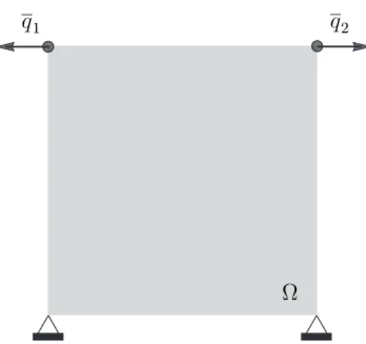
5.2 Example 2
Figure 7: Example 2: initial guess and boundary conditions.
The required volume fraction is given by M = 50% and the parameters of the augmented Lagrangian method are α0 = 0.0 and β = 10.0. The Poisson ratio is set as ν = 0.3. The final results are obtained with 27and 28iterations for the casesC1andC2, respectively, as shown in Figs. 8(a) and 8(b).
(a) single load-case (b) multiple load-cases
Figure 8: Example 2: obtained results.
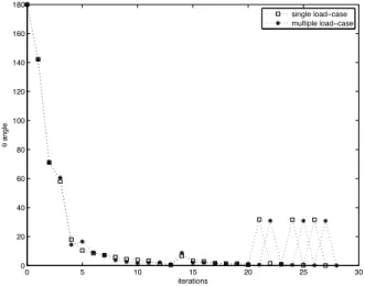
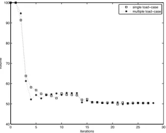
The convergence of theθn angle and volume fraction, for the cases C1and C2, are respectively presented in Figs. 9 and 10. The jumps on the values ofθn in the graph of Fig. 9 are due to the
mesh refinement.
0 5 10 15 20 25 30
0 20 40 60 80 100 120 140 160 180
iterations
!
angle
single load−case multiple load−case
0 5 10 15 20 25 30 40
50 60 70 80 90 100
iterations
volume
single load−case multiple load−case
Figure 10: Example 2: convergence history of the volume fraction.
The multiple load-cases C2allow for a more realistic combination of the applied forces resulting in topologies that best satisfy the conditions of the problem. Thus in the next three examples only the results for multiple load-cases are presented.
5.3 Example 3
This example simulates the design of a barrage. The hold-all domain is a square of size 1×1 clamped on its bottom edge, as illustrated by Fig. 11(a). The hydrostatic pressure is represented by a distributed load on the left-hand side of the barrage. There is also a constant body force b= (0.0,−0.1) acting in the whole domain. The initial mesh is uniform with 1600 elements and 841 nodes.
(a) initial guess and boundary conditions (b) obtained result
Figure 11: Example 3: barrage design.
5.4 Example 4
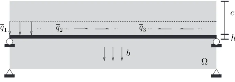
Let us consider now a bridge design. The hold-all domain is given by a rectangle of size 3×1 supported on the two opposites bottom corners. The bridge is submitted to three uniformly distributed traffic loading q
1 = (0.0,−10.0), q2 = (1.0,0.0) and q3 = (−1.0,0.0) applied on the dark strip of height h = 0.05 positioned at the distance c = 0.45 from the top of the hold-all domain. This strip represents the road, which is simply supported on their opposites bottom corners, and therefore remains unchanged throughout the optimization process. We also consider a body force given by b= (0.0,−0.4). See the sketch in Fig. 12. The domain is discretized into a uniform mesh with 4800 elements and2481 nodes.
Figure 12: Example 4: initial guess and boundary conditions.
The parameters of the augmented Lagrangian method are given by α0 = 0.0and β = 1.0, while the required volume fraction is set as M = 30%. The Poisson ratio is given by ν = 0.3. The final topology is obtained after28 iterations and can be seen in Fig. 13.
Figure 13: Example 4: obtained result.
5.5 Example 5
(a) initial guess and boundary conditions (b) obtained result
Figure 14: Example 5: alloy wheel design.
The Poisson ratio is set asν = 0.3, while the required volume fraction is M = 73%, where the parameters of the augmented Lagrangian method are given byα0 = 0.0 andβ= 12.0. The final topology is obtained with just20 iterations and can be seen in Fig. 14(b).
6
CONCLUSIONIn this paper the topological derivative was applied in the context of topology optimization of structures subject to multiple load-cases. The structural compliance into two spatial dimensions was minimized under volume constraint. Since the topological derivative obeys the basic rules of the Differential Calculus, the topological sensitivity of a multi-objective shape functional was obtained as a sum of the topological derivatives associated with each load-case. In addition, the obtained sensitivity has been used as a steepest-descent direction similar to any gradient-based method. In particular, a fixed-point algorithm based on the topological derivative together with a level-set domain representation method has been presented, which converges to a local optimum. The resulting algorithm has been summarized in a pseudo-code format easy to implement and several finite element-based examples of structural optimization were presented. Finally, for the reader convenience, the topological asymptotic analysis of the total potential energy with respect to the nucleation of a small circular inclusion was developed in a simplified and pedagogical manner by using standard arguments from the Analysis. Therefore, we believe that this paper would be useful for the readers interested on the mathematical aspects of topological asymptotic analysis as well as on applications of topological derivatives in structural optimization.
Acknowledgements
APPENDIX A ASYMPTOTIC ANALYSIS
In this appendix the proof of the result (2.25) together with the estimation for the remainder on the topological asymptotic expansion are presented. The results are derived by using simple arguments from the Analysis.
A.1 Polarization tensor in elasticity
In order to calculate the difference between the functionalsψ(χ)and ψ(χε), respectively defined through (2.5) and (2.14), we start by taking η = uε −u as test function in the variational problems (2.6) and (2.15), leading respectively to
1 2
!
Ω
σ(u)·∇su = 1 2
!
Ω
σ(u)·∇suε−1 2
!
Ω
b·(uε−u)− 1 2
!
ΓN
q·(uε−u), (.1)
1 2
!
Ω
σε(uε)·∇suε = 1 2
!
Ω
σε(uε)·∇su+ 1 2
!
Ω
bε·(uε−u)− 1 2
!
ΓN
q·(uε−u). (.2)
So that the shape functionals ψ(χ) andψ(χε)can be rewritten as:
ψ(χ) = 1 2
!
Ω
σ(uε)·∇su−1 2
!
Ω
b·(uε+u)−1 2
!
ΓN
q·(uε+u), (.3)
ψ(χε) = 1 2
!
Ω
σε(uε)·∇su− 1 2
!
Ω
bε·(uε+u)−1 2
!
ΓN
q·(uε+u). (.4)
Now, after subtracting (.3) from (.4) we obtain:
ψ(χε)−ψ(χ) = 1 2
!
Ω
σε(uε)·∇su−1 2
!
Ω
σ(uε)·∇su−1 2
!
Ω
bε·(uε+u) +1 2
!
Ω
b·(uε+u)
= 1 2
0!
Ω\Bε
σ(uε)·∇su+ !
Bε
γσ(uε)·∇su 1
− 1
2 0!
Ω\Bε
σ(uε)·∇su
+ !
Bε
σ(uε)·∇su ,
−1
2 0!
Ω\Bε
b·(uε+u) + !
Bε
γb·(uε+u) 1
+ 1 2
0!
Ω\Bε
b·(uε+u) + !
Bε
b·(uε+u) 1
= 1 2
!
Bε
(γ−1)σ(uε)·∇su−1 2
!
Bε
(1−γ)b·(uε+u)
= −1−γ 2γ
!
Bε
σε(uε)·∇su− 1−γ
2 !
Bε
b·(uε+u). (.5)
Note that the resulting terms of the difference between ψ(χ) and ψ(χε) are given by integrals concentrated over the inclusion Bε.
Now, in order to evaluate the limit in (2.3), we need to know the behavior of the functionuε with respect toε→0. Thus, let us introduce the following ansätz:
where wε(x) is the solution to an auxiliary exterior problem and uε(x)˜ is the remainder. After applying the operator σε in (.6), we obtain
σε(uε(x)) =σε(u("x)) +γε∇σ(u(ξ))(x−x) +" σε(wε(x)) +σε(˜uε(x)), (.7) where σ(u(x)) has been expanded in Taylor series around the pointx"and ξ is used to denote a point betweenx and "x. From the transmission condition on the interface ∂Bε, we have
!σε(uε)"n= 0 ⇒ (σ(uε)|Ω\Bε−γσ(uε)|Bε)n= 0. (.8)
Therefore, according to Fig. 3,n= (x−"x)/ε, and
!σε(uε)"n = (1−γ)σ(u(x))n" +ε(1−γ)(∇σ(u(ξ))n)n
+ !σε(wε(x))"n+!σε(˜uε(x))"n= 0. (.9) Thus, we can chooseσε(wε) such that:
!σε(wε)"n=−(1−γ)σ(u(x))n" on ∂Bε (.10) and by a changing variables, we write
wε(x) =εw(x/ε) and y =x/ε, (.11)
which implies ∇yw(y) =ε∇w(x/ε). In the new variable the following exterior problem is
con-sidered:
Findσy(w),such that
divy(σy(w)) = 0 inR2,
σy(w) → 0 at∞,
(γσy(w)|R2\B1 −σy(w)|B1)n = "u,
(.12)
withu"=−(1−γ)σ(u("x))n. The above boundary value problem admits an explicit solution. In fact, since the tress σy(w) is uniform inside the inclusion, it can be written in a compact form making use of the Eshelby’s Theorem (Eshelby (1957, 1959)):
σy(w) =Tσ(u(x))," (.13)
where Tis a fourth order isotropic tensor written as
T= γ(1−γ)
2(1 +γα2) )
2α2I+
α1−α2 1 +γα1
I⊗I *
, (.14)
with the constants α1 and α2 given by (2.27).
Now we can construct σε(.uε)in such a way that it compensates the discrepancies introduced by the higher-order terms in εas well as by the boundary-layerσy(w) on the exterior boundary
∂Ω. It means that the remainder .uε must be solution to the following boundary value problem:
Find .uε, such that
div(σε(uε)). = 0 inΩ,
σε(.uε) = γεC∇s.uε .
uε = −εw onΓD,
σε(.uε)n = −εσ(w)n onΓN, !u.ε"
!σε(.uε)"n = =
0
εh (
on∂Bε,
withh =−(1−γ)(∇σ(u(ξ))n)n. Moreover, we can obtain an estimate for the remainder uε. of the form O(ε). In fact, before proceeding, let us state the following result, which can be found in the book Novotny and Sokołowski (2013) in its optimal version, namely O(ε2):
Lemma 4. Let .uε be solution to (.15). Then, the following estimate holds true:
,uε,. H1(Ω)≤Cε, (.16)
with the constant C independent of the small parameter ε.
Proof. From the expansion for uε and making use of the triangular inequality, we can write
|.uε(x)|H1(Ω) = |uε(x)−u(x)−εw(x/ε)|H1(Ω)
≤ |uε(x)−u(x)|H1(Ω)+ε|w(x/ε)|H1(Ω)
≤ ,uε(x)−u(x),H1(Ω)+ε|w(y)|H1(R2)
≤ C1ε, (.17)
where we have used the change of variables (.11), the equivalence between the semi-norm|·|H1(Ω)
and the norm ,·,H1(Ω) and the estimate in Lemma 1. Finally, the result comes out from the
Poincaré inequality.
Now, we have all the necessary elements to evaluate the integral in (.5). In fact, after replacing (.6) into (.5) and takin into account (.11) we have:
ψ(χε)−ψ(χ) = − 1−γ
2γ
+!
Bε
γσ(u)·∇su+ !
Bε
σy(w)·∇su+
!
Bε
σε(u.ε)·∇su ,
− 1−γ
2 +!
Bε
2b·u+ !
Bε
b·(εw+uε). ,
= −πε21−γ
2 σ(u("x))·∇
su(
"
x)−πε2(1−γ)b·u("x)−1−γ 2γ
!
Bε
σy(w)·∇su
− 1−γ
2γ
+!
Bε
σy(w)·(∇su(x)− ∇su(x)) +" !
Bε
σε(.uε)·∇su ,
− 1−γ
2 +!
Bε
σ(u(x))·∇su(x)−σ(u(x))" ·∇su(x) +" !
Bε
b·(εw+uε). ,
= −πε21−γ
2 σ(u("x))·∇
su(
"
x)−πε2(1−γ)b·u("x)
− 1−γ
2γ
!
Bε
σy(w)·∇su+ 5
-i=1
Ei(ε), (.18)
where the remainders Ei(ε) =o(ε2), fori= 1, ...,5, as shown in Section 6. Thus the topological
asymptotic expansion of the energy shape functional takes the form:
ψ(χε(x)) =" ψ(χ)−πε21−γ
2γ (γI+T)σ(u(x))" ·∇
su(
"
x)−πε2(1−γ)b·u(x) +" o(ε2). (.19)
By defining the function f(ε) =πε2 and the polarization tensor as:
Pγ = 1−γ
2γ (γI+T)
= 1−γ
2(1 +γα2) )
(1 +α2)I+ 1
2(α1−α2) 1−γ
1 +γα1 I⊗I
*
it follows that the topological derivative of the shape functional ψ evaluated at the arbitrary point "x∈Ωis given by
T(x) =" −Pγσ(u(x))" ·∇su(x)" −(1−γ)b·u(x)." (.21)
Note that both tensors Pγ and T are isotropic because we are dealing with circular inclusions.
For arbitrary shaped inclusions the reader may refer to Ammari and Kang (2007).
A.2 Estimation of the remainders
The first remainder term E1(ε) is estimated as follow:
E1(ε) = !
Bε
(ϕ(x)−ϕ("x))
≤ ,1,L2(Bε),ϕ(x)−ϕ("x),L2(Bε)
≤ C0ε,x−x," L2(Bε)
≤ C1ε3=o(ε2), (.22)
with ϕ := σ(u) ·∇su, where we have used the Cauchy-Schwartz inequality and the elliptic
regularity ofu. From the fact that the stressσy(w)is uniform inside the inclusion and using the same arguments, we have the following estimate for the second remainder term:
E2(ε) = !
Bε
σy(w)·(∇su(x)− ∇su(x))"
≤ ,σy(w),L2(B
ε),∇
su(x)− ∇su(
" x),L2(B
ε)
≤ C2ε,x−x," L2(B
ε)
≤ C3ε3 =o(ε2). (.23)
Once again, from the Cauchy-Schwartz inequality and the elliptic regularity of u we have the estimate bellow for the third remainder
E3(ε) = !
Bε
σ(.uε)·∇su= !
Bε
∇s.uε·σ(u)
≤ ,∇s.uε,L2(B
ε),σ(u),L2(Bε)
≤ C4ε,∇suε,. L2(Bε). (.24)
In addition, note that the right-hand side of (.15) depends explicitly on the small parameter ε. Since this problem is linear and in view of Lemma 4, we can writeuε. =εϕ0. Therefore
E3(ε) ≤ C4ε2,∇sϕ0,L2(B
ε)
≤ C5ε3 =o(ε2), (.25)
Now, using again the elliptic regularity ofu and the continuity of function bat the point "x∈Ω, the remainder term E4 is estimate as follows
E4 =
!
Bε
b·(u(x)−u(x))"
≤ ,b,L2(Bε),u(x)−u("x),L2(Bε)
≤ C6ε,x−x," L2(B
ε)
Finally, the last remainder E5(ε) is defined as:
E5(ε) = !
Bε
b·(εw+uε) =. !
Bε
b·(uε−u). (.27)
Therefore, from the Cauchy-Schwartz inequality and Lemma 1 we obtain !
Bε
b·(uε−u) ≤ ,b,L2(B
ε),uε−u,L2(Bε)
≤ C8ε,uε−u,L2(Bε), (.28)
where we have considered the fact that the function b is assumed to be constant in the neigh-borhood of the point"x∈Ω. By making use of the Hölder inequality together with the Sobolev embbeding theorem, there is
,uε−u,L2(B
ε) ≤
0)!
Bε
(|uε−u|2)p
*1/p)!
Bε
1q
*1/q11/2
= π1/2qε1/q
)!
Bε
|uε−u|2p
*1/2p
= π1/2qε1/q,uε−u,L2p(B
ε)
≤ C9εδ,uε−u,H1(Ω), (.29)
where1/p+ 1/q = 1, withq >1, and δ= 1/q. Therefore !
Bε
b·(uε−u) ≤ C10ε1+δ,uε−u,H1(Ω)
≤ C11ε2+δ=o(ε2), (.30)
where we have used Lemma 1 and the fact that 0<δ<1.
References
Allaire, G., de Gournay, F., Jouve, F., and Toader, A. M. Structural optimization using topo-logical and shape sensitivity via a level set method. Control and Cybernetics, 34(1):59–80, 2005.
Allaire, G., Jouve, F., and Van Goethem, N. Damage and fracture evolution in brittle materials by shape optimization methods. Journal of Computational Physics, 230(12):5010–5044, 2011.
Ammari, H. and Kang, H. Polarization and moment tensors with applications to inverse problems and effective medium theory. Applied Mathematical Sciences vol. 162. Springer-Verlag, New York, 2007.
Ammari, H., Kang, H., Lee, H., and Lim, J. Boundary perturbations due to the presence of small linear cracks in an elastic body. Journal of Elasticity, páginas 1–17, 2014.
Amstutz, S. A penalty method for topology optimization subject to a pointwise state constraint. ESAIM: Control, Optimisation and Calculus of Variations, 16(03):523–544, 2010.
Amstutz, S. Analysis of a level set method for topology optimization. Optimization Methods and Software, 26(4-5):555–573, 2011.
Amstutz, S. and Andrä, H. A new algorithm for topology optimization using a level-set method. Journal of Computational Physics, 216(2):573–588, 2006.
Amstutz, S., Giusti, S. M., Novotny, A. A., and de Souza Neto, E. A. Topological derivative for multi-scale linear elasticity models applied to the synthesis of microstructures. International Journal for Numerical Methods in Engineering, 84:733–756, 2010.
Amstutz, S., Horchani, I., and Masmoudi, M. Crack detection by the topological gradient method. Control and Cybernetics, 34(1):81–101, 2005.
Amstutz, S. and Novotny, A. A. Topological optimization of structures subject to von Mises stress constraints. Structural and Multidisciplinary Optimization, 41(3):407–420, 2010.
Amstutz, S., Novotny, A. A., and de Souza Neto, E. A. Topological derivative-based topology optimization of structures subject to Drucker-Prager stress constraints. Computer Methods in Applied Mechanics and Engineering, 233–236:123–136, 2012.
Auroux, D., Masmoudi, M., and Belaid, L. Image restoration and classification by topologi-cal asymptotic expansion. In: Variational formulations in mechanics: theory and applications, Barcelona, Spain, 2007.
Belaid, L. J., Jaoua, M., Masmoudi, M., and Siala, L. Application of the topological gradient to image restoration and edge detection. Engineering Analysis with Boundary Element, 32(11): 891–899, 2008.
Bojczuk, D. and Mróz, Z. Topological sensitivity derivative and finite topology modifications: application to optimization of plates in bending. Structural and Multidisciplinary Optimization, 39(1):1–15, 2009.
Burger, M., Hackl, B., and Ring, W. Incorporating topological derivatives into level set methods. Journal of Computational Physics, 194(1):344–362, 2004.
Canelas, A., Laurain, A., and Novotny, A. A. A new reconstruction method for the inverse potential problem. Journal of Computational Physics, páginas 1–26, 2014.
Canelas, A., Novotny, A. A., and Roche, J. R. A new method for inverse electromagnetic casting problems based on the topological derivative. Journal of Computational Physics, 230:3570–3588, 2011.
de Faria, J. R. and Novotny, A. A. On the second order topologial asymptotic expansion. Structural and Multidisciplinary Optimization, 39(6):547–555, 2009.
Eshelby, J. D. The determination of the elastic field of an ellipsoidal inclusion, and related problems. Proceedings of the Royal Society: Section A, 241:376–396, 1957.
Eshelby, J. D. The elastic field outside an ellipsoidal inclusion, and related problems. Proceedings of the Royal Society: Section A, 252:561–569, 1959.
Feijóo, G. R. A new method in inverse scattering based on the topological derivative. Inverse Problems, 20(6):1819–1840, 2004.
Feijóo, R. A., Novotny, A. A., Taroco, E., and Padra, C. The topological derivative for the Poisson’s problem. Mathematical Models and Methods in Applied Sciences, 13(12):1825–1844, 2003.
Garreau, S., Guillaume, P., and Masmoudi, M. The topological asymptotic for PDE systems: the elasticity case. SIAM Journal on Control and Optimization, 39(6):1756–1778, 2001.
Giusti, S. M., Novotny, A. A., and de Souza Neto, E. A. Sensitivity of the macroscopic response of elastic microstructures to the insertion of inclusions. Proceeding of the Royal Society A: Mathematical, Physical and Engineering Sciences, 466:1703–1723, 2010a.
Giusti, S. M., Novotny, A. A., de Souza Neto, E. A., and Feijóo, R. A. Sensitivity of the macroscopic elasticity tensor to topological microstructural changes. Journal of the Mechanics and Physics of Solids, 57(3):555–570, 2009a.
Giusti, S. M., Novotny, A. A., de Souza Neto, E. A., and Feijóo, R. A. Sensitivity of the macro-scopic thermal conductivity tensor to topological microstructural changes. Computer Methods in Applied Mechanics and Engineering, 198(5–8):727–739, 2009b.
Giusti, S. M., Novotny, A. A., and Padra, C. Topological sensitivity analysis of inclusion in two-dimensional linear elasticity. Engineering Analysis with Boundary Elements, 32(11):926–935, 2008.
Giusti, S. M., Novotny, A. A., and Sokołowski, J. Topological derivative for steady-state or-thotropic heat diffusion problem. Structural and Multidisciplinary Optimization, 40(1):53–64, 2010b.
Guzina, B. B. and Bonnet, M. Small-inclusion asymptotic of misfit functionals for inverse prob-lems in acoustics. Inverse Problems, 22(5):1761–1785, 2006.
Hintermüller, M. Fast level set based algorithms using shape and topological sensitivity. Control and Cybernetics, 34(1):305–324, 2005.
Hintermüller, M. and Laurain, A. Electrical impedance tomography: from topology to shape. Control and Cybernetics, 37(4):913–933, 2008.
Hintermüller, M. and Laurain, A. Multiphase image segmentation and modulation recovery based on shape and topological sensitivity. Journal of Mathematical Imaging and Vision, 35: 1–22, 2009.
Hlaváček, I., Novotny, A. A., Sokołowski, J., and Żochowski, A. On topological derivatives for elastic solids with uncertain input data. Journal of Optimization Theory and Applications, 141 (3):569–595, 2009.
Jackowska-Strumiłło, L., Sokołowski, J., Żochowski, A., and Henrot, A. On numerical solution of shape inverse problems. Computational Optimization and Applications, 23(2):231–255, 2002.
Khludnev, A. M., Novotny, A. A., Sokołowski, J., and Żochowski, A. Shape and topology sensitivity analysis for cracks in elastic bodies on boundaries of rigid inclusions. Journal of the Mechanics and Physics of Solids, 57(10):1718–1732, 2009.
Kobelev, V. Bubble-and-grain method and criteria for optimal positioning inhomogeneities in topological optimization. Structural and Multidisciplinary Optimization, 40(1-6):117–135, 2010.
Larrabide, I., Feijóo, R. A., Novotny, A. A., and Taroco, E. Topological derivative: a tool for image processing. Computers & Structures, 86(13–14):1386–1403, 2008.
Leugering, G. and Sokołowski, J. Topological derivatives for elliptic problems on graphs. Control and Cybernetics, 37:971–998, 2008.
Lewinski, T. and Sokołowski, J. Energy change due to the appearance of cavities in elastic solids. International Journal of Solids and Structures, 40(7):1765–1803, 2003.
Masmoudi, M., Pommier, J., and Samet, B. The topological asymptotic expansion for the Maxwell equations and some applications. Inverse Problems, 21(2):547–564, 2005.
Nazarov, S. A. and Sokołowski, J. Asymptotic analysis of shape functionals. Journal de Mathé-matiques Pures et Appliquées, 82(2):125–196, 2003a.
Nazarov, S. A. and Sokołowski, J. Self-adjoint extensions of differential operators in application to shape optimization. Comptes Rendus Mecanique, 331:667–672, 2003b.
Nazarov, S. A. and Sokołowski, J. Singular perturbations in shape optimization for the Dirichlet laplacian. C. R. Mecanique, 333:305–310, 2005.
Nazarov, S. A. and Sokołowski, J. Self-adjoint extensions for the Neumann laplacian and appli-cations. Acta Mathematica Sinica (English Series), 22(3):879–906, 2006.
Nazarov, S. A. and Sokołowski, J. On asymptotic analysis of spectral problems in elasticity. Latin American Journal of Solids and Structures, 8:27–54, 2011.
Novotny, A. A., Feijóo, R. A., Padra, C., and Taroco, E. Topological sensitivity analysis. Com-puter Methods in Applied Mechanics and Engineering, 192(7–8):803–829, 2003.
Novotny, A. A., Feijóo, R. A., Padra, C., and Taroco, E. Topological derivative for linear elastic plate bending problems. Control and Cybernetics, 34(1):339–361, 2005.
Novotny, A. A. and Sokołowski, J. Topological derivatives in shape optimization. Interaction of Mechanics and Mathematics. Springer, 2013.
Novotny, A. A., Sokołowski, J., and de Souza Neto, E. A. Topological sensitivity analysis of a multi-scale constitutive model considering a cracked microstructure. Mathematical Methods in the Applied Sciences, 33(5):676–686, 2010.
Sokołowski, J. and Żochowski, A. On the topological derivative in shape optimization. SIAM Journal on Control and Optimization, 37(4):1251–1272, 1999.
Sokołowski, J. and Żochowski, A. Optimality conditions for simultaneous topology and shape optimization. SIAM Journal on Control and Optimization, 42(4):1198–1221, 2003.
Sokołowski, J. and Żochowski, A. Modelling of topological derivatives for contact problems. Numerische Mathematik, 102(1):145–179, 2005.
Turevsky, I., Gopalakrishnan, S. H., and Suresh, K. An efficient numerical method for computing the topological sensitivity of arbitrary-shaped features in plate bending. International Journal for Numerical Methods in Engineering, 79(13):1683–1702, 2009.