! ""
The primary function of a vehicle suspension system is to isolate the road excitations experienced by the tyres from being transmitted to the passengers. In this paper, a suitable optimizing technique is applied at design stage to obtain the suspension parameters of a passive suspension and active suspension for a passenger car which satisfies the performance as per ISO 2631 standards. A number of objectives such as maximum bouncing acceleration of seat and sprung mass, root mean square (RMS) weighted acceleration of seat and sprung mass as per ISO2631 standards, jerk, suspension travel, road holding and tyre deflection are minimized subjected to a number of constraints. The constraints arise from the practical kinetic and comfortability considerations, such as limits of the maximum vertical acceleration of the passenger seat, tyre displacement and the suspension working space. The genetic algorithm (GA) is used to solve the problem and results were compared to those obtained by simulated annealing (SA) technique and found to yields similar performance measures. Both the passive and active suspension systems are compared in time domain analyses subjected to sinusoidal road input. Results show passenger bounce, passenger acceleration, and tyre displacement are reduced by 74.2%, 88.72% and 28.5% respectively, indicating active suspension system has better potential to improve both comfort and road holding.
Keywords: ride comfort, road holding, LQR control, genetic algorithm, simulated annealing
Introduction
Shock absorption in automobiles is performed by suspension system that carries the weight of the vehicle while attempting to reduce or eliminate vibrations which may be induced by a variety of sources, such as road surface irregularities, aerodynamics forces, vibrations of the engine and driveline, and non-uniformity of the tire/wheel assembly. Usually, road surface irregularities, ranging from potholes to random variations of the surface elevation profile, acts as a major source that excites the vibration of the vehicle body through the tire/wheel assembly and the suspension system (Wong, 1998).
1Multi-body dynamics has been used extensively by automotive
industry to model and design vehicle suspension. Before modern optimization methods were introduced, design engineers used to follow the iterative approach of testing various input parameters for vehicle suspension performance. The whole analysis will be continued until the predefined performance measures were achieved. Design optimization, parametric studies and sensitivity analyses were difficult, if not impossible to perform. This traditional optimization process usually accompanied by prototype testing, could be difficult and time-consuming for complete complex systems. With the advent of various optimization methods along with developments in computational technology, the design process has been speeded up to reach optimal values and also facilitated the studies on influence of design parameters in order to get the minimum/maximum of an objective function subjected to the constraints. These constraints incorporate the practical considerations into the design process (Baumal et al., 1998).
Zaremba et al. (1997) used constrained optimization procedure for designing a 2DOF car vehicle model optimal control schemes for an active suspension. The control laws obtained minimized the vehicle acceleration subject to constraints on RMS values of the suspension stroke, tyre deformation and actuator force.
Gobbi et al. (2001) used a 2DOF vehicle model and introduced an optimization method, based on Multi-Objective Programming
Paper accepted November, 2007. Technical Editor: Marcelo A. Savi.
and Monotonicity analysis and applied for the symbolic derivation of analytical formulae featuring the best compromise among conflicting performance indices pertaining to the vehicle suspension system, i.e. discomfort, road holding and working space.
Alkhatib et al. (2004) used genetic algorithm method to the optimization problem of a linear 1DOF vibration isolator mount and the method is extended to the optimization of a linear 2DOF car suspension model and an optimal relationship between the RMS of the absolute acceleration and the RMS of the relative displacement was found.
Baumal et al. (1998) demonstrated numerical optimization methods to partially automate the design process. GA is used to determine both the active control and passive mechanical parameters of a vehicle suspension system (5DOF) subjected to sinusoidal road profile. The objective is to minimize the extreme acceleration of the passenger’s seat, subject to constraints representing the required road-holding ability and suspension working space.
Sun (2002) proposed a methodology on the concept of optimum design of a road-friendly suspension to attenuate the tyre load exerted by vehicles on pavement. A walking-beam suspension system traveling at the speed of 20 m/s was used in a case study.
Gao et al. (2006) proposed a load-dependent controller approach to solve the problem of multiobjective control of quarter car active suspension systems with uncertain parameters. Rettig et al. (2005) focused on optimal control issues arising in semi-active vehicle suspension motivated by the application of continuously controllable ERF-shock absorbers.
Ahmadian et al. (In press) designed an active suspension system and implemented to smooth the amplitude and acceleration received by the passenger within the human health threshold limits. A quarter car model is considered and three control approaches namely optimal control, Fuzzy Control, and Adaptive Optimal Fuzzy Control (AOFC) are applied.
Bourmistrova et al. (2005) applied evolutionary algorithms to the optimization of the control system parameters of quarter car model. The multiobjective fitness function which is a weighted sum of car body rate-of-change of acceleration and suspension travel is minimized.
Robust design, Kalman filter, Skyhook damper, Pole-assignment, Neural network and Fuzzy logic. Computer simulations of the different active models and the equivalent passive systems are performed to obtain the vertical acceleration of the sprung mass and the vertical wheel load variation.
Sharkawy (2005) described fuzzy and adaptive fuzzy control (AFC) schemes for the automobile active suspension system (ASS). The design objective was to provide smooth vertical motion so as to achieve the road holding and riding comfort over a wide range of road profiles.
Roumy et. al. (2004) developed LQR and H∞ controller for quarter car model. The structure's modal parameters are extracted from frequency response data, and are used to obtain a state-space realization. The performance of controller design techniques such as LQR and H∞ is assessed through simulation.
Georg Rill (2006) shows that the overall vehicle model can be solved very effectively by suitable interfaces and an implicit integration algorithm. This modeling concept is realized with a MATLAB/Simulink interface in the product ve-DYNA which also includes suitable models for the driver.
Analysis of prior research shows that the suspension parameters are optimally designed to attain the best compromise between ride quality and suspension deflections. However, inadequate investigations had been done to apply optimization technique at design stage itself so that suspension parameters satisfies the comfort as specified by international standard ISO 2631-1 for whole-body vibration assessment. The present work aims at developing a suitable optimizing technique to apply at design stage to obtain the suspension parameters of a passive suspension and active suspension for a passenger car which satisfies the performance as per ISO 2631 standards. First, mathematical model has been developed using an 8 DOF full car model for passive and active suspension system. Secondly, for active suspension system LQR controller is designed. A number of objectives such as maximum bouncing acceleration of seat and sprung mass, root mean square (RMS) weighted acceleration of seat and sprung mass as per ISO2631 standards, jerk, suspension travel, road holding and tyre deflection are minimized subjected to a number of constraints. The genetic algorithm (GA) is used to solve the problem and the results are compared with those obtained by simulated annealing method.
Mathematical Model
Figure 1. Full car model.
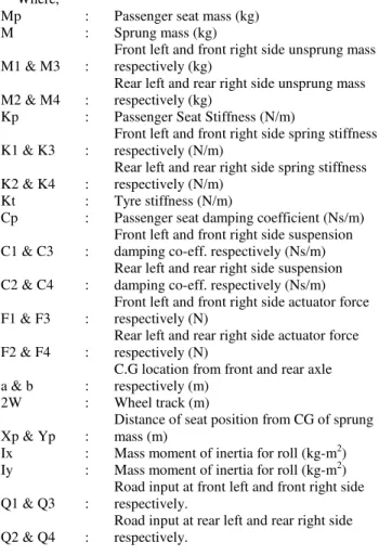
Where,
Mp : Passenger seat mass (kg)
M : Sprung mass (kg)
M1 & M3 :
Front left and front right side unsprung mass respectively (kg)
M2 & M4 :
Rear left and rear right side unsprung mass respectively (kg)
Kp : Passenger Seat Stiffness (N/m)
K1 & K3 :
Front left and front right side spring stiffness respectively (N/m)
K2 & K4 :
Rear left and rear right side spring stiffness respectively (N/m)
Kt : Tyre stiffness (N/m)
Cp : Passenger seat damping coefficient (Ns/m)
C1 & C3 :
Front left and front right side suspension damping co-eff. respectively (Ns/m)
C2 & C4 :
Rear left and rear right side suspension damping co-eff. respectively (Ns/m)
F1 & F3 :
Front left and front right side actuator force respectively (N)
F2 & F4 :
Rear left and rear right side actuator force respectively (N)
a & b :
C.G location from front and rear axle respectively (m)
2W : Wheel track (m)
Xp & Yp :
Distance of seat position from CG of sprung mass (m)
Ix : Mass moment of inertia for roll (kg-m2) Iy : Mass moment of inertia for roll (kg-m2)
Q1 & Q3 :
Road input at front left and front right side respectively.
Q2 & Q4 :
Road input at rear left and rear right side respectively.
A full car model with eight degrees of freedom is considered for analysis. Fig 1 shows a full car (8DOF) model consisting of passenger seat and sprung mass referring to the part of the car that is supported on springs and unsprung mass which refers to the mass of wheel assembly. The tire has been replaced with its equivalent stiffness and tire damping is neglected. The suspension, tire, passenger seat are modeled by linear springs in parallel with dampers. In the vehicle model sprung mass is considered to have 3DOF i.e. bounce, pitch and roll while passenger seat and four unsprung mass have 1DOF each.
Using the Newton’s second law of motion and free-body diagram concept, the following equations of motion are derived.
(
− − −)
+ ( − − − )=0+ • • • • • • φ θ φ
(
)
0 4 3 2 1 ) 4 ( 4 ) 4 ( 4 ) 3 ( 3 ) 3 ( 3 ) 2 ( 2 ) 2 ( 2 ) 1 ( 1 ) 1 ( 1 = − + − + − − − + − − − + − − + + − − + + − − − − − − − − − + + + − + + + − + − + − + − − • • • • • • • • • • • • • • • • • • • • • • bF aF bF aF Yp Xp Z Zp XpCp Yp Xp Z Zp XpKp Z W b Z bC Z W b Z bK Z W a Z aC Z W a Z aK Z W b Z bC Z W b Z bK Z W a Z aC Z W a Z aK Iy φ θ φ θ φ θ φ θ φ θ φ θ φ θ φ θ φ θ φ θ θ (4)(
1 1)
1 0 ) 1 ( 1 ) 1 ( 1 11 − − + − − − + − + − + =
• • • • • • F Q Z Kt Z W a Z C Z W a Z K Z
M θ φ θ φ (5)
(
2 2)
2 0) 2 ( 2 ) 2 ( 2 2
2Z••−K Z+b +W −Z −C Z•+b•+W•−Z• +KtZ −Q +F =
M θ φ θ φ (6)
(
3 3)
3 0) 3 ( 3 ) 3 ( 3 3
3Z••−K Z−a −W −Z −C Z•−a•−W•−Z• +KtZ −Q +F =
M θ φ θ φ (7)
(
4 4)
4 0) 4 ( 4 ) 4 ( 4 4
4Z••−K Z+b −W −Z −C Z•+b•−W•−Z• +KtZ −Q +F =
M θ φ θ φ (8)
Using following state space variables,
1
X
Zp= Zp• =X2 Z=X3 Z•=X4 φ=X5 φ•=X6
θ= X7 θ•=X8 Z1=X9 Z•1=X10 Z2=X11 Z•2=X12
13 3 X
Z = Z•3=X14 Z4=X15 Z•4=X16
Substituting above variables in Eq.(1-8) and writing the equations in state space representation form,
GF BQ AX
X= + +
• (9) Where, A16] A15 A14 A13 A12 A11 A10 A9 A8 A7 A6 A5 A4 A3 A2 1
[A T
A= 16] 15 14 13 12 11 10 9 8 7 6 5 4 3 2 1
[X X X X X X X X X X X X X X X X T
X= T B B B B B = 4 3 2 1 = 4 3 2 1 Q Q Q Q Q T G G G G G = 4 3 2 1 = 4 3 2 1 F F F F F
[
]
TB1= 0 0 0 0 0 0 0 0 0 (Kt/M1) 0 0 0 0 0 0
[
]
TB2= 0 0 0 0 0 0 0 0 0 0 0 (Kt/M2) 0 0 0 0
[
]
TB3=0 0 0 0 0 0 0 0 0 0 0 0 0 (Kt/M3) 0 0
[
]
TB4= 0 0 0 0 0 0 0 0 0 0 0 0 0 0 0 (Kt/M4)
T C4W K4W C3W K3W C2W -K2W -C1W -K1W -XpYpCp) -bWC4 -aC3W + bC2W + (-aC1W XpYpKp) -bWK4 -aK3W + bK2W + (-aK1W Cp) Yp -C4) + C3 + C2 + (C1 (W Kp) Yp -K4) + K3 + K2 + (K1 (W YpCp) + C4) -C3 -C2 + (W(C1 YpKp + K4) -K3 -K2 + (W(K1 CpYp KpY Ix 1 -= A6 2 2 2 2 T bC4 -bK4 -aC3 aK3 bC2 -bK2 -aC1 aK1 Cp) Xp -C4) + C3 + C2 + (C1 (a Kp) Xp -K4) + K3 + K2 + (K1 (a XpYpCp) -bWC4 -aC3W + bC2W + (-aC1W XpYpKp) -bWK4 -aK3W + bK2W + (-aK1W XpCp) -bC4 + aC3 -bC2 + (-aC1 XpKp) -bK4 + aK3 -bK2 + (-aK1 CpXp KpXp Iy 1 -= A8 2 2 2 2 T 0 0 0 0 0 0 C1 K1) + (Kt aC1 aK1 C1W K1W -C1 -K1 -0 0 M1 1 -= A10 T 0 0 0 0 C2 Kt) + (K2 0 0 bC2 -bK2 -C1W -K2W -C2 -K2 -0 0 M2 1 -= A12 T 0 0 C3 Kt) + (K3 0 0 0 0 aC3 aK3 C3W K3W C3 -K3 -0 0 M3 1 -= A14 T C4 Kt) + (K4 0 0 0 0 0 0 bC4 -bK4 -C4W K4W C4 -K4 -0 0 M4 1 -= A16
Active Suspension System
The linear time invariant system (LTI) is described by Eq.(9). For controller design it is assumed that all the states are available and also could be measured exactly. First of all let us consider a state variable feedback regulator (Ogata, 1996);
KX
F=− (10)
Where K is the state feedback gain matrix.
The optimization procedure consists of determining the control input F which minimizes the performance index. The performance index J represents the performance characteristic requirement as well as the controller input limitations. In this work LQR control scheme is used to find the control force required, for which one has evaluate the performance index J and hence design the optimal LQR controller. The optimization procedure consists of determining the control input F, which minimizes J, the performance characteristic requirement as well as the controller input limitations.
∫ ∞ + = 0 dt ) F R F X P X (
J T T (11)
Where 16] 15 14 13 12 11 10 9 8 7 6 5 4 3 2
1X X X X X X X X X X X X X X X T X [ X= also = 4 3 2 1 F F F F
F and P and R are positive and are called weighting
matrices.
The function inside the integral in Eq.(11) is a quadratic form and the matrices P and R are usually symmetric. It is assumed that R is positive definite and P is positive semi definite. If R is very large relative to P, which implies that the control energy is penalized heavily, the control effort will diminish at the expense of larger values for the state. When P is very large relative to R, which implies that the state is penalized heavily, the control effort rises to reduce the state, resulting in a damped system. P and R represent respective weights on different states and control channels respectively and are assumed accordingly.
Algebraic Riccati Equation. Linear optimal control theory provides the solution of Eq.(11) in terms of Eq.(10).
The gain matrix K is computed from;
E G R
K= −1 T (12)
Where the matrix E is evaluated being the solution of the Algebraic Riccati Equation ;
0
1 + =
−
+A E EGR−G E P
AE T T (13)
And substituting gain matrix K in eqn. 9 we get
BQ X GK A
X• =( − ) + (14)
While designing the LQR controller more weightage is given to ride comfort and an upper limit of 25N is kept to the controlling force depending on the design constraints to reduce cost function. Due to their effectiveness in searching optimal design parameters and obtaining globally optimal solution, the Genetic Algorithms are applied to find the optimal actuator configuration.
Passive Suspension System
For passive suspension system as there is no actuator force i.e. [F] =0 and Eq.(9) becomes
BQ AX
X• = + (15)
The Eq.(14) and Eq.(15) can be solved for frequency domain or time domain using Matlab [Ogata, 1996].
Optimization and Analysis
Analysis of the suspension system generally implies solving Eq.(1-8) for the time response of the system. The following optimization methods and procedure is adopted for analysis.
Optimization Problem Formualtion
The performance characteristics which are of most interest when designing the vehicle suspension are passenger ride comfort, road holding and suspension travel. The passenger ride comfort is related to passenger acceleration, suspension travel is related to relative distance between the unsprung mass and sprung mass and road handling is related to the tyre displacement.
Among the above three characteristics ride comfort is chosen to be the most important characteristic and is expressed in an objective function as
) t ( Zp RMS ) Z ( f
min = ••
As per ISO2631 standards the passenger feels highly comfortable if the weighted RMS acceleration is below 0.315 m/s2 (Wong, 1998, Griffin, 2003 and ISO: 2631-1-1997). So, it is considered as constraint.
0 315
0 2
1= f − . m/s ≤
g
At least 5 inches of suspension travel must be available in order to absorb a bump acceleration of one-half “g” without hitting the suspension stops and also an upper bound to maximum acceleration
should be kept so that at any time suspension will not hit suspension stops (Baumal et al., 1998 and Gillespie, 2003). Both these are taken as constraints
0 127 0 1
2=Z−Z − . m≤
g ,g3= Z−Z2−0.127m≤0
0 127 0 3
4=Z−Z − . m≤
g ,
0 127 0 4
5=Z−Z − . m≤
g , 6= −45 2≤0
• •
s / m . ) t ( Zp max g
Dynamic tyre force will increases with increase in tyre deflection so an upper bound to maximum tyre deflection is placed and it is considered as one more constraint (Baumal et al., 1998 and Gillespie, 2003).
0 0508 0 1 1
7=Z −Q − . m≤
g , g8= Z2−Q2−0.0508m≤0
0 0508 0 3 3
9= Z −Q − . m≤
g , g10=Z4−Q4−0.0508m≤0
The other performance characteristic viz. road holding is included as constraints and is restricted by (Baumal et al., 1998).
0 07 0 1
11=Z − . m≤
g , g12=Z2−0.07m≤0 0
07 0 3
13= Z − . m≤
g , g14=Z4−0.07m≤0
Human being feel comfortable within a frequency zone of 0.8 Hz and 1.5 Hz and also another criterion for good suspension system often considered is the maximum allowable jerk experienced by the passengers. Both these are added as two more constraints (Griffin, 2003 and Gillespie, 2003).
Hz . Wn .
g15=08≤ ≤15 , 16= −18 3≤0
• • •
s / m ) t ( Zp Max g
In order to make pitch motion die faster natural frequency of front suspension should be greater than the rear suspension and it is considered as constraint (Gillespie, 2003).
Wr Wf g17= >
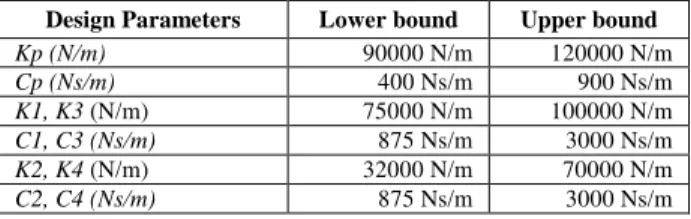
Table 1 (Panzade, 2005) gives the details of fixed parameters used in the analysis and the design variables are also restricted to ranges defined by the bounds as shown in table 2 (Panzade, 2005).
Table 1. Fixed parameters
Parameters Values Parameters Values
Kt 200000 N/m Iy 4140 kg-m2
Mp 100 kg 2W 1.450 m
M 2160 kg a 1.524 m
M1, M3 85 kg b 1.156 m M2, M4 60 kg Xp 0.234 m Ix 946 kg-m2 Yp 0.375 m
Table 2. Variable design parameter ranges,
Design Parameters Lower bound Upper bound
Kp (N/m) 90000 N/m 120000 N/m
Cp (Ns/m) 400 Ns/m 900 Ns/m
K1, K3 (N/m) 75000 N/m 100000 N/m
C1, C3 (Ns/m) 875 Ns/m 3000 Ns/m
K2, K4 (N/m) 32000 N/m 70000 N/m
Road Profile
A sinusoidal shape of the road profile as shown in Fig. 2 consisting of two successive depressions of depth h = 0.05 m, length λ = 20 m and vehicle velocity V = 20 m/s is used for analysis (Baumal et al., 1998).
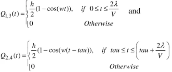
As a function of time, the road conditions are given by
≤ ≤ −
=
0
2 0 )), cos( 1 ( 2 ) ( 3 , 1
Otherwise V t if wt h
t Q
λ and
+ ≤ ≤ −
− =
0
2
)), ( cos( 1 ( 2 ) ( 4 , 2
Otherwise V tau t tau if tau t w h t Q
λ
Where tau and w are the time lag between front and rear wheels and the forcing frequency respectively and are given by
+
= V
b a
tau and
λ πV w= 2
In this study, the right and left sides have same amplitude road profile but there is a time delay of 0.2 sec and also the rear wheel will follows the same trajectory as the front wheels with a time delay of tau as shown in Fig.2. This road input will help to introduce bounce, pitch and roll motion simultaneously.
0 0.5 1 1.5 2 2.5 3 0
0.01 0.02 0.03 0.04 0.05 0.06
Time (sec) A
m plit u d e ( m
)
Front Left Rear Left Front Right Rear Right
Figure 2. Road profile.
Modified Objective Function
The constrained optimization problem is converted into unconstrained one using penalty approach. The modified objective function is stated as
c
G f
Y= + (16)
Where f is the initial objective function and Gc is a penalty when constraints are violated and is given as
∑
= ×
= 17
1 i
) , 0 max(
i
c g
G α (17)
In Eq.(17), ‘α’ is a penalty value which will vary between 8000 and 10000. A GA program is written in MatLAB, which initialize
suspension design variables. Then these values are passed into the 8DOF full car model to solve for the dynamic response of the system. These values are then substituted back into the GA process to calculate the fitness of the suspension design. This procedure is repeated until the stopping criterion is met.
Results and Discussions
This section is divided into two parts. The first gives the best parameters for the present models and comparison the results with simulated annealing method while the second part deals with simulation of present optimally designed suspensions.
The design results from the GA program for passive and active suspension are tabulated in table 3 In order to verify the validity of the results; the GA results were compared to those obtained by simulated annealing technique.
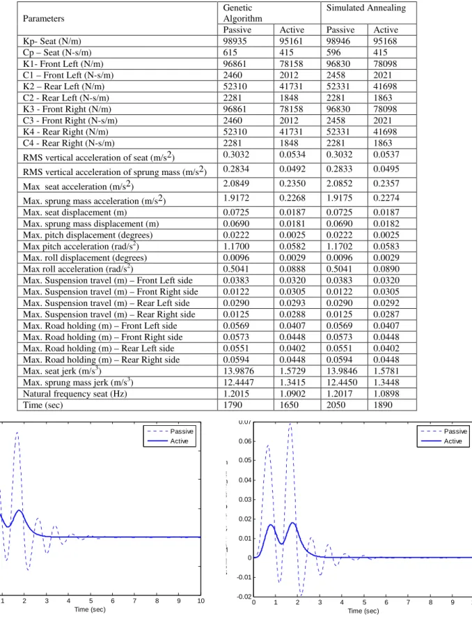
Simulation is performed using vehicle data illustrated in table 1, for road input defined in Fig. 2 and the optimal suspension parameters defined in table 3 using genetic algorithm. In table 3 it can seen the natural frequency of seat for both suspension systems are within the comfortable zone of 0.8-1.5 Hz, while passive suspension system the natural frequency is more compared to active since it use more stiffer suspension at front and rear.
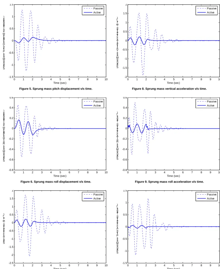
In Fig. 3 it can be observed that the reduction of the driver’s vertical displacement peak is approximately 74.2% in case of active suspension as compared with passive suspension and also settling time is reduced from 6 sec to 3.5 sec. Also it is observed that sprung mass vertical displacement is less in case of active suspension compare to passive suspension while pitch and roll displacement is amplified in active suspension and, consequently return to zero is also fast (Fig.4-6). This will occurs since during LQR controller design for active suspension more weightage is given to vertical displacement for comfortable ride.
From Fig. 7-8 it can be observed that seat acceleration and sprung mass vertical acceleration is reduced by 88.72% and 88.17% respectively in case of active suspension as compared with passive suspension and also settling time is reduced from 6.5 sec to 3 sec. Also the vertical weighted RMS acceleration of seat and sprung mass is reduced from 0.3032 m/s2 to 0.0534 m/s2 and 0.2834 m/s2 to 0.0492 m/s2 since in case of active LQR controller design more weightage is given ride comfort. It can also be observed sprung mass weighted RMS acceleration is less than seat since seat is located near front right side of tyre while for sprung mass weighted RMS acceleration is calculated at center of gravity of sprung mass.
From Fig. 9 it can be observed that range of the roll acceleration is 65% lower with active suspension than passive suspension. One should be remind here that this rolling motion is excited by time delay between the left and right side bump. Hence, the active suspension has proved to be definitely superior to the passive case.
With regards to pitch acceleration illustrated in Fig. 10, for active suspension the acceleration amplitude range is lower and consequently, returns to zero is very fast. In addition, disturbances of higher amplitude were recorded at about 0.6 sec and 1.6 sec. If we analyze the excitation in Fig. 2 one can observe that these disturbances are likely due to the phase angle of wheel motion slightly ahead of disturbance.
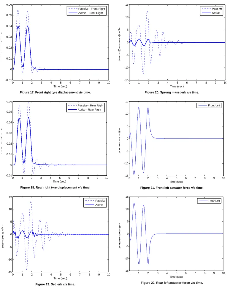
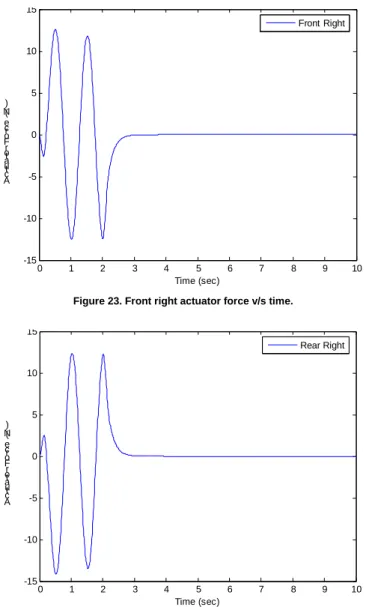
Also from Fig. 19 and 20 it can be observed that rate of change of acceleration is less in case of active suspension. Hence, jerk experienced by driver seat and sprung mass, for active suspension
jerk is very less compare to passive suspension. Figure 21-24 gives the actuator forces required for active suspension and all are well below the applied limits and practically implementable.
Table 3. Design results of genetic algorithm and simulated annealing method.
Genetic Algorithm
Simulated Annealing Parameters
Passive Active Passive Active
Kp- Seat (N/m) 98935 95161 98946 95168
Cp – Seat (N-s/m) 615 415 596 415
K1- Front Left (N/m) 96861 78158 96830 78098
C1 – Front Left (N-s/m) 2460 2012 2458 2021
K2 – Rear Left (N/m) 52310 41731 52331 41698
C2 - Rear Left (N-s/m) 2281 1848 2281 1863
K3 - Front Right (N/m) 96861 78158 96830 78098
C3 - Front Right (N-s/m) 2460 2012 2458 2021
K4 - Rear Right (N/m) 52310 41731 52331 41698
C4 - Rear Right (N-s/m) 2281 1848 2281 1863
RMS vertical acceleration of seat (m/s2) 0.3032 0.0534 0.3032 0.0537
RMS vertical acceleration of sprung mass (m/s2) 0.2834 0.0492 0.2833 0.0495
Max seat acceleration (m/s2) 2.0849 0.2350 2.0852 0.2357
Max. sprung mass acceleration (m/s2) 1.9172 0.2268 1.9175 0.2274
Max. seat displacement (m) 0.0725 0.0187 0.0725 0.0187
Max. sprung mass displacement (m) 0.0690 0.0181 0.0690 0.0182
Max. pitch displacement (degrees) 0.0222 0.0025 0.0222 0.0025
Max pitch acceleration (rad/s2) 1.1700 0.0582 1.1702 0.0583
Max. roll displacement (degrees) 0.0096 0.0029 0.0096 0.0029
Max roll acceleration (rad/s2) 0.5041 0.0888 0.5041 0.0890
Max. Suspension travel (m) – Front Left side 0.0383 0.0320 0.0383 0.0320 Max. Suspension travel (m) – Front Right side 0.0122 0.0305 0.0122 0.0305 Max. Suspension travel (m) – Rear Left side 0.0290 0.0293 0.0290 0.0292 Max. Suspension travel (m) – Rear Right side 0.0125 0.0288 0.0125 0.0287 Max. Road holding (m) – Front Left side 0.0569 0.0407 0.0569 0.0407 Max. Road holding (m) – Front Right side 0.0573 0.0448 0.0573 0.0448
Max. Road holding (m) – Rear Left side 0.0551 0.0402 0.0551 0.0402
Max. Road holding (m) – Rear Right side 0.0594 0.0448 0.0594 0.0448
Max. seat jerk (m/s3) 13.9876 1.5729 13.9846 1.5781
Max. sprung mass jerk (m/s3) 12.4447 1.3415 12.4450 1.3448
Natural frequency seat (Hz) 1.2015 1.0902 1.2017 1.0898
Time (sec) 1790 1650 2050 1890
0 1 2 3 4 5 6 7 8 9 10 -0.04
-0.02 0 0.02 0.04 0.06 0.08
Time (sec) S
e at Dis pl ac e me nt ( m
)
Passive Active
Figure 3. Seat displacement v/s time.
0 1 2 3 4 5 6 7 8 9 10 -0.02
-0.01 0 0.01 0.02 0.03 0.04 0.05 0.06 0.07
Time (sec) Spr
u n g Ma s s Ve rtic al Dis pl a c e me nt ( m
)
Passive Active
0 1 2 3 4 5 6 7 8 9 10 -1.5
-1 -0.5 0 0.5 1 1.5
Time (sec) Spr
u n g Ma s s Pit c h Dis pl a c e me nt (d e gr e e)
Passive Active
Figure 5. Sprung mass pitch displacement v/s time.
0 1 2 3 4 5 6 7 8 9 10 -0.8
-0.6 -0.4 -0.2 0 0.2 0.4 0.6
Time (sec) Spr
u n g Ma s s Ro ll Dis pl a c e me nt (d e gr e e)
Passive Active
Figure 6. Sprung mass roll displacement v/s time.
0 1 2 3 4 5 6 7 8 9 10 -2.5
-2 -1.5 -1 -0.5 0 0.5 1 1.5 2
Time (sec) Se
at Ac cle ra ti o n ( m/s 2)
Passive Active
Figure 7. Seat acceleration v/s time.
0 1 2 3 4 5 6 7 8 9 10 -2
-1.5 -1 -0.5 0 0.5 1 1.5 2
Time (sec) Spr
u n g Ma s s Ve rtic al Ac cle ra ti o n ( m/s 2)
Passive Active
Figure 8. Sprung mass vertical acceleration v/s time.
0 1 2 3 4 5 6 7 8 9 10 -0.8
-0.6 -0.4 -0.2 0 0.2 0.4 0.6
Time (sec) Spr
u n g Ma s s Ro ll Ac cle ra ti o n (ra d/s 2)
Passive Active
Figure 9. Sprung mass roll acceleration v/s time.
0 1 2 3 4 5 6 7 8 9 10 -1.5
-1 -0.5 0 0.5 1 1.5
Time (sec) Spr
u n g Ma s s Pit c h Ac cle ra ti o n (ra d/s 2)
Passive Active
0 1 2 3 4 5 6 7 8 9 10 -0.04
-0.03 -0.02 -0.01 0 0.01 0.02 0.03 0.04
Time (sec) Su
s p e n sio n T ra v el ( m )
Passive - Front Left Active - Front Left
Figure 11. Front left suspension travel v/s time.
0 1 2 3 4 5 6 7 8 9 10 -0.035
-0.03 -0.025 -0.02 -0.015 -0.01 -0.005 0 0.005 0.01 0.015
Time (sec) S
u s p e n sio n T ra v el ( m
)
Passive - Rear Left Active - Rear Left
Figure 12. Rear left suspension travel v/s time.
0 1 2 3 4 5 6 7 8 9 10 -0.03
-0.02 -0.01 0 0.01 0.02 0.03
Time (sec) Su
s p e n sio n T ra v el ( m )
Passive - Front Right Active - Front Right
Figure 13. Front right suspension travel v/s time.
0 1 2 3 4 5 6 7 8 9 10 -0.03
-0.025 -0.02 -0.015 -0.01 -0.005 0 0.005 0.01 0.015
Time (sec) Su
s p e n sio n T ra v el ( m )
Passive - Rear Right Active - Rear Right
Figure 14. Rear right suspension travel v/s time.
0 1 2 3 4 5 6 7 8 9 10 -0.01
0 0.01 0.02 0.03 0.04 0.05 0.06
Time (sec) T
yr e Dis pl a c e me nt ( m
)
Passive - Front Left Active - Front Left
Figure 15. Front left tyre displacement v/s time.
0 1 2 3 4 5 6 7 8 9 10 -0.01
0 0.01 0.02 0.03 0.04 0.05 0.06
Time (sec) Tyr
e Dis pl a c e me nt ( m )
Passive - Rear Left Active - Rear Left
0 1 2 3 4 5 6 7 8 9 10 -0.01
0 0.01 0.02 0.03 0.04 0.05 0.06
Time (sec) Tyr
e Dis pl ac e me nt ( m
)
Passive - Front Right Active - Front Right
Figure 17. Front right tyre displacement v/s time.
0 1 2 3 4 5 6 7 8 9 10 -0.01
0 0.01 0.02 0.03 0.04 0.05 0.06
Time (sec) Tyr
e Dis pl ac e me nt ( m
)
Passive - Rear Right Active - Rear Right
Figure 18. Rear right tyre displacement v/s time.
0 1 2 3 4 5 6 7 8 9 10 -15
-10 -5 0 5 10 15
Time (sec) S
e at J erk ( m/s 3)
Passive Active
Figure 19. Set jerk v/s time.
0 1 2 3 4 5 6 7 8 9 10 -15
-10 -5 0 5 10 15
Time (sec) Spr
u n g Ma s s J erk ( m/s 3)
Passive Active
Figure 20. Sprung mass jerk v/s time.
0 1 2 3 4 5 6 7 8 9 10 -15
-10 -5 0 5 10 15
Time (sec) A
ctu ato r F orc e ( N)
Front Left
Figure 21. Front left actuator force v/s time.
0 1 2 3 4 5 6 7 8 9 10 -15
-10 -5 0 5 10 15
Time (sec) Ac
tu ato r Fo rc e ( N)
Rear Left
0 1 2 3 4 5 6 7 8 9 10 -15
-10 -5 0 5 10 15
Time (sec) Ac
tu ato r Fo rc e ( N)
Front Right
Figure 23. Front right actuator force v/s time.
0 1 2 3 4 5 6 7 8 9 10 -15
-10 -5 0 5 10 15
Time (sec) Ac
tu ato r F orc e ( N)
Rear Right
Figure 24. Rear right actuator force v/s time.
Conclusion
Considering the power and capabilities of GA, the present work has attempted to design optimal vehicle suspensions using it. Design objectives such as maximum bouncing acceleration of seat and sprung mass, root mean square (RMS) weighted acceleration of seat and sprung mass as per ISO2631 standards, jerk, suspension travel, road holding and tyre deflection are introduced for accessing comfortability of the suspension. While the searching space of the parameters is very large, the solution space is very tight due to the presence of various constraints. Therefore, the constrained optimization problem is converted into unconstrained one using penalty function approach.
In order to verify the validity of the results, the GA results were compared to those obtained by simulated annealing technique and found to yields similar performance measures. This validates the GA results and also demonstrates that there exists other feasible design, which is able to achieve the same objective.
From the simulation results, it can be observed that the reduction of the driver’s vertical displacement peak is approximately 74.2% in case of active suspension as compared with passive suspension and
also settling time is reduced from 6 sec to 3.5 sec. Also the vertical weighted RMS acceleration of seat and sprung mass is reduced from 0.3032 m/s2 to 0.0534 m/s2 and 0.2834 m/s2 to 0.0492 m/s2 using active LQR controller design since more weightage is given ride comfort. In case of active suspension travel increases by 56-60% than passive suspension to provide more ride comfort i.e. less displacement of sprung mass while tyre displacement is reduced by 28.5% to give better road holding, indicating active suspension system has better potential to improve both comfort and road holding.
References
Ahmadian, M.T., Sedeh, R.S., and Abdollahpour, R., “Application of Car Active Suspension in Vertical Acceleration Reduction of Vehicle Due to Road Excitation and Its Effect on Human Health”, International Journal of Scientific Research (In press).
Alkhatib, R., Jazar, G.N., and Golnaraghi, M.F., 2004, “Optimal Design of Passive Linear Suspension Using Genetic Algorithm”, Journal of Sound and Vibration, Vol. 275, pp. 665-691.
Baumal, A.E., McPhee, J.J., and Calamai, P.H., 1998, “Application of Genetic Algorithms to the Design Optimization of an Active Vehicle Suspension System”, Computer Methods in Applied Mechanics and Engineering, Vol. 163, pp. 87-94.
Bourmistrova A, Storey I and Subic A, 2005, “Multiobjective Optimisation of Active and Semi-Active Suspension Systems with Application of Evolutionary Algorithm”, International Conference on Modeling and Simulation, Melbourne, 12-15 December 2005.
Gao Huijun, Lam James and Wang Changhong, 2006, “Multi-Objective Control of Vehicle Active Suspension Systems via Load-Dependent Controllers”, Journal of Sound and Vibration, Vol. 290, pp. 654-675.
Gillespie Thomas D., 2003, “Fundamentals of Vehicle Dynamics”, Society of Automotive Engineers, Warrendale.
Gobbi, M. and Mastinu, G., 2001, “Analytical Description and Optimization of the Dynamic Behaviour of Passively Suspended Road Vehicles”, Journal of Sound and Vibration, Vol. 245, No. 3, pp. 457-481.
Griffin, M.J., 2003, “Handbook of human vibration”, Academic press, New York.
Hemiter Marc E., 2001, “Programming in Matlab”, Thomson Learning, Singapore.
ISO: 2631-1, 1997, “Mechanical vibration and shock - Evaluation of human exposure to whole-body vibration”.
Mantaras Daniel A., and Luque Pablo, 2006, “Ride Comfort Performance of Different Active Suspension Systems”, International Journal of Vehicle Design, Vol. 40, No. 1/2/3, pp. 106-125.
Ogata, K., 1996, “Modern Control Engineering”, Prentice-Hall, New Delhi, 3rd edition.
Panzade, P.K., 2005, “Modeling and Analysis of full vehicle for ride and handling”, M.E. Thesis, PSG College of Technology, Coimbatore.
Rettig Uwe, and Stryk Oskar von, 2005, “Optimal and Robust Damping Control for Semi-Active Vehicle Suspension”, Proc. ENOC-2005, Eindhoven, Netherlands, 7-12 August 2005.
Rill, Georg. 2006, “Vehicle modeling by subsystems”, J. Braz. Soc. Mech. Sci.& Eng., Vol.28, no.4, p.430-442.
Roumy Jean Gabriel, Boulet Benoit, and Dionne Dany, 2004, “Active Control of Vibrations Transmitted Through a Car Suspension”, International Journal of Vehicle Autonomous Systems, Vol. 2, No.3/4, pp. 236-254.
Sharkawy, A.B., 2005, “Fuzzy and Adaptive Fuzzy Control for the Automobiles’ Active Suspension System”, Vehicle System Dynamics, Vol. 43, No. 11, pp. 795-806.
Sun Lu, 2002, “Optimum Design of Road-Friendly Vehicle Suspension Systems Subjected to Rough Pavement Surfaces”, Journal of Applied Mathematical Modelling, Vol. 26, pp. 635-652.
Wong, J.Y., 1998, “Theory of Ground Vehicles”, John Wiley and Sons Inc., New York.