Jay Pal Singh
[email protected] Advanced Institute of Tech. & Management Depart. of Humanities & Applied Sciences 121105 Palwal, Haryana, IndiaNaseem Ahmad
[email protected]Jamia Millia Islamia Department of Mathematics 110 025 New Delhi, India
Analysis of a Porous-Inclined Slider
Bearing Lubricated with Magnetic
Fluid Considering Thermal Effects
with Slip Velocity
A theoretical model of a porous-inclined slider bearing lubricated with magnetic fluid has been considered together with slip velocity boundary condition. Our aim is to study the influence of various dimensionless parameters arising out of the analysis of the model. By assuming the viscosity µ =µ0exp
[
−β(
tm −t0)
]
of magnetic fluid, the expressions for mean temperature and load capacity have been obtained. It has been observed that both mean temperature field and load capacity are the functions of slip parameter, magnetic parameter, thermal parameter and permeability parameter. The dependence of the mean temperature field as well as of load capacity on these parameters has been seen graphically.Keywords: magnetic fluid, slip velocity, porous inclined-slider bearing, thermal effects, load capacity
Introduction1
The lubrication behavior of different Newtonian and non-Newtonian fluids has been examined and analyzed by many researchers recently. It has been noted that the use of non-Newtonian fluids as lubricants becomes more important than the use of Newtonian fluids. It is a well-reported fact that the lubricants with stable suspensions of fine particles of insoluble solids having different material characteristics can be used as the viscosity index improver so that the viscosity variation with temperature may be prevented. It has been revealed that the behavior of such fluid is not Newtonian but non-Newtonian (Pal et al., 2002). For understanding frictional behavior and also for defining the physical conditions met by the oil in its passage through the conjunction of the disks, the knowledge of the temperature in the lubricant film is required. Due to the shearing of the oil in the film, the frictional heat exists (Crook, 1961). Because of the strong dependence of the viscosity on temperature, the temperature generated inside the film by the frictional heating causes an effective change in lubricant viscosity. Consequently, the viscosity must be assumed to be a function of temperature (Rodkiewicz and Dayson, 1974). Furthermore, in a heavily loaded system under hydrodynamic or EHD conditions, where high pressure exceeding 107
dyne cm−2 is encountered, the
lubricant viscosity is no longer insensitive to the pressure. Crook (1963) observed a 1000-fold increase in the viscosity ratio on raising the load from 2.5 × 10⁷ to 19.7 × 10⁷ dyne
cm−1. Archard et
al. (1961) and Dowson and Whitaker (1965), among the pioneers in this field, also emphasized the need to consider the variation in viscosity with pressure. It is therefore necessary to consider the effect of pressure and temperature on the lubricant viscosity (Cheng and Sternlicht, 1965; Kannel andWalowit, 1971; Rohde and Ezzat, 1974). In addition, the classical theory of hydrodynamic lubrication implicitly assumes that the lubricant behaves, essentially, as a Newtonian viscous fluid. This assumption, however, is not valid for fluids such as molten plastics, pulps, slurries, emulsions, greases, etc. These fluids exhibit non-Newtonian behavior and are widely used as lubricant in various lubrication flows. Therefore, the non-Newtonian behavior of the fluid in lubrication is also of considerable interest (Prasad et al., 1987).
The use of magnetic fluids has led to the development of many new energy devices and instruments. Magnetically cooled
Paper received 16 July 2010. Paper accepted 30 March 2011. Technical Editor: Monica Naccache
high-fidelity speakers, computer disc drives and semiconductors are already commercially available. Magnetic fluids are prepared by suspending ferromagnetic grains in magnetic non-conducting liquids such as dieters, kerosene, hydrocarbons and fluorocarbons. Ferromagnetic fluids, the non-conducting colloidal suspension of solid magnetic particles of sub-domain size in carrier liquids, are responsible for the development of several mechanical and electronic devices based on them (Ram and Verma, 1999). A typical magnetic fluid is prepared by suspending Fe3O4 particles of size 100 Å which are coated with oleic acid in
a diester. The most important property of magnetic fluids is that they can be made to adhere to any desired surface with the aid of magnets. When a magnetic field is applied, each particle experiences a force which causes it to move. When all the particles start moving, they cause the colloidal homogeneous suspension to move en masse (Agrawal, 1986).
Ochonski (2007) considered sliding bearings lubricated with magnetic fluids and suggested a new design of magnetic fluid-based sliding bearings. Patel (1980) studied the effect of slip velocity on the behavior of a squeeze film between two circular disks, the upper disk having a porous facing backed by solid housing, in the presence of a uniform transverse magnetic field. These investigations show that the effect of slip velocity reduces the load capacity of the bearing. Patel andGupta (1983) used this slip condition at a porous boundary for hydrodynamic lubrication to analyze the problem of an inclined porous slider bearing. They suggested that minimization of the slip parameter is essential to increase the load capacity. Sinha et al. (2001) studied thermal effects in externally pressurized porous conical bearings with variable viscosity. Ahmad and Singh (2007a) used slip condition at a porous boundary for an inclined slider bearing without thermal effect. Further, Ahmad and Singh (2004b) investigated an inclined slider bearing with thermal effect.
Nomenclature
a
= inlet-outlet ratio0
B = non-dimensional coefficient of temperature
p
c
= specific heatE
= Eckert numberh
= dimensional film heightH
r
= external magnetic field
h
= non-dimensional film height 0h
= minimum film thickness 1h
= maximum film thicknessk
= porosity of the porous matrixk
= thermal conductivityl
= bearing wall thicknessL
= bearing width Mr
= magnetization vector
∗
M
= co-rotational derivative of M rM
= magnitude of the magnetization vectorM
= non-dimensional coefficient of viscosity p = fluid pressureP = non-dimensional fluid pressure
r
P = Prandtl number
s
1
= non-dimensional slip parameter s =α k12, slip parametert
= temperature of the fluid 0t
= temperature at p = 0 (i.e., ambient pressure)m
t
= mean temperature across the film thickness mT
= non-dimensional mean temperatureT = non-dimensional temperature field u = velocity component along the x-axis
U = uniform sliding velocity component along the x-axis
0
u
= non-dimensional velocity component along the x-axisV
r
= fluid velocity
W = non-dimensional load capacity x, y = Cartesian coordinates
x
= non-dimensional x-coordinateα
= slip coefficient∗
α
= material constantβ
= coefficient of temperatureβ
= permeability parameterµ
= coefficient of viscosity 0µ
= free space permeability ∗µ
= non-dimensional magnetic parameterµ
= magnetic susceptibilityFormulation of the Problem
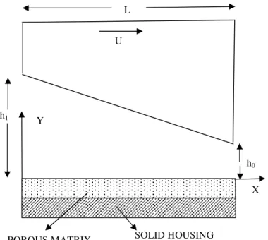
The configuration of a porous-inclined slider bearing lubricated with an incompressible magnetic fluid is shown in Fig. 1.
Figure 1. A porous-inclined slider bearing lubricated with magnetic fluid.
According to Agrawal (1986), the equations governing the flow of incompressible magnetic fluid in D=
{
( )
x,y :0≤x≤L,0≤y≤h}
are as follows:
( )
( )
× × ∇ + ∇ ⋅ + ∇ + ∇ − =
∇ ⋅ + ∂
∂ ∗ ∗
M M M H
M V p V V t V
r r r r r r r r r r r r
2
0
2 µ ρα
µ
ρ
(1)
0 V = ⋅ ∇r r
(2)
where
V
,
p
r
, ρ,
µ
,α
∗,M
r
, M, M*, H r
and
µ
0 are the fluid velocity, the pressure, the density, the coefficient of viscosity, a material constant, the magnetization vector, the magnitude of the magnetization vector, the co-rotational derivative of Mr , the external magnetic field and the free-space permeability, respectively.
Because of magnetic fluid, we have the following relations based on Maxwell’s equations:
φ ∇ − = =
×
∇r r r r
H ,
0
H (3)
(
H M)
BB
r r r r
r
+ = =
⋅
∇ 0, µ0 (4)
H M
r r
µ
= (5)
where
µ
is the magnetic susceptibility.The equation of continuity in the porous region is given by
0 = ∂ ∂ + ∂ ∂
y v x
u (6)
Under the normal conditions of lubrication theory and neglecting the self-field due to magnetization, we get the simplified forms of Eqs. (1) through (5) as:
SOLID HOUSING U
h1 Y
L
h0
X
0 2 2 0 2 2 = − ∂ ∂ − ∂ ∂ H p x y
u µ µ
µ (7) 0 = ∂ ∂ + ∂ ∂ y v x
u (8)
0 2
2
0 =
− ∂
∂ p H
y
µ
µ
(9) − ∂ ∂ −
= 0 2
2 H
p x k
u
µ
µ
µ
(10) − ∂ ∂ −
= 0 2
2 H
p y k
v µ µ
µ (11)
Substituting Eqs. (10) and (11) into Eq. (6), one obtains
0 2 2 2 0 2 2 2 0 2 2 = − ∂ ∂ + − ∂ ∂ H p y H p x µ µ µ
µ (12)
The relevant boundary condition for the velocity field in the lubricant region is
h y at U
u = = (13)
where
U
is the uniform sliding velocity component along the x-axisand h is the dimensional film height.
As the slip velocity at the porous matrix is being introduced, the slip velocity due to Patel and Gupta (1983) is given by
1 2 0 α ∂ = = ∂ u
u at y y
k
(14)
where k is the porosity of the porous matrix and a is the slip
coefficient which depends on the structure of the porous material. For pressure, the appropriate boundary conditions are
L x at
p=0 =0, (15)
where Lis the width of the bearing.
Solving Eq. (7) and applying the boundary conditions (13) and (14), we have the velocity component as
(
)
(
sy)
sh H p x h U H p x y u − − − ∂ ∂ − + − ∂ ∂ = 1 1 2 2 2 2 2 0 2 2 0 2 µ µ µ µ µ µ (16) where 2 1 k
s= α is the slip parameter.
Using Eqs. (8), (12) and (15), one can get the Reynolds equation in the following form:
{
}
(
kl klsh h h s)
sh A sh Uh H px 3 4
2 0 4 12 12 ) 1 ( 12 ) 2 ( 6
2 − + −
− − − = − ∂
∂ µ µ µ (17)
where A is the constant of integration and
l
is the bearing wallthickness.
Heat Transfer Problem
We assume that the flow of lubricant is thermally active while surfaces are not. Under these assumptions, the energy equation is simplified to get
2 2 2 ∂ ∂ − = ∂ ∂ y u y t
k µ (18)
Let the viscosity µ be variable and it varies with temperature raised by frictional heat generated by flow of fluid having thermal conductivity k .Theexpression µ due to Prasad et al. (1987) is
(
)
[
0]
0exp − tm −t
=µ β
µ (19)
where
µ
0 and t0 are, respectively, the viscosity coefficient and temperature when p = 0 (ambient pressure).β
is the thermalcoefficient and tm is the mean temperature across the film
thickness
h
, which is defined as(
)
∫
= h
m h tdy
t
0
1 (20)
The boundary conditions for the temperature field in the lubricant region are
0 0
t=t at y= and y= h (21)
Introducing the following dimensionless variables:
0 0 0 0
2
3 0
0 3
0 0 0
2
2 *
0 0 0
0 0 0
0 12 , , , , 12 , , , , , , , , m m p r p
x y h A
x y h M A
L h h Uh
ph t
u t kl
u P T T
U UL t t h
c U h L
P E B t s sh
k c t U
µ µ
β µ
µ β µ µ µ
µ
= = = = =
= = = = =
= = = = =
where
c
p, h , h0, h1 and β are the specific heat, thenon-dimensional film height, the minimum film thickness, the
maximum film thickness and the permeability parameter, respectively.
The non-dimensional forms of Eqs. (16), (18), (19) and (20) are
(
)
(
) (
)
(
)
2 2
0
1
1 1 1
2 2 2 2 1
s y
y h
u P x x P x x
x x s h
µ∗ µ∗ −
∂ ∂ = − − + − − − ∂ ∂ − (22) 2 0 2 2 . ∂ ∂ − = ∂ ∂ y u E P M y T r (23)
(
)
{
B T 1}
exp
( )
h
T
d
y
T
m=
1
∫
0h(25)
where P,
µ
∗, 1 s, M , Pr, E,B0, Tm and Pr.E are, respectively, the non-dimensional fluid pressure, magnetic parameter, slip parameter, coefficient of viscosity, Prandtl number, Eckert number, coefficient of temperature, mean temperature and thermal parameter.Using Eqs. (22), (23) and boundary conditions T = 1 at
y
=
0
and at
y
=
h
, we obtain the temperature field(
)
(
)
(
)
(
)
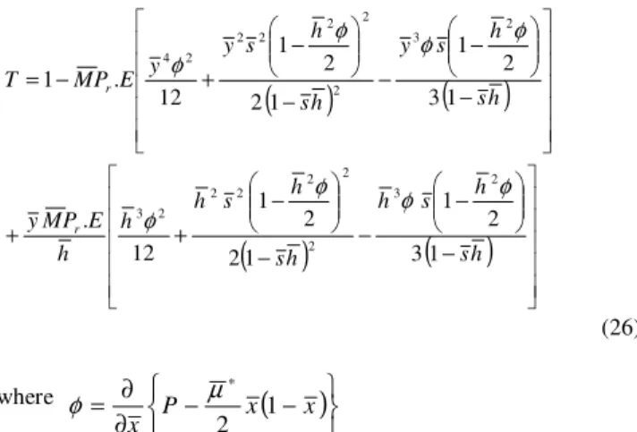
− − − − − + + − − − − − + − = h s h s h h s h s h h h E P M y h s h s y h s h s y y E P M T r r 1 3 2 1 1 2 2 1 12 . 1 3 2 1 1 2 2 1 12 . 1 2 3 2 2 2 2 2 2 3 2 3 2 2 2 2 2 2 4 φ φ φ φ φ φ φ φ (26)where
(
)
− − ∂ ∂
= P ∗ x x
x 2 1
µ
φ
Putting this value of T into Eq. (25) and on simplifying, we
obtain mean temperature as
(
)
( )
( )
(
)
− − − − − + + + = h s h s h h s h h s h h E P M T r m 1 2 5 1 4 5 6 240 . 1 2 3 2 2 2 4 2 24
φ
φ
φ
φ
φ
(27)
The dimensionless form of Eq. (17) is
(
)
(
)
(
) (
)
+ − + − + − = − − ∂ ∂ ∗ 3 3 3 3 4 1 6 ) 12 ( 1 2 2 1 h h h s h A h A h s x x P β β µ (28)where the film thickness h(x) of the inclined slider bearing is
given by h(x)=a−
(
a−1)
x, where a =h1 h0, 0≤ x≤1 . In particular, we take the inlet-outlet ratiox x h h h
a= 1 0=2⇒ ( )=2− = 2
To compute load capacity, we use the formula
∫
∫
= −= 01 01 dx
x d dP x x d P W (29) Now, using Eqs. (27) and (29), we obtain load capacity of the
bearing as
(
)
( )( )( )
(
) (
)
(
) (
)
(
)
x d h s h s h h h s h A h A h s s E P h h s T e s h s h s h h x W r m Tm∫
+ + − + − + − − − − − + − + − = − ∗ 1 0 2 2 3 3 3 3 2 2 2 1 7 . 0 3 2 2 3 10 10 4 1 6 12 1 20 . 1 1 240 5 12 6 6 1 12 β β µ (30)Discussion and Results
On the basis of the analysis and computation carried out for this problem, we recommended the following findings:
1. Figure 2 is a graph of mean temperature versus permeability parameter. It is seen that the mean temperature of the bearing increases as the permeability parameter increases. It has been noticed that mean temperature is increasing exponentially for
β
〉0.1.052 1.054 1.056 1.058 1.06 1.062 1.064
0 0.2 0.4 0.6 β 0.8 1 1.2 1.4
Tm
Figure 2. Mean temperature vs. permeability parameter at 1s=3,Pr.E=1.2,x=0.6.
2. Figure 3 shows a graph of mean temperature versus slip parameter. As the slip parameter increases, the mean temperature decreases. Physically, introduction of slip velocity reduces frictional between fluid and boundary due to which production heat may be reduced. This results in a fall in temperature.
1 1.05 1.1 1.15 1.2 1.25 1.3 1.35 1.4
2 2.5 1/s 3 3.5 4
Tm
Figure 3. Mean temperature vs. slip parameter at β=1.3,Pr.E=1.2,x=0.6.
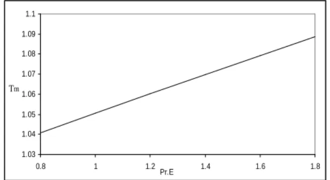
1.03 1.04 1.05 1.06 1.07 1.08 1.09 1.1
0.8 1 1.2 1.4 1.6 1.8
Pr.E
Tm
Figure 4. Mean temperature vs. thermal parameter at 1s=3,β=1.3,x=0.6.
4. Figure 5 clarifies the behavior of mean temperature against magnetic parameter. According to this graph, mean temperature increases with the increase of the magnetic parameter. The figure shows that Tm is the linear function of
µ
.2.3 2.35 2.4 2.45 2.5 2.55 2.6
12 14 16 18 20 22
Tm
µ*
_
Figure 5. Mean temperature vs. magnetic parameter at 1s=3,P.E=1.2,x=0.6
r .
5. In Fig. 6, the slip parameter and the thermal parameter have been fixed and a graph of load capacity versus permeability parameter has been drawn to read the influence of the magnetic parameter. According to this graph, the impact of the permeability parameter is almost nil. It has also been noted that as the magnetic parameter increases, the load capacity also increases. This trend of dependence of load capacity on the magnetic parameter is also supported by the researches done by Agrawal (1986) and Ahmad and Singh (2007a).
0.6 0.7 0.8 0.9 1 1.1 1.2 1.3 1.4 1.5 1.6
0 0.2 0.4 0.6 0.8 1 1.2 1.4
W
β µ = 14 µ = 16 µ = 18 µ = 20
µ = 12 * _
* * *
*
Figure 6. Load capacity vs. permeability parameter for different values of the magnetic parameter at 1s=3,P.E=1.2
r .
6. In Fig. 7, a graph of load capacity versus slip parameter has been plotted for different values of the magnetic parameter, while the permeability and thermal parameters are taken as constant. It is seen that the influence of the slip parameter is not remarkable, but the magnetic parameter boosts the load capacity.
0.6 0.7 0.8 0.9 1 1.1 1.2 1.3 1.4 1.5 1.6
2.5 2.75 3 3.25 3.5 3.75 4
W
µ = 18
µ = 16
µ = 14
µ = 12 µ = 20
1/s * * * * *
Figure 7. Load capacity vs. slip parameter for different values of the magnetic parameter at P.E=1.2,β =1.3
r .
7. Figure 8 exhibits the variation of the load capacity with respect to the thermal parameter as well as the magnetic parameter. It is concluded that the load capacity decreases slightly when the thermal parameter increases from 0.8 to 1.0, and then it is almost constant beyond that. Therefore, the load capacity of the bearing is optimized when the thermal parameter is 0.8.
0.6 0.7 0.8 0.9 1 1.1 1.2 1.3 1.4 1.5 1.6
0.8 1 1.2 1.4 1.6 1.8
W
µ = 18 µ = 20
µ = 16
µ = 14
µ = 12
Pr.E *
*
*
*
*
Figure 8. Load capacity vs. thermal parameter for different values of the magnetic parameter at 1s=3,β=1.3.
Conclusions
A theoretical model of lubrication theory has been analyzed where magnetic fluid has been considered as lubricant with slip velocity effects. It has been recommended that permeability of the porous matrix accelerates mean temperature while slip velocity decelerates it. It has been concluded that mean temperature increases linearly with the thermal parameter.
The load capacity W has been studied in respect of the slip
on load capacity W while the thermal parameter Pr.E has an influence within 0.8〈Pr.E〈1.0 only.
The magnetic parameter boosts the load capacity Wof the slider
bearing.
Acknowledgement
The authors are thankful to Mr. Shivhari Dikshit, Assistant Professor in English, AITM, Palwal, who helped in improving the English language of this paper.
References
Agrawal, V.K., 1986, “Magnetic-fluid based porous inclined slider bearing”, Wear, Vol. 107, pp. 133-139.
Ahmad, N. and Singh, J.P., 2007a, “Analysis of a porous inclined slider bearing lubricated with a magnetic fluid considering slip velocity”, Proc. IMechE Part N: J. Nanoengineering and Nanosystems, Vol. 221(N3), pp. 81-85.
Ahmad, N. and Singh, J.P., 2004b, “Magnetic fluid based porous inclined slider bearing considering thermal effects”, Proc. 2nd BSME-ASME International Conference on Thermal Engineering, Vol. II, pp. 1019-1025.
Archard, G.D., Gair, E.C., and Hirst, W., 1961, “The EHD lubrication of rollers”, Proc. Roy. Soc. London, Ser. A262, 51, pp. 51-65.
Cheng, H.S., and Sternlicht, B., 1965, “A numerical solution for the pressure, temperature and film thickness between two infinitely long lubricated rolling and sliding cylinders under heavy load”, ASME Trans., Ser. D., 87(3), pp. 695-707.
Crook, A.W., 1961, “The lubrication of rollers -III. A theoretical discussion of friction and the temperature in the oil films”, Philos. Trans. Roy. Soc. London, Ser. A, Vol. 254, pp. 237-258.
Crook, A.W., 1963, “The lubrication of rollers IV. Measurement of friction and effective viscosity”, Philos. Trans. R. Soc. London, Ser. A, Vol. 255, pp. 281-312.
Dowson, D., and Whitaker, A.V., 1965, “The isothermal lubrication of cylinders”, ASLE Trans., Vol. 8, pp. 224-234.
Hughes, W.F. and Yong, F.J., 1966, “The Electromagnetodynamics of fluid”, 45 p.
Kannel, J.W., and Walowit, J.A., 1971, “Simplified analysis for traction between rolling sliding EHD contacts”, J. Lubr. Technol., Vol.93, pp. 39-46. Pal, A.K., Das, N.C., and Chaudhary, R., 2002, “A Study of load capacity of finite slider bearings lubricated with couple stress fluids considering thermal effects”, Indian J. Pure and Appl. Maths, 33(10), pp. 1529-1540.
Patel, K.C. and Gupta, J.L., 1983, “Hydrodynamic lubrication of a porous slider bearing with slip velocity”, Wear, Vol. 85, pp. 309-317.
Patel, K.C., 1980, “The hydro magnetic squeeze film between porous circular disks with velocity slip”, Wear, Vol. 58(2), pp. 275-281.
Prasad, D., Singh, P., and Sinha, P., 1987, “Thermal and squeezing effects in non-Newtonian fluid film lubrication of rollers”, Wear, Vol. 119, pp. 175-190.
Ram, P. and Verma, P.D.S., 1999, “Ferro fluid lubrication in porous inclined slider bearing”, Indian J. Pure and Appl. Maths,Vol. 30(12), pp. 1273-1281.
Rodkiewicz, C.M., and Dayson, C., 1974, “The thermally boosted oil lubricated sliding thrust bearing”, J. Lubr. Technol., 96, pp. 322-329.
Rohde, S.M, and Ezzat, H.A., 1974, “A study of THD squeeze films”, J. Lubr. Technol., Vol. 96, pp. 198-205.
Sinha, P., Chandra, P. and Bhartiya, S.S., 2001, “Thermal effects in externally pressurized porous conical bearings with variable viscosity”, Acta Mechanica, Vol. 149, pp. 215-227.