!" # $
%
& ' (( % )
!* +, ) *
- ! .
& / 0
& ( 1 0 2 3 3 +, & / 4
!"
#
$
%
$
&
The atmospheric pressure Tungsten Inert Gas (TIG) arc plasma in argon is studied combining results from emission spectroscopy temperature maps with composition data and transport parameters available from literature. Two arc currents are considered and maps are obtained for the Debye number, the number of particle in the Debye sphere, which shows values of the order of 10 or less in the core region of these arcs. This low number puts into serious question the plasma quasi-neutrality. It is striking that this circumstance occurs where Local Thermodynamical Equilibrium (LTE) is usually assumed in these discharges. It is shown that TIG arcs violate the quasi-neutrality requirements and, as such, these discharges are called ‘plasma’ quite improperly. Differently from previously published works, the starting point of the discussion is the experimental two-dimensional temperature maps.
Keywords: welding, arc physics, plasma spectroscopy, LTE, Langmuir probes
Introduction
1The atmospheric pressure arc plasma in argon has been studied
by several authors with respect to important questions, as the attainment of Local Thermodynamical equilibrium (LTE) in part or the entirety of the arc column both experimentally and by numerical methods (Haddad and Farmer, 1984 and 1986; Cram et al., 1988; Haidar, 1997; and Benilov, 1999).
However, in authors opinion, very little attention has been paid to the shielding of the Coulomb potential and the possible quasi-neutrality violation in atmospheric pressure plasmas, with the exception of a couple of papers appeared in the 70’s (Günther et al., 1976 and 1983), where it was pointed out that in these plasmas, the low Debye Number (the number of particles within a Debye sphere, sometimes called ‘plasma parameter’ – Eliezer, 2002, p.35) leads to the incomplete screening of charges. In this paper, this idea is developed starting from experimental results in argon TIG arcs at currents of 100 and 200 A, investigated by optical emission spectroscopy (OES). Combining results of OES temperatures (and the consequently derived transport parameters) with the composition data available from the literature (Olsen, 1959), the Debye length and the corresponding Debye Number, and the degree of ionization are obtained. This information is used to show that quasi-neutrality is violated within these electrical discharges, revealing their current denomination of ‘plasmas’ as inappropriate.
Nomenclature
Amr = the transition probability, s-1
c = light speed, c = 2.9979⋅108 m/s Em = energetic level, eV
gm = statistical weight, dimensionless
h = Planck constant, h = 6.626⋅10-34 J.s
I(x) = spectral intensity profile, counts per second (cps) kB = Boltzmann constant, kB = 1.380658 x 10⁻²³ J.K-1
nm = particle density, m -3
Paper accepted March, 2009. Technical Editor: Anselmo E. Diniz
r = radial coordinate, m R = maximum arc radius, m T = temperature, K V = voltage, V
x = longitudinal coordinate, m
Zm = partition function density, dimensionless
Greek Symbols
ε(r) = radial normalised emission coefficient, dimensionless ε0 = vacuum magnetic permeability
λmr = wavelength, m
Subscripts
m relative to upper energetic level n relative to lower energetic level e relative to electron particle i relative to ion particle
Quasi-Neutrality and LTE Assumptions
The main feature an electrical discharge needs to be named ‘plasma’ is the quasi-neutrality. Neutrality in the presence of free charges implies equilibrium if the differences of electrostatic energy at different points are much less than the thermal energies. For electrons:
e∆V << kTe (1)
(where e is the electron charge, ∆V is the potential gradient, k is the Boltzmann’s constant and Te is the electron temperature) or, using
Poisson’s equation and using the definition of the Debye length (cf Eq. (5) below), the condition for quasi-neutrality reads
i i i
e e
where Zi is the charge numbers of each ionic specie, ne is the
electron density and ni the ion density.
An ionized gas is called plasma when the screening distance of the electric field generated by an insulated charge is small with respect to the ‘characteristic length’ of the system (~size of the plasma container). The screening distance, the Debye length λD is
the maximum distance over which concentrations of electrons and ions differ sensibly, causing a local violation of electrical neutrality. It may be derived starting from Poisson’s equation for electron and ions,
(
)
2 0/
ε
e iV
e n
n
∇
=
−
(3)(where ε0 is the vacuum magnetic permeability) with ion and
electron densities given by the Boltzmann factors:
0 0 i e eV kT i i eV kT e e
n n e
n n e
−
= =
(4)
where ni0 and ne0 are the ion density and electron density
respectively at the ground state.
After substitution of Eq. (4), Eq. (3) is usually linearized by assuming eV kT/ i e, <<1, yielding the generalized Debye length (λD)
(
0)
D 2
0 0
ε
λ i e
e i i e
kT T
e n T n T =
+ (5)
where Ti is the ion temperature.
When an appreciable temperature difference exists between ions and electrons, T in Eq. (5) is taken as the lower of the two (generally, the ion temperature Ti << Te), whereas when Ti = Te, as
in LTE plasmas, a factor 2 appears in the denominator of Eq. (5). Also, in this case, ne = ni = n. Taking these factors into account, a
familiar form is obtained
0 D 2 ε λ 2 kT ne = (6)
The solution of Poisson’s equation (away from the diverging origin r = 0) is the “screened potential”, given by
0
/λD
( )
4
π
ε
r
e
V r
e
r
−
=
(7)whose expression justifies the alternative definition of the Debye length as the distance at which the potential reduces to 1/e of its value at the origin. The definition of quasi-neutrality, and thus the definition of the discharge as a plasma, makes sense only if
3
D D
4
π λ 1
3 e
n = n >> (8) (where nD is the particle density inside the Debye sphere) or, for the
average inter-particle distance :
-1/ 3 1/ 2
D D
= (4π/ 3) λ 2λ
e
n << ≈ (9)
More rigorously, nD includes also the ions thus the expression
3
D e i D
4
π( )λ 3
n = n +n is reached, of which ionic term was neglected
above due to the ‘cold’ plasma hypothesis, T~0. These conditions
determine the minimum concentration of charged particles that make the plasma. Using argon equilibrium data at atmospheric pressure (Olsen, 1959), ne–1/3 ≈λD in the system under investigation
(Fig. 1a). More importantly, using formula (6) one obtains nD from 1
to 10 (Fig. 1b). This is a common case for atmospheric plasmas as pointed out by Goldbach et al. (1978) who noted that at temperatures about 1 eV the number of particles within a sphere of radius λD is of the order of few units. The condition for an ionized
gas to be called ‘plasma’ seems no longer satisfied (Chen, 1984). In author’s knowledge, this issue has been ignored in the literature on atmospheric pressure plasmas and arcs in particular.
5,000 10,000 15,000 20,000 25,000
10-8
10-7
10-6
5,000 10,000 15,000 20,000 25,000
10-8
10-7
10-6
Argon, p=1 bar
n
-1/3λλλλ
D λD , n -1/3 (
m
)
T (K) (a)
5,000 10,000 15,000 20,000 25,000
1 10 100
5,000 10,000 15,000 20,000 25,000
-5.0x10⁻¹ 0.0 5.0x10⁻¹ 1.0x100 1.5x100 T~14,130 K
nD~2
n
D
>>1
n
D
T (K)
ζζζζ ~0.42
ζ
(m
-3)
(b)
Figure 1. (a) Electron Debye length (Eq. (6)) and mean inter-particle distance as a function of temperature in argon at p=1 bar. (b) Left axis, continuous curve, number of particles per Debye sphere, nD, as a function
of electron temperature Te. Right axis, ionization fraction as a function of
electron temperature Te. All quantities computed for LTE argon discharge
at atmospheric pressure (ξξξξ is the ionization degree).
The distance from a point charge at which the vacuum electrostatic energy equals the kinetic energy kT, the Landau length
L (Golant, 1983)
2 L 0 4πε e kT
and L ~ 8.4⋅10-10 m at T ≈ 20,000 K. To prevent recombination of
ions and electrons caused by the strong electrostatic potential at short distances, or, differently stated, to allow for the existence of charge separation, the mean plasma inter-particle distance must exceed this length, n-1/3 > L, which is always verified for the argon
plasma at atmospheric pressure.
Since the range of the electrostatic interactions in the plasma is the Debye length, the inequality n-1/3 > λD means low
recombination, but also absence of “cooperative” interactions between particles, e.g. the absence of the plasma state: therefore
-1/ 3 D
λ
n ≤ is required to have “cooperation”. The two inequalities,
n-1/3 >
L and n-1/3 < λD merge into
1/ 3
L n
λ
D−
< < (11)
as shown below, for the atmospheric arc, n-1/3> L is satisfied, while
n-1/3≈λD only.
The definition of the Debye length is based on the assumption that the potential energy is much less than the particles kinetic energy, eV << kT, necessary to expand the exponential in Eq. (4) to the first order. However, as seen below, fields sometimes in excess of 1 kV/m are found in arcs, which have to be compared with the kinetic energy of the electrons, of the order of the eV.
Therefore, the mentioned assumption and the consequent definition of Eq. (5) do not seem to be correct and the atmospheric pressure TIG arc is called a “plasma” in an improper sense, as the number of particles in the Debye sphere nD is of the order of few
units. In other words, the number of charged particles surrounding a single charge (an ion for example) is not enough to shield its potential and the potential energy of the charged particles is no longer negligible with respect to their kinetic energy (Goldbach et al., 1978).
In the following sections these observation are developed with respect to the TIG arc using temperatures values obtained from OES at I=100 and 200 A. In section 2, the experimental set up is described, whereas, in section 3, results of temperature dependent parameters are shown. Section 4 discusses those results, and section 5 presents some conclusions.
Experimental Approach
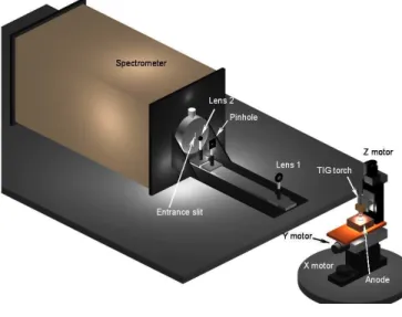
The experimental apparatus consist of an atmospheric pressure torch (described extensively in Fanara, 2003; Vilarinho and Scotti, 2004; and Fanara, 2005) run in open air (Fig.2).
An arc series-regulated power supply (350 A, 110 V) provides a uniform and stable output of arc currents (output ripple less than 0.1 A). The arc is struck by contacting the cathode tip and the anode and thereafter lifting the tip up to the desired electrode spacing, kept constant at 5 mm in this work to adhere to the TIG arc length conditions prevailing in the literature. The same applies to the choice of the shielding argon flow rate (10 slm = 2.97 x 10⁻⁴ kg s-1) and to the specified tip geometry (60° included angle). The arc setup includes linear stages which permit the precision positioning of the arc with respect to the optical detection system. The optical arrangement is shown in Fig. 3 and consists of a Czerny-Turner monochromator (1 m focal length, 1200 g/mm, 0.1 Å spatial resolution) equipped with a CCD detector.
Figure 2. Picture of the experimental set up.
500 500 87.5 35
Spectrometer entrance Diaphragm
Arc
Pinhole Ø 50 µm Lens 1
F.L. = 250 mm
Lens 2 F.L. = 25 mm Diaphragm
2
5
4
.4
Quotas in mm Scale:
----Figure 3. The arc light path in the optical system.
The method employed for the temperature determination was initially proposed by Fowler and Milne (Fowler and Milne, 1923a and 1923b) and employed among the others by Olsen (1959) and Thornton (1993a and 1993b). For plasmas in LTE and at constant pressure, Equation 12 passes through a maximum at a temperature called the normal temperature.
( )
4πλ ( )
m
E k T m
mr mr mr m
mr m
N T hc
I k A g e
Z T
−
= (12)
where Imr is the experimental spectral intensities, kmr is a constant that
represents radiation losses between the arc and monochromator, h is the Planck’s constant, c is the light speed, Amr is the spontaneous
transition probability, gm is the statistical weight, Nm is the particle
density, Em is the excitation energy, k is the Boltzmann’s constant, T is
the temperature, λmr is the wavelength, Zm is the partition function. The
indexes m and r represent the transitional states from where the photon is emitted.
The first step of the Fowler-Milne method is to choose a non self-adsorbed line (Bober and Tankin, 1969), collect the spectra and determine the peak or integral intensity for each point through a horizontal plane (Fig. 4a-c). An Abel Inversion, Fig. 4d, permits to compare the normalized emission coefficient profile to the profile obtained by Eq. (12) (Fig. 4e). Once the maximum of the experimental inverted curve is found, the emission coefficient values towards the centre of the arc (in Fig. 4d, R < 1.5 mm) are compared with the right side after the maximum of the Fowler-Milne curve, i.e., higher temperatures (depending on the line being used). Conversely, the maximum of the experimental emission coefficients past the maximum (in Fig. 4d, R > 1.5 mm) should be compared to the left side of the Fowler-Milne curve. As the maximum intensity does not occur in the arc centre, this method is also called off-axis maximum method.
The Fowler-Milne method has the advantage of eliminating the use of transition probabilities and avoids apparatus calibration. However, the partition functions and number densities of the species must be calculated, although the ratio Nm(T)/Zm(T) is almost
independent of the temperature, so that only a small uncertainty in T results (Murphy, 1994). As noticed by several authors (Olsen, 1959; and Thornton, 1993b) the method is limited to the lower measurable temperatures of 9,000-10,000 K for argon using Ar I lines. This is due to the abrupt decay of the normalized intensity above 10,000 K (Fig. 4). For this reason, the lowest isotherm prevailing in literature is between 9,000 and 10,000 K.
Results
Figure 5 reports the temperatures obtained for the case of (a) I = 100 A and (b) 200 A. In the latter case, the determination obtained by using the two lines in Tab. 1 gives a perception about the line dependency of the temperature (and thus an indirect measure of its uncertainty).
The curves were built using a least square fit on 50 x 25 points matrices: 50 radial points for each of the 25 z planes to yield 1250 experimental points per arc. With the exception of a single previous experiment (Thornton, 1993b), this is a high an almost unprecedented number of points. As the arc length is 5 mm and the radial measurements extended up to 5 mm from the axis, the size of each two-dimensional “cell”, which determines the spatial resolution, is thus δr = 100 µm by δz = 200 µm. The three-dimensional cell centered on each experimental point has a volume of the order of 2⋅(100 µm)3 = 2⋅10-12 m-3, and considering a typical electron density of 1023 m-3 (at I = 200 A) it contains ~1011 particles.
Differences between errors in the two lines used are less than 0.01 %. An average of 2.0 % uncertainty on the temperature was evaluated in this work with the maximum error of 2.93 % found at 22,000 K.
These temperature maps shown here for illustration, should be used with some caution because of some underlying hypotheses made for the final two-dimensional least square fit step (which depends on the stiffness used for the distribution). Maps reported in earlier works (Olsen, 1959, for instance) seems to be drawn by hand. For this reason, in any subsequent quantitative analysis we use non-conditioned data (e.g. without this last fitting step procedure) for the temperatures and the derived parameter, all used as radial distributions of ‘raw’ data.
(a)
(b)
Figure 5. Electron temperature from OES (a) 100A (b) 200A. For the latter, the isotherms obtained from the two emission lines λλλλ = 696.54 nm and λλλλ = 706.72 nm are compared.
Table 1. Spectral lines used here (after Fuhr, 2000).
Type Wavelength [nm]
Amr
[108⋅s-1]
Em – Er
[eV] – [eV] gm – gr Ar I 696.5430 6.39⋅10-02 11.54835 – 13.32786 5 – 3 Ar I 706.7217 3.80⋅10-02 11.54835 – 13.30223 5 – 5
0.0 0.4
0 .8 1. 2
1.6 2 .0
2 .4 2.8
3.2 3 .6
4.0 4 .3
4 .7
r (mm)
0.0 0.4 0.8 1.2 1.6 2.0 2.4 2.8 3.2 3.6 4.0 4.4 4.8
z
(
m
m
)
100 A
1020
20
(a)
0.0 0.4
0 .8 1. 2
1.6 2 .0
2 .4 2.8
3.2 3 .6
4.0 4 .3
4 .7
r (mm)
0.0 0.4 0.8 1.2 1.6 2.0 2.4 2.8 3.2 3.6 4.0 4.4 4.8
z
(
m
m
)
200 A
10 20
30 40
(b)
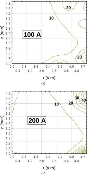
Figure 6. Debye number for pure argon arc at (a) I = 100 A and (b) I = 200 A.
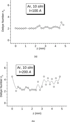
It is worth looking at this result in more detail. Figure 8 reports the radial distribution of the Debye number at different heights from the anode for the two cases I = 100 A and I = 200 A. Figure 8 reports the axial distribution of the same quantity in the two cases.
The following observations are possible:
i The axial nD is lower for the lower arc current, I = 100
(Fig. 8);
ii nD shows a local maximum close to the axis, whereas a
minimum occurs beyond 1 mm from the axis cf. Fig. 7a and b;
iii At I = 100 A, the maximum occurs at the highest z coordinate, thus closer to the cathode as shown in Fig. 8a; at I = 200 A, the axial values are more scattered;
iv Considering that the inner region of the arc is usually assumed in LTE, it is striking that here nD ~7 (at 100 A) and
nD ~4 (at 200 A). A further rise occurs at higher radial
distances but still nD ~10;
v The inner region extending for 3 to 4 mm at these arc currents is considered to be comparable with the current carrying region. So the question is whether the current carrying region may be considered and quasi-neutral ‘bulk’ plasma in LTE as it is usually assumed in literature (Allum 1983; Haidar, 1997; and Sansonnes et al., 2000).
0 1 2 3 4
2 3 4 5 6 7
n
D, z=4.8 mm
nD, z=2.4 mm
n
D, z=3.6 mm
nD, z=1.2 mm
I=100 A
nD
r (mm)
(a)
0 1 2 3 4
2 3 4 5 6
7 n
D, z=3.6 mm
nD, z=4.8 mm nD, z=2.4 mm nD, z=1.2 mm
I=200 A
nD
r (mm)
(b)
Figure 7. Radial distribution of the Debye number at different heights z from the anode (a) 100 A (b) 200 A.
Discussion
It is possible to quantify the departure from quasi-neutrality by computing the ratio
δn/ne
.
(ni-ne)/ne = [ε0/(nee)]∇2V (13)obtained from the one-dimensional Poisson’s equation, provided information on the potential E or the electric field is available. The axial component of the latter can be evaluated by using Ohm’s law integrated on the arc cross-section; for the total measured arc current I:
0
2π σ( )
R
I= E r
∫
r dr (14)0
/ 2π σ[ ( )]
R
E=I
∫
r T r dr (15)where the electrical conductivity σ(T) is obtained for every position r as a function of temperature by using Murphy’s data for argon in LTE (Murphy, 2000). The upper limit for integration, R is the radius of the minimum isotherm allowing LTE (T ≥ 9,000 K); or the minimum isotherm from the spectroscopic data available for the maximum possible number of points. Those isotherms are indicated in Fig. 9 and the choice of the radius, not always straightforward, has been made to keep the uncertainty within the error on the temperature (maximum evaluated as 300 K). The result is plotted in Fig. 9a and 9b for the two cases I = 100 A and I = 200 A.
0 1 2 3 4 5
0 2 4 6
z (mm)
D
e
b
y
e
N
u
m
b
e
r
nD
Ar, 10 slm I=100 A
(a)
0 1 2 3 4 5
0 2 4
6 Ar, 10 slm
I=200 A
D
e
b
y
e
N
u
m
b
e
r
nD
z (mm)
(b)
Figure 8 Axial distribution of the Debye number at different heights z from the anode (a) 100 A (b) 200 A.
These values are reasonably close to electric fields reported in literature (Allum, 1983). The corresponding axial δn is computed from (13) using the derivative dE/dz but taking account of the charge unbalance sign, as it is shown in Figs. 10a and 10b. It is interesting to observe that the violation of the quasi-neutrality, comparable in the two cases, is accompanied by a change of charge sign at about 1.5 mm from the anode, corresponding to the minimum in the electric field. This feature resembles the result presented in (Sansonnes et al., 2000) where a change of polarity in the potential is predicted, for I = 200 A, from positive to negative, however at a distance z ~ 2.8 mm from the anode.
0 1 2 3 4 5 6
0.2 0.4 0.6 0.8 1.0 1.2 1.4 1.6 1.8
(isotherm: 9,600 (300) K)
Ar, 10 slm I=100 A
E
(
V
/m
m
)
z (mm)
(a)
0 1 2 3 4 5 6
0.2 0.4 0.6 0.8 1.0 1.2 1.4 1.6 1.8
(isotherm: 10,250 (300) K)
Ar, 10 slm I=200 A
E
(
V
/m
m
)
z (mm)
(b)
Figure 9. Axial electric field at different heights z from the anode (a) 100 A (b) 200 A. The two isotherm used for the computation are indicated.
The order of this result, δn~ 107 m-3, is the value of the difference evaluated within one “experimental cell”, containing on average ~1011 particles. It means that the resulting electric field is
determined by a charge unbalance of 107 particles over a total of 1011 particles, i.e. on average, 1 over 104 charges are ‘unbalanced’.
These unbalanced charges generate the field E, seen as a spatial average over the cell. Stated differently, in between two experimental points along the axis, spaced 200 µm, there are ~104/2=5,000 Debye spheres, each containing only 2 (100 A) or 3 (200 A) charges; each of these spheres constitute an ensemble of Debye spheres contributing to the average field ‘seen’ in between the two experimental points. The micro-fields over region smaller than these may be considerably higher (leading to higher potentials and higher ∆V) but are not accessible experimentally.
Conclusions
preserve the electrical (quasi-) neutrality required for a discharge to be called a plasma. In particular, the hottest regions of these arcs, which are supposed to be the closest to LTE are the ones which show the lowest value of nD. The shielding of the potential in these regions is therefore incomplete. This opens to question the simultaneous attainability of LTE and quasi-neutrality.
0 1 2 3 4 5
-3x10⁷ -2x10⁷ -1x10⁷ 0 1x10⁷ 2x10⁷ 3x10⁷
ne-ni
ne
-n
i
z (mm)
Ar, 10 slm I=100 A
(a)
0 1 2 3 4 5
-3x10⁷
-2x10⁷ -1x10⁷ 0 1x10⁷ 2x10⁷
3x10⁷
ne-ni
Ar, 10 slm I=200 A
z (mm)
ne
-n
i
(b)
Figure 10. Axial distribution of the ratio (Eq. (13)) at different heights z from the anode (a) 100 A (b) 200 A.
Acknowledgement
This work was funded by EPSRC grant Nr. GR/L8 2281, and Nr. GR/NB2648/01 and by CAPES, in Brazil. The authors wish to acknowledge the extensive use of equilibrium data for pure argon provided by Anthony B. Murphy of CSIRO, Australia.
References
Allum, C.J., 1983, “Power dissipation in the column of a TIG arc”, Journal of Physics D: Applied Physics, Vol.16, pp. 2149-2165.
Benilov, M.S., 1999, “Modeling of a non-equilibrium cylindrical column of a low-current arc discharge”, IEEE Transactions on Plasma Science, Vol. 27, N. 5, pp. 1458.
Bober, L. and Tankin, R.S., 1969, “Emission and Absorption Measurements on a Strongly Self-absorbed Argon Atomic Line”, J. Quant. Spectrosc. Radiat. Transfer, Vol. 9, pp. 855-874.
Chen, F.F., 1984, “Introduction to Plasma Physics and controlled fusion, Vol. 1: Plasma Physics”, New York, London: Plenum Press.
Cram, L.E., Poladian, L., Roumeliotis, G., 1988, “Departures from equilibrium in a free-burning argon arc”, Journal of Physics D: Applied Physics, Vol. 21, pp. 418.
Eliezer, S., 2002, “The Interaction of High-Power Lasers with Plasmas”. Series in Plasma Physics, ed. S. Cowley, Scott, P., Wilhelmsson, H., IOP Publishing.
Fanara, C., 2003, “A Langmuir multi-probe system for the characterization of atmospheric pressure arc plasmas”, Ph.D. Thesis. SIMS, Cranfield University.
Fanara, C., 2005, “Sweeping electrostatic probes in atmospheric pressure arc plasmas”, IEEE Transactions on Plasma Science, Vol.33, N.3, pp. 1072-1081.
Fowler, R.H. and Milne, E. A., 1923b, “The maxima of absorption lines in stellar spectra”, Monthly Notices Roy. Astron. Soc, Vol. 84, pp. 499-515.
Fowler, R.H. and Milne., E. A., 1923a, “The intensities of absorption lines in stellar spectra, and the temperatures and pressures in the reversing layers of stars”, Monthly Notices Roy. Astron. Soc, Vol.83, pp. 403-424.
Fuhr, J.R., 2000, “NIST Atomic Spectra Database”, Gaithersburg, M.D, Available in http://physics.nist.gov/cgi-bin/AtData/lines_form
Golant, V.E., Zilinskij, A.P., Sacharov, S.E., 1983, “Fondamenti di Fisica dei Plasmi”, MIR Moscow-ER Rome (Italian translation).
Goldbach, C., Nollez, G., Popovic, S., Popovic, M., 1978, “Electrical conductivity of high pressure ionized Argon”, Z. Naturforsch, Vol. 33a, pp. 11-17.
Günther, K., Lang, S., Radtke, R., 1983, “Electrical conductivity and charge carrier screening in weakly non-ideal argon plasmas”, Journal of Physics D: Applied Physics, Vol. 16, pp. 1235-1243.
Günther, K., Popovic, M.M., Popovic, S.S., Radtke, R., 1976, “Electrical conductivity of highly ionized dense hydrogen plasma: II. Comparison of experiment and theory”, Journal of Physics D: Applied Physics, Vol 9, pp. 1139-1147.
Haddad, G.N., Farmer, A.J.D., 1984, “Temperature determinations in free burning arc: I. Experimental techniques and results in argon”, Journal of Physics D: Applied Physics, Vol.17, p. 1189-1196.
Haddad, G.N., Farmer, A.J.D., Kovyta, P., Cram, L.E., 1986, “Physical processes in gas-Tungsten arcs”, IEEE Transactions on Plasma Science, Vol. PS-14, p. 333.
Haidar, J., 1997, “Departures from local thermodynamical equilibrium in high-current free burning arcs in air”, Journal of Physics D: Applied Physics, Vol.30, pp. 2737-43.
Murphy, A.B., 1994, “Modified Fowler-Milne method for the spectroscopic measurement of temperature and composition of multielement thermal plasmas”, Rev. Sci. Instrum., Vol.65, No.11, pp. 3423-3427.
Murphy, A.B., 1997, “Transport coefficients of Helium and Argon-Helium plasmas”. IEEE Transactions on Plasma Science, Vol.25, No.5, pp. 809-814.
Murphy, A.B., 2000, “Private communication”.
Olsen, H.N., 1959, “Thermal and electrical properties of an Argon plasma”, The Physics of Fluids, Vol. 2, No.6, pp. 614-623.
Sansonnes, L., Haidar, J., Lowke JJ., 2000, “Prediction of properties of free burning arcs including effects of ambipolar diffusion”. Journal of Physics D: Applied Physics, Vol. 33, pp. 148-157.
Thornton, M.F., 1993a, “Spectroscopic Determination of Temperature distributions for a TIG arc”, PhD Thesis, Cranfield University.
Thornton, M.F., 1993b, “Spectroscopic determination of temperature distributions for a TIG arc”, Journal of Physics D: Applied Physics, Vol. 26, pp. 1432-1438.