ISSN 0101-8205 / ISSN 1807-0302 (Online) www.scielo.br/cam
A special class of continuous general linear methods
D.G. YAKUBU1∗, A.M. KWAMI and M.L. AHMED Mathematical Sciences Programme, Abubakar Tafawa Balewa University,
PMB 0248, Bauchi, Nigeria
E-mails: [email protected] / [email protected] / [email protected]
Abstract. We consider the construction of a class of numerical methods based on the general matrix inverse [14] which provides continuous interpolant for dense approximations (output). Their stability properties are similar to those for Runge-Kutta methods. These methods provide a unifying scope for many families of traditional methods. They are self-starting, to change stepsize
during integration is not difficult when using them. We exploited these properties by first obtaining the direct block methods associated with the continuous schemes and then converting the block methods into uniformly A-stable high order general linear methods that are acceptable for solving stiff initial value problems. However, we will limit our formulation only for the step numbers
k=2,3,4. From our preliminary experiments we present some numerical results of some initial value problems in ordinary differential equations illustrating various features of the new class of
methods.
Mathematical subject classification: 65L05.
Key words:block method, continuous scheme, general linear method, matrix inverse.
1 Introduction
General linear methods emerged as a result of the desire to obtain a wider general-ization of a large family of traditional numerical methods for ordinary differential equations. They were first introduced by [2] as a unifying theory for studying
#CAM-356/11. Received: 17/IV/11. Accepted: 24/II/12. *Corresponding author.
stability, consistency and convergence for a wide variety of traditional methods. Their formulations include both the multi-stage nature of Runge-Kutta methods as well as the multi-value nature of linear multistep methods which also allows for many generalizations of the traditional methods [4]. General linear meth-ods, however, have not yet gained the popularity they deserve despite they have been in existence for over forty years. Their discovery opened up many possi-bilities of obtaining essentially new methods that were neither Runge-Kutta nor linear multistep methods which exist practically and have advantages over the traditional methods. For example “Almost Runge-Kutta” methods [5], two step Runge-Kutta methods [9, 12] and Hybrid methods [10] etc. Some of the reasons for their generalizations are:
• Runge-Kutta methods, which are always termed to be the best known one-step methods, have been regarded as expensive because of their mul-tistage structure (multiple function calls in each time step [7]). Runge-Kutta methods use more function evaluations to attain the same accuracy as compared with the linear multistep methods. The implementation costs for implicit Runge-Kutta methods (Gauss, Lobatto and Radau) present obstacle to finding cheap implementation because of the structure of the coefficient matrix Ain Butcher’s array, which has a pair of complex con-jugate eigenvalue. For both explicit and implicit Runge-Kutta methods it is very difficult to estimate errors for variable stepsizehand order p[7].
• Linear multistep methods, on the other hand suffer the disadvantages of poor stability property as the step number increases with accuracy and requiring additional starting values with constant step size from other one-step methods. For the A-stability which is a desirable property for stiff problems, order is limited by Dahlquist barriers to two.
2 General linear methods
The name “general linear methods” applies to a large family of numerical meth-ods for ordinary differential equations. Runge-Kutta methmeth-ods and linear multi-step methods are examples of these methods. Further, a general linear method used for the numerical solution of system of initial value problem in ordinary differential equations of the form
y′ = f(x,y),y(x0)=y0, a≤ x ≤b, (1)
is both multistage as the Runge-Kutta methods and multivalue as the linear multistep methods. In the general linear methods we denote the internal stage values of step numbernby
Y1[n],Y2[n], . . . ,Ys[n]
and the derivatives evaluated at these steps by
f(Y1[n]), f(Y2[n]), . . . , f(Ys[n]).
At the start of the step numbern,r quantities denoted by
y1[n−1],y2[n−1], . . . ,yr[n−1]
are available from approximations computed in stepn−1. Corresponding quan-tities
y1[n],y2[n], . . . ,yr[n]
are evaluated in the step numbern. Introducing the vectors
Y[n], f(Y[n]),y[n−1] and y[n]
we can write them as follows:
Y[n]=
Y1[n] Y2[n]
.. .
Ys[n]
, f(Y[n])=
f(Y1[n])
f(Y2[n]) .. .
f(Ys[n])
, y[n−1]=
y1[n−1] y2[n−1]
.. .
yr[n−1]
, y[n]=
y[1n] y[2n]
.. .
whererdenotes quantities as output from each step and input to the next step and
sdenotes stage values used in the computation of the stepY1[n],Y2[n], . . . ,Y[n]
s .
If the stepsize is h then the quantities imported into and evaluated in step numbernare related by the relations
Y[n]=h(A⊕Im)f(Y[n])+(U⊕Im)y[n−1], y[n]=h(B⊕Im)f(Y[n])+(V ⊕Im)y[n−1],
wheren =1,2, . . . ,N;I is the identity matrix of size equal to the differential equation system to be solved andmis the dimension of the system. Also⊕is the Kronecker product of two matrices. For simplicity, we write the method as:
Y[n]=h A f(Y[n])+U y[n−1],
y[n]=h B f(Y[n])+V y[n−1], (2) and the coefficients of the method, that is, the elements of A,B,U andV as a partitioned(s+r)×(s+r)matrix:
M=
"
A U B V
#
.
This formulation of general linear methods was introduced by Burrage and Butcher [1]. The structure of the leading coefficient matrix Awhich is similar to that of theAmatrix in Runge-Kutta methods, determines the implementation cost of these methods. TheV matrix determines the stability of these methods. The Bmatrix gives the weights. TheU matrix is simplye. The vectory[n]can
have a very general structure. That is to say the quantities could approximate the solution and the derivatives of various previous points, backward difference approximations to the derivatives or approximations to a Nordsieck vector, all of which are common choices in linear multistep methods. In the case of the Runge-Kutta methods,y[n] could be an approximation to y
nor perturbation of ynusing the generalization to effective order.
Definition 2.1. [8] For a general linear method (A,U,B,V) the ‘stability matrix’ M(z)is defined by
and the characteristic polynomial is given by
8(ω,z)=det(ωI −M(z)).
Definition 2.2. [8] If a general linear method (A,U,B,V) has a stability function which takes the special form:
8(ω,z)=ωr−1(ω−R(z))
where the rational function R(z)is known as the ‘stability function’ of the method, then the method is said to have Runge-Kutta stability.
Definition 2.3. [8]A general linear method(A,U,B,V)is A-stable if for all z ∈C−, I −z A is non-singular and M(z)is a stability matrix.
For methods with this property the step size is never restricted by stability on linear constant coefficient problems, regardless of the stiffness.
Definition 2.4. [6] A general linear method(A,U,B,V) is L-stable if it is A-stable andρ(M(∞))=0or the stronger condition M(∞)=0.
3 Derivation technique
A particularly useful class of discrete methods for the numerical integration of (1) is the class of linear multistep methods of the form
yn+k = k
X
j=0
φjyn+j+h k
X
j=0
ψjfn+j (3)
wherek > 0 is the step number, φj, j = 0,1, . . . ,t−1; ψj, j = 0,1, . . ., s −1 are the coefficients of the discrete scheme, with yn+j = y(xn+j),j =
0,1, . . . ,k −1, h is assumed (for simplicity of the analysis) to be a constant step-size given by
h=xn+1−xn;n =0,1, . . . ,N;h N =b−a;
and a set of equally spaced points on the integration interval also given by
To obtain its continuous formulation, in the sense of [14] which was a gen-eralization of [13], we consider a polynomial y(x)of degree p = t +s −1,
t>0, s >0, of the form
y(x)= t−1
X
j=0
φj(x)yn+j+h s−1
X
j=0
ψj(x)f(xj,y(xj)) (4)
defined over thek-steps ,x ∈ {xn,xn+k}such that it satisfies the conditions
y(xn+j)=yn+j, j ∈ {0,1, . . . ,t−1} (5)
y′(xj)= f(xj,y(xj)), j =0,1, . . . ,s−1, (6)
whereφj(x)andψj(x)are assumed polynomials of the form:
φj(x)= t+s−1
X
i=0
φj,i+1xi, j ∈ {0,1, . . . ,t−1}; (7)
hψj(x)=h t+s−1
X
i=0
ψj,i+1xi, j=0,1,2, . . . ,s−1, (8)
xn+j in (5) are t(t > 0) arbitrarily chosen interpolation points taken from {xn,xn+k} and the collocation points xj, j = 0,1, . . . ,s −1 in (6) also
be-long to {xn,xn+k}. From the interpolation and collocation conditions (5) and
(6), and the expression fory(x)in (4), the following conditions are imposed on
φj(x)andψj(x):
φj(xn+i)=δi j, j =0,1, . . . ,t−1;i=0,1, . . . ,t−1
hψj(xn+i)=0, j =0,1, . . . ,s−1;i=0,1, . . . ,t−1 (9)
and
φ′j(xi)=0, j =0,1, . . . ,t−1;i =0,1, . . . ,t−1
hψ′j(xi)=δi j, j =0,1, . . . ,s−1;i=0,1, . . . ,t−1. (10)
Next we write (9)-(10) in a matrix equation of the form
whereI is an identity matrix of appropriate dimension,
D=
1 xn x2n ∙ ∙ ∙ xnt+s−1
1 xn+1 x2n+1 ∙ ∙ ∙ x t+s−1 n+1 ..
. ... ... . .. ...
1 xn+t−1 xn2+t−1 ∙ ∙ ∙ x t+s−1 n+t−1
0 1 2xn ∙ ∙ ∙ (t+s−1)xtn+s−2 ..
. ... ... . .. ...
0 1 2xn+s ∙ ∙ ∙ (t+s−1)xtn++ss−2
(12)
and
C =
φ0,1 φ1,1 ∙ ∙ ∙ φt−1,1 hψ0,1 ∙ ∙ ∙ hψs−1,1 φ0,2 φ1,2 ∙ ∙ ∙ φt−1,2 hψ0,2 ∙ ∙ ∙ hψs−1,2
..
. ... . .. ... ... . .. ... φ0,t+s φ1,t+s ∙ ∙ ∙ φt−1,t+s hψ0,t+s ∙ ∙ ∙ hψs−1,t+s
. (13)
The matrices D andC are both of dimensions(t+s)×(t+s). It follows from (11) that the columns ofC = D−1give the continuous coefficientsφ
j(x)
andψj(x). We now derive the continuous formulation of the general linear
methods following the derivation techniques discussed in Section 3.
4 The class of continuous general linear methods
in (12) becomes
D=
1 xn xn2 x
3
n x
4
n x
5 n
1 xn+1 xn2+1 x 3
n+1 xn4+1 x 5 n+1
1 xn+2 xn2+2 x 3 n+2 x
4 n+2 x
5 n+2
0 1 2xn 3x2n 4x
3
n 5x
4 n
0 1 2xn+1 3x2n+1 4x 3 n+1 5x
4 n+1
0 1 2xn+2 3x2n+2 4x 3 n+2 5x
4 n+2
. (14)
Inverting the matrix in (14) once, using computer algebra, for example, Maple or Matlab software package, give rise to the following continuous scheme
y(x) = φ0(x)yn+φ1(x)yn+1+φ2(x)yn+2 + ψ0(x)fn+ψ1(x)fn+1+ψ2(x)fn+2
, (15)
where
φ0(x) =
3ζ5−17hζ4+33h2ζ3−23h3ζ2+4h5
4h5
,
φ1(x) =
ζ4−4hζ3+4h2ζ2 h4
,
φ2(x) =
−3ζ5+13hζ4−17h2ζ3+7h3ζ2
4h5
,
ψ0(x) =
ζ5−6hζ4+13h2ζ3−12h3ζ2+4h4ζ
4h4
,
ψ1(x) =
ζ5−5hζ4+8h2ζ3−4h3ζ2 h4
,
ψ2(x) =
ζ5−4hζ4+5h2ζ3−2h3ζ2
4h4
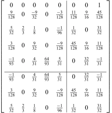
Evaluating the continuous scheme in (15), we first obtain the block method associated with the continuous scheme and we converted the block method into uniformly accurate order general linear method:
0 0 0 0 0 0 0 1
9 128 0 −9 32 0 −3 128 11 128 9 16 45 128 5 32 2 3 1 8 0 −1 96 1 32 0 31 32 3 128 0 9 32 0 −9 128 45 128 9 16 11 128 −1 93 0 4 31 64 93 5 31 0 32 31 −1 31 −1 93 0 4 31 64 93 5 31 0 32 31 −1 31 3 128 0 9 32 0 −9 128 45 128 9 16 11 128 5 32 2 3 1 8 0 −1 96 1 32 0 31 32 . (16)
We plotted the region of absolute stability of the general linear method (16) using the method used in [9] as shown below:
Fork=3, the matrix Din (12) takes the following form: D=
1 xn xn2 x
3 n x 4 n x 5 n x 6 n x 7 n
1 xn+1 xn2+1 x 3 n+1 x
4 n+1 x
5 n+1 x
6 n+1 x
7 n+1
1 xn+2 xn2+2 xn3+2 xn4+2 xn5+2 xn6+2 xn7+2
1 xn+3 xn2+3 x 3 n+3 x
4 n+3 x
5 n+3 x
6 n+3 x
7 n+3
0 1 2xn 3x2n 4x
3
n 5x
4
n 6x
5
n 7x
6 n
0 1 2xn+1 3x2n+1 4x 3 n+1 5x
4 n+1 6x
5 n+1 7x
6 n+1
0 1 2xn+2 3x2n+2 4x 3 n+2 5x
4 n+2 6x
5 n+2 7x
6 n+2
0 1 2xn+3 3x2n+3 4x 3 n+3 5x
4 n+3 6x
5 n+3 7x
6 n+3
(17)
and we obtain
y(x) = φ0(x)yn+φ1(x)yn+1+φ2(x)yn+2+φ3(x)yn+3 + ψ0(x)fn+ψ1(x)fn+1+ψ2(x)fn+2+ψ3(x)fn+3
. (18)
as the continuous scheme, where also
φ0(x)= "
11ζ7−129hζ6+602h2ζ5−1410h3ζ4+1691h4ζ3−873h5ζ2+108h6
108h7
#
,
φ1(x)= "
ζ7−10hζ6+37h2ζ5−60h3ζ4+36h4ζ3
4h7
#
,
φ2(x)= "
−ζ7+11hζ6−46h2ζ5+90h3ζ4−81h4ζ3+27h5ζ2
4h7
#
,
φ3(x)= "
−11ζ7+102hζ6−359h2ζ5+600h3ζ4−476h4ζ3+144h5ζ2
108h7
#
,
ψ0(x)= "
ζ7−12hζ6+58h2ζ5−144h3ζ4+193h4ζ3−132h5ζ2+36h6ζ
36h6
#
ψ1(x)= "
ζ7−11hζ6+47h2ζ5−97h3ζ4+96h4ζ3−36h5ζ2
4h6
#
,
ψ2(x)= "
ζ7−10hζ6+38h2ζ5−68h3ζ4+57h4ζ3−18h5ζ2
4h6
#
,
ψ3(x)= "
ζ7−9hζ6+31h2ζ5−51h3ζ4+40h4ζ3−12h5ζ2
36h6
#
.
Evaluating the continuous scheme (18) we obtain the block method first and then converted the block method into general linear method:
0 0 0 0 0 0 0 0 0 0 1
25 512 0 225 512 0 −75 512 0 −5 512 61 1536 125 512 225 512 425 1536 155 1305 768 1305 −45 1305 0 −162 1305 0 −13 1305 31 783 5 29 0 617 783 3 512 0 81 512 0 −81 512 0 −3 512 13 512 243 512 243 512 13 512 1 405 0 81 405 256 405 81 405 0 1 405 −1
81 0 1
1 81 5 512 0 75 512 0 225 512 0 −25 512 425 1536 225 512 125 512 61 1536 −39 3085 0 −495 3085 0 −135 3085 2304 3085 465 3085 0 783 617 −135 617 31 617 −39 3085 0 −495 3085 0 −135 3085 2304 3085 465 3085 0 783 617 −135 617 31 617 5 512 0 75 512 0 225 512 0 −25 512 425 1536 225 512 125 512 61 1536 1 405 0 81 405 256 405 81 405 0 1 405 −1
81 0 1
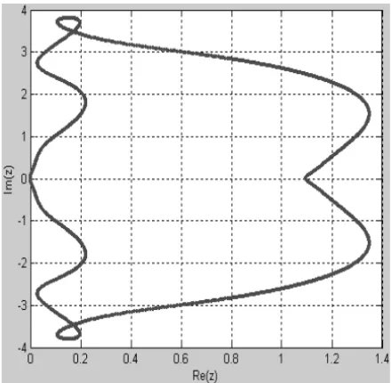
1 81 155 1305 768 1305 −45 1305 0 −162 1305 0 −13 1305 31 783 5 29 0 617 783 . (19)
Figure 2 – Region of absolute stability of the general linear method (19).
For k = 4, the matrix D in (12) and the polynomial equation in (4) are re-spectively:
D=
1 xn xn2 xn3 xn4 xn5 xn6 xn7 x8n xn9 1 xn+1 xn2+1 xn3+1 xn4+1 xn5+1 xn6+1 xn7+1 xn8+1 x9n+1 1 xn+2 xn2+2 xn3+2 xn4+2 xn5+2 xn6+2 xn7+2 xn8+2 x9n+2
1 xn+3 xn2+3 xn3+3 xn4+3 xn5+3 xn6+3 xn7+3 xn8+3 x9n+3 1 xn+4 xn2+4 xn3+4 xn4+4 xn5+4 xn6+4 xn7+4 xn8+4 x9n+4 0 1 2xn 3x2n 4x3n 5xn4 6x5n 7xn6 8x7n 9x8n 0 1 2xn+1 3x2n+1 4x3n+1 5x4n+1 6x5n+1 7x6n+1 8x7n+1 9x8n+1
0 1 2xn+2 3x2n+2 4x3n+2 5x4n+2 6x5n+2 7x6n+2 8x7n+2 9x8n+2 0 1 2xn+3 3x2n+3 4x3n+3 5x4n+3 6x5n+3 7x6n+3 8x7n+3 9x8n+3 0 1 2xn+4 3x2n+4 4x3n+4 5x4n+4 6x5n+4 7x6n+4 8x7n+4 9x8n+4
and
y(x)=φ0(x)yn+φ1(x)yn+1+φ2(x)yn+2+φ3(x)yn+3+φ4(x)yn+4 +ψ0(x)fn+ψ1(x)fn+1+ψ2(x)fn+2+ψ3(x)fn+3+ψ4(x)fn+4
(21)
where
φ0(x)=
25ζ9−494hζ8+4130h2ζ7−18980h3ζ6+52025h4ζ5 −85862h5ζ4+80620h6ζ3−34920h7ζ2+3456h9
3456h9
,
φ1(x)=
5ζ9−92hζ8+701h2ζ7−2846h3ζ6+6572h4ζ5 −8456h5ζ4+5376h6ζ3−1152h7ζ2
108h9
,
φ2(x)=
ζ8−16hζ7+102h2ζ6−328h3ζ5+553h4ζ4−456h5ζ3+144h6ζ2
16h8
,
φ3(x)=
−5ζ9+88hζ8−637h2ζ7+2446h3ζ6−5356h4ζ5 +6664h5ζ4−4352h6ζ3+1152h7ζ2
108h9
,
φ4(x)=
−25ζ9+406hζ8−2722h2ζ7+9748h3ζ6−20089h4ζ5 +23758h5ζ4−14892h6ζ3+3816h7ζ2
3456h9
,
ψ0(x)=
ζ9−20hζ8+170h2ζ7−800h3ζ6+2273h4ζ5−3980h5ζ4 +4180h6ζ3−2400h7ζ2+576h8ζ
576h8
,
ψ1(x)=
ζ9−19hζ8+151h2ζ7−649h3ζ6+1624h4ζ5 −2356h5ζ4+1824h6ζ3−576h7ζ2
36h8
ψ2(x)=
ζ9−18hζ8+134h2ζ7−532h3ζ6+1209h4ζ5 −1562h5ζ4+1056h6ζ3−288h7ζ2
16h8
,
ψ3(x)=
ζ9−17hζ8+119h2ζ7−443h3ζ6+944h4ζ5 −1148h5ζ4+736h6ζ3−192h7ζ2
36h8
,
ψ4(x)=
ζ9−16hζ8+106h2ζ7−376h3ζ6+769h4ζ5 −904h5ζ4+564h6ζ3−144h7ζ2
576h8
,
Evaluating the continuous scheme in (21) we obtain the block method which was converted to general linear method:
0 0 0 0 0 0 0 0 0 0 0 0 0 1
1225
32768 0 −20481225 0 −81923675 0 −2048245 0 32768−175 1966084675 15196144 12254096 12256144 19660845325 741
9488 9216 20755 −
111 593 0 −
963 2372 0 −
363
2965 0 − 381 66416 481 18976 145 593 108 593 0 10399 18976 75 32768 0 225 2048 0 −2025 8192 0 −75 2048 0 −45 32768 411 65536 175 2048 2025 4096 825 2048 725 65536 11
5184 0 10821 256405 163 0 324−1 0 2880−1 34565 324−1 0 17121728 10368113 45 32768 0 75 2048 0 2025 8192 0 −225 2048 0 −75 32768 725 65536 825 2048 2025 4096 175 2048 411 65536 −3 8560 0 −1 321 0 81 428 1024 1605 21 107 0 11 5136 −113 10272 0 108 107 1 321 −5 3424 175
32768 0 2048245 0 36758192 0 12252048 0 −327681225 19660845325 12256144 12254096 15196144 1966084675
−762 72793 0 616 51995 0 −7704 10399 0 −3552 10399 294912 363965 1482 10399 0 18976 10399 −3456 10399 −4640 10399 −481 10399 −762 72793 0 616 51995 0 −
7704 10399 0 −
3552 10399 294912 363965 1482 10399 0 18976 10399 − 3456 10399 − 4640 10399 − 481 10399 175 32768 0 245 2048 0 3675 8192 0 1225 2048 0 −1225 32768 45325 196608 1225 6144 1225 4096 1519 6144 4675 196608 −3
8560 0 321−1 0 42881 10241605 10721 0 513611 10272−113 0 108107 3211 3424−5 11 5184 0 21 108 256 405 3
16 0 − 1
5 Numerical illustrations
In order to test the methods of section 4 we present some numerical results. The absolute errors of the results obtained from computed and exact solutions at some selected mesh points are shown in Tables.
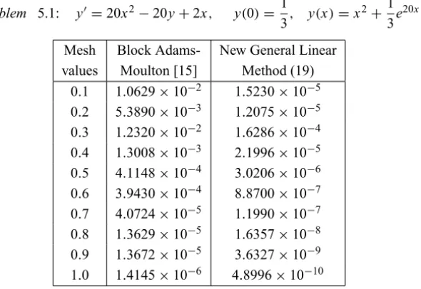
Problem 5.1: y′=20x2−20y+2x, y(0)=1
3, y(x)=x 2+1
3e 20x
Mesh Block Adams- New General Linear values Moulton [15] Method (19)
0.1 1.0629×10⁻² 1.5230×10⁻⁵ 0.2 5.3890×10⁻³ 1.2075×10⁻⁵ 0.3 1.2320×10⁻² 1.6286×10⁻⁴ 0.4 1.3008×10⁻³ 2.1996×10⁻⁵ 0.5 4.1148×10⁻⁴ 3.0206×10⁻⁶ 0.6 3.9430×10⁻⁴ 8.8700×10⁻⁷ 0.7 4.0724×10⁻⁵ 1.1990×10⁻⁷ 0.8 1.3629×10⁻⁵ 1.6357×10⁻⁸ 0.9 1.3672×10⁻⁵ 3.6327×10⁻⁹ 1.0 1.4145×10⁻⁶ 4.8996×10⁻¹⁰
Table 1 – Absolute errors of numerical solutions of Problem 5.1 with,h=0.1.
Problem 5.2: y′= −y, y(0)=1, y(x)=e−x
Mesh Block Adams- New General Linear values Moulton [15] Method (22)
0.1 2.1541×10⁻⁷ 2.5817×10⁻¹³ 0.2 6.9544×10⁻⁸ 2.3105×10⁻¹³ 0.3 2.8062×10⁻⁷ 7.4733×10⁻¹³ 0.4 4.1350×10⁻⁷ 1.2390×10⁻¹³ 0.5 2.8127×10⁻⁷ 1.1002×10⁻¹³ 0.6 4.1578×10⁻⁷ 1.1066×10⁻¹³ 0.7 4.9444×10⁻⁷ 4.1514×10⁻¹⁴ 0.8 3.7858×10⁻⁷ 3.6091×10⁻¹⁴ 0.9 4.6203×10⁻⁷ 1.2298×10⁻¹³ 1.0 5.0564×10⁻⁷ 6.3784×10⁻¹⁵
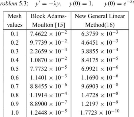
Problem5.3: y′= −λy, y(0)=1, y(0)=e−λx
Mesh Block Adams- New General Linear values Moulton [15] Method(16)
0.1 7.4622×10⁻² 6.3759×10⁻³ 0.2 9.7739×10⁻² 4.6451×10⁻³ 0.3 2.2659×10⁻⁴ 3.8855×10⁻⁴ 0.4 1.0870×10⁻² 8.4175×10⁻⁵ 0.5 7.7732×10⁻⁵ 6.9921×10⁻⁶ 0.6 1.1401×10⁻³ 1.1690×10⁻⁶ 0.7 8.8455×10⁻⁶ 9.6903×10⁻⁸ 0.8 1.1914×10⁻⁴ 1.4728×10⁻⁸ 0.9 8.8900×10⁻⁷ 1.2197×10⁻⁹ 1.0 1.2448×10⁻⁵ 1.7723×10⁻¹⁰
Table 3 – Absolute errors of numerical solutions of Problem 5.3, with stiffness ratio,λ=10000.
The fourth problem is a system of standard test problem with the exact solutions for easy comparison purposes:
y1′ = −8y1+7y2, y1(0)=1
y2′ =42y1−43y2, y2(0)=8
The coefficient matrix of this problem has two eigenvalues,λ1= −1 andλ2 = −50. The stiffness ratio is R=50. This is a mildly stiff linear problem with the exact solutions as:
y1(x)=2 exp(−x)−exp(−50x)
y2(x)=2 exp(−x)+6 exp(−50x)
Solution of problem 4.4 using BAMMk=2, with nfe=100
0 0.1 0.2 0.3 0.4 0.5 0.6 0.7 0.8 0.9 1
0 1 2 3 4 5 6 7 8
y1
y2
Solution of problem 4.4 using BAMMk=3, with nfe=100
0 0.1 0.2 0.3 0.4 0.5 0.6 0.7 0.8 0.9 1
0 1 2 3 4 5 6 7 8
y1 y2
Solution of problem 4.4 using BAMMk=4, with nfe=100
0 0.1 0.2 0.3 0.4 0.5 0.6 0.7 0.8 0.9 1
0 1 2 3 4 5 6 7 8
y1 y2
Solution of problem 4.4 using GLM (16), with nfe=100
0 0.1 0.2 0.3 0.4 0.5 0.6 0.7 0.8 0.9 1
-140 -120 -100 -80 -60 -40 -20 0 20
y1 y2
Solution of problem 4.4 using GLM (19), with nfe=100
0 0.1 0.2 0.3 0.4 0.5 0.6 0.7 0.8 0.9 1
-6 -5 -4 -3 -2 -1 0 1x 10
166
y1 y2
Solution of problem 4.4 using GLM (22), with nfe=100
0 0.1 0.2 0.3 0.4 0.5 0.6 0.7 0.8 0.9 1 -10
-8 -6 -4 -2 0 2 4 6x 10
15
y1 y2
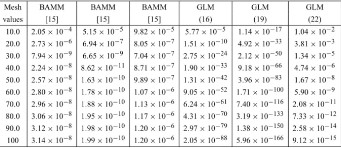
Mesh BAMM BAMM BAMM GLM GLM GLM
values [15] [15] [15] (16) (19) (22)
10.0 2.05×10⁻⁴ 5.15×10⁻⁵ 9.82×10⁻⁵ 5.77×10⁻⁵ 1.14×10⁻¹⁷ 1.04×10⁻² 20.0 2.73×10⁻⁶ 6.94×10⁻⁷ 8.05×10⁻⁷ 1.51×10⁻¹⁰ 4.92×10⁻³³ 3.81×10⁻³ 30.0 7.94×10⁻⁹ 6.65×10⁻⁹ 7.04×10⁻⁷ 2.75×10⁻²⁴ 2.12×10−50 1.34×10⁻⁵ 40.0 2.24×10⁻⁸ 8.62×10⁻¹¹ 8.71×10⁻⁷ 1.90×10⁻³³ 9.18×10−66 4.74×10⁻⁶ 50.0 2.57×10⁻⁸ 1.63×10⁻¹⁰ 9.89×10⁻⁷ 1.31×10−42 3.96×10−83 1.67×10⁻⁸ 60.0 2.80×10⁻⁸ 1.78×10⁻¹⁰ 1.07×10⁻⁶ 9.05×10−52 1.71×10−100 5.90×10⁻⁹
70.0 2.96×10⁻⁸ 1.88×10⁻¹⁰ 1.13×10⁻⁶ 6.24×10−61 7.40×10−116 2.08×10⁻¹¹ 80.0 3.06×10⁻⁸ 1.95×10⁻¹⁰ 1.17×10⁻⁶ 4.31×10−70 3.19×10−133 7.33×10⁻¹² 90.0 3.12×10⁻⁸ 1.98×10⁻¹⁰ 1.20×10⁻⁶ 2.97×10−79 1.38×10−150 2.58×10⁻¹⁴ 100 3.14×10⁻⁸ 1.99×10⁻¹⁰ 1.20×10⁻⁶ 2.05×10−88 5.96×10−166 9.12×10⁻¹⁵
Table 4 – Absolute errors of numerical solutions of the systems of equations.
Solution of example 4.5 using BAMMk=2, with nfe=100
0 5 10 15 20 25 30 35 40
-1 -0.8 -0.6 -0.4 -0.2 0 0.2 0.4 0.6 0.8 1
y(1) y(2) y(3)
Solution of example 4.5 using BAMMk=3, with nfe=100
0 2 4 6 8 10 12 14 16 18 20
-1 -0.8 -0.6 -0.4 -0.2 0 0.2 0.4 0.6 0.8 1
y(1) y(2) y(3)
Solution of example 4.5 using BAMMk=4, with nfe=100
0 5 10 15 20 25 30 35 40 -1
-0.8 -0.6 -0.4 -0.2 0 0.2 0.4 0.6 0.8 1
y(1) y(2) y(3)
Solution of example 4.5 using GLM (16), with nfe=100
0 2 4 6 8 10 12
-1 -0.8 -0.6 -0.4 -0.2 0 0.2 0.4 0.6 0.8 1
y(1) y(2) y(3)
Solution of example 4.5 using GLM (19), with nfe=100
0 2 4 6 8 10 12
-1 -0.8 -0.6 -0.4 -0.2 0 0.2 0.4 0.6 0.8 1
y(1) y(2) y(3)
Solution of example 4.5 using GLM (22), with nfe=100
0 2 4 6 8 10 12
-1 -0.8 -0.6 -0.4 -0.2 0 0.2 0.4 0.6 0.8 1
y(1) y(2) y(3)
See ODE45, ODE23, ODE113 of Matlab Work
0 2 4 6 8 10 12
-1 -0.8 -0.6 -0.4 -0.2 0 0.2 0.4 0.6 0.8 1
y(1) y(2) y(3)
Figure 4 (continuation) – Computed solutions of the system of equations in (4.5) using BAMMs [15] and the GLMs with indicated number of functions evaluations (nfe).
In Figure 4 we report the graphical plots of the Euler equation of motion for a rigid body without external forces which is one of the standard test problems of the DETest set, see Hull et al. (1972):
y′
1=y2y3, y1(0)=0 y′
Our graphical plots confirm that all the derived methods are promising in solv-ing higher order equation written in form of first order system of initial value problems. Hence for fair comparison all the methods are comparable with the ode solvers as we can see from Figure 4.
6 Conclusion
The new feature considered in this paper is the use of matrix inversion procedure which extends some conventional multistep collocation at the step points. In this way acceptable stability for stiff problems as for the Runge-Kutta methods [3] is retained. All the derived methods obtained through this approach performed remarkably well in both stiff and non-stiff systems of initial value problem in ordinary differential equations (see Tables 1, 2, 3 and 4). The plots of the fourth test problem are system of differential equations written as first order initial value problems. We plotted these solutions and compare them with the exact values, we found out that it is difficult to distinguish between the computed solutions and the exact values on the interval of integration and there is remarkable agreement over very much longer intervals (see Fig. 3). Similarly the solutions of the fifth problem were compared with ODE solvers (see Fig. 4).
Acknowledgements. The first author wishes to record his thanks to the referee for his/her constructive suggestions and comments that have led to a number of improvements to this paper.
REFERENCES
[1] K. Burrage and J.C. Butcher. Non-linear stability for a general class of
differen-tial equation methods. BIT,20(1980), 185–203.
[2] J.C. Butcher.On the Convergence of Numerical Solutions to Ordinary Differential
Equations. Math. Comp.,20(1966), 1–10.
[3] J.C. Butcher. The Numerical Analysis of Ordinary Differential Equations
(Runge-Kutta and General Linear Methods).John Wiley and Sons Ltd, Chichester (1987).
[5] J.C. Butcher. An Introduction to “Almost Runge-Kutta” methods.Appl. Numer. Math.,24(1997), 331–342.
[6] J.C. Butcher.Numerical Methods for Ordinary Differential Equations, John Wiley (2003).
[7] J.C. Butcher. General linear methods.SANUM (2005), 1–58.
[8] J.C. Butcher. Numerical Methods for Ordinary Differential Equations. Second Edition, John Wiley and Sons Ltd (2008).
[9] J.P. Chollom and Z. Jackiewicz. Construction of two step Runge-Kutta (TSRK)
methods with large regions of absolute stability. J. Compt. and Appl. Maths.,
157(2003), 125–137.
[10] C.W. Gear. Hybrid methods for initial value problems in ordinary differential
equations.SIAM, J. Numer. Anal.,2(1965), 69–86.
[11] T.E. Hull, W.H. Enright, B.M. Fellen and A.E. Sedgwick. Comparing numerical
methods for ordinary differential equations. SIAM J. Numer. Anal., 9 (1972),
609–637.
[12] Z. Jackiewicz and S. Tracogna.A general class of two step Runge-Kutta methods for ordinary differential equations.SIAM. J. Numer. Anal.,32(1996), 1390–1427. [13] I. Lie and S.P. Nørsett. Super-Convergence for multistep collocation. Math.
Comp.,52(1989), 65–80.
[14] P. Onumanyi, D.O. Awoyemi, S.N. Jatou and U.W. Sirisena.New linear multistep methods with continuous coefficients for first order initial value problems.Journal of the Nigerian Mathematical Society,13(1994), 37–51.
[15] D.G. Yakubu, P. Onumanyi and J.P. Chollom. A new family of general linear
methods based on the block Adams-Moulton multistep methods.Journal of Pure
![Figure 3 – Computed solutions of the system of equations in (4.4) using BAMMs [15]](https://thumb-eu.123doks.com/thumbv2/123dok_br/18978199.456066/17.918.227.696.130.1167/figure-computed-solutions-equations-using-bamms.webp)