Optimal design of beam-column connections of plane steel frames using the component method

Optimal design of beam-column connections of plane steel frames

using the component method

Abstract

This paper presents a methodology for optimization of beam-column connections of plane steel frames. The objective is to obtain beam- column connections mechanically more efficient and with minimum cost by determination of the optimal dimensions for the components of the connection; satisfying mechanical constraints associated with the bending moment and the rotational stiffness of the connection, without compromising its safety and integrity. Minimum and maximum limits of geometric parameters are considered, according to current regulations. Algorithms were developed to calculate the bending moment and the rotational stiffness of the connection using the “Method of Components” of Eurocode 3. Initially, it was developed a digital database with structural profiles, steel plates and commercial bolts obtained from catalogs of manufacturers, with automatic access of the data by the computational modules of structural analysis and optimization. In the optimization model, it is adopted the connection with extended end plate without stiffeners, the design variables are the dimensions and the thickness of the end plate, the diameter and the location of the bolts. In the optimization process, we use genetic algorithms with continuous and discrete variables, with the discrete variables being associated to the database. In this way, this paper presents a computational tool fully developed in MATLAB® environment for analysis and optimal design of beam-column connections for plane steel frames. Applications that show quite satisfactory results when compared with results available in the literature are presented.

Keywords

Structural optimization, Steel beam-column connections, Bolted end-plate connections.

1 INTRODUCTION

In recent years, there has been a great growth of industrial buildings and residences structured in steel. The steel structures are formed by the connection of several structural elements aiming the efficient conduction of the external forces acting on the structures for the foundations. The steel has advantageous physical and mechanical characteristics for use in the construction of plane frames, such as: good relationship between strength and structural weight, adaptability to various architectural forms, wide variety of profiles available in the market, great control in the manufacturing process in the mills which results in greater reliability in the use of these buildings.

In plane steel frames, usually the connections between the structural elements are the most critical sectors of the structure, where several internal requests occur, generating probable foci of structural insecurity. Therefore, it is indispensable that the connections are able to adequately transmit the efforts between the elements.

In conventional analysis, the beam-column connections of steel frames have been simplified by considering them to be flexible or rigid connections. Flexible connections are those in which their rotational stiffness is ideally zero, that is, the relative rotation at the end of the beam is free; the rigid connections are those in which their rotational stiffness is considered infinite, that is, there is not rotation between the connected elements. However, this consideration is an idealized form that does not reflect the real behavior of the connections. Real connections have always a certain degree of rotational stiffness and flexural resistance that generate an intermediate behavior between the two theoretical extremes mentioned, called semi-rigid connections (FAELLA et al., 2000).

Rafael da Silva Hortencioa* Gines Arturo Santos Falcónb

a _{Instituto Federal de Educação, Ciência e}

Tecnologia Fluminense – IFF, Santo Antônio de Pádua, RJ, Brasil. E-mail:

rafael.hortencio@Iff.edu.br

b _{Laboratório de Engenharia Civil (LECIV),}

Universidade Estadual do Norte Fluminense – UENF, Campos dos Goytacazes, RJ, Brasil. E-mail: gines@uenf.br

*Corresponding Author

http://dx.doi.org/10.1590/1679-78254247

Received: July 11, 2017

In Revised Form: December 27, 2017 Accepted: April 11, 2018

The simplification of the behavior of beam-column connections is still a frequent design practice, since local design standards only require verification of the flexural strength of the beams and columns in connection with the requesting stresses of the connection. Local design standards do not cover the mechanical behavior of the connection (calculation of ultimate flexural resistance, rotational stiffness and degree of rotation) (ROMANO, 2001).

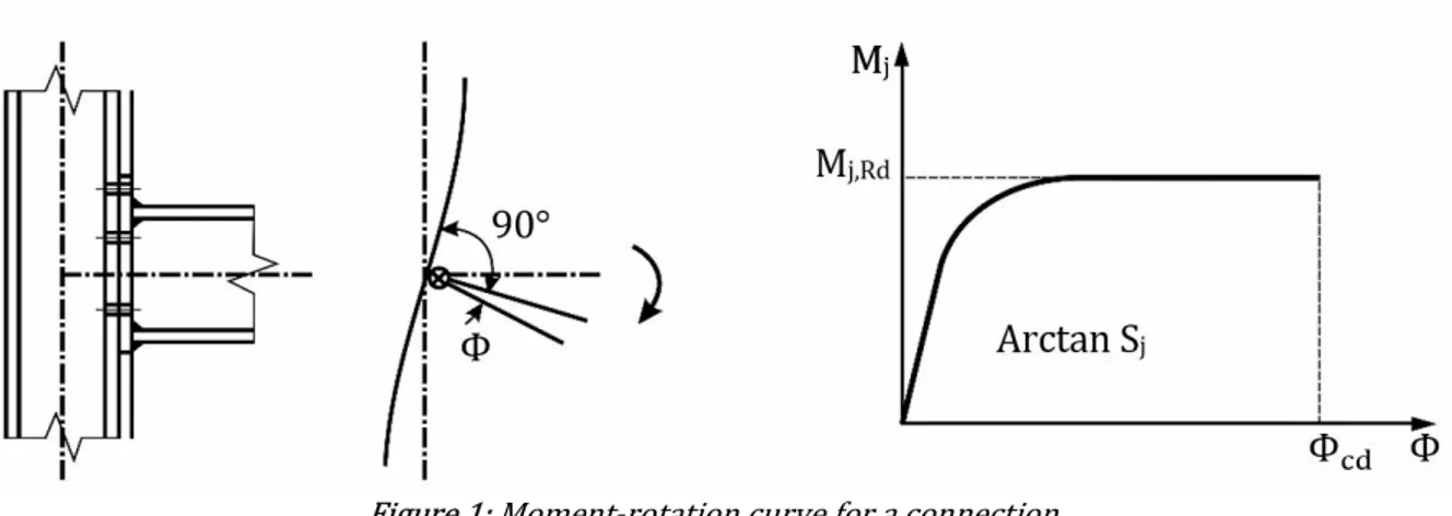
The process of structural analysis of a connection can be represented by a rotational spring that connects the midline of the members, considering three basic properties: resistant moment (

M

j Rd, ), rotational stiffness (

S

j)

and rotational capacity (

Φ

cd), according to Figure 1.

Figure 1: Moment-rotation curve for a connection.

The characterization of the moment-rotation curve of a connection is based on the evaluation of its properties of flexural resistance, rotational stiffness and rotational capacity (ductility). The Figure 1 shows the moment-rotation curve of a beam-column connection as a function of the applied moment and relative moment-rotation produced by this moment.

In this paper the connection with extended end plate (Figure 2) is studied, because it has wide use in plane steel frames. Besides that, this type of connection (without stiffeners) presents a semi-rigid behavior, according to the components used.

Figure 2: Extend end-plate connection (DÍAZ, 2010).

In recent years, numerous strategies have been developed to minimize the cost of manufacturing steel frame with semi-rigid connections, notably aiming to minimize the weight of structural profiles. In general, only the dimensions of the profiles are considered design variables, while the components of the connections are not. In this way, it is observed that these models do not guarantee that the resulting structure is truly the optimal solution.

phenomena. Genetic Algorithms (GAs) are evolutionary heuristics of optimization based on the natural evolution of the species. These algorithms are procedures for global search that have as strategy finding the individual that best adapts to the model of optimal project adopted to represent a certain problem. In structural optimization, many researchers have used GAs to solve a great variety of problems.

One of the objectives used in structural optimization is the weight or volume minimization of the structure. In steel frames, it is observed that the connections between the elements, especially the beam-column connections represents only a small part of the total weight of the structure. However, such connections may have a significant manufacturing cost, because it is composed of several parts with different manufacturing procedures often with specific finishing details. Previous studies have shown that the manufacturing cost of the connections depends directly on the degree of rotational stiffness of the connection (FALCÓN and MONTRULL, 2014). Thus, this study considers the real cost of the connections to each configuration defined during the optimization process.

Many studies have been developed with the goal of optimizing and representing the behavior of semi-rigid connections. Simões (1996) developed a computational method to optimize the cost of semi-rigid connections, using the stiffness and dimensions of the profiles as variables; Faella et al. (2000) defined the admissible limits for rotational rigidity of beam-column connections; Hayalioglu and Degertekin (2005) presented a methodology of optimization of semi-rigid connections using a genetic algorithm for cost minimization; Cabrero and Bayo (2005) presented a methodology for the optimization of semi-rigid connections searching to obtain the ideal theoretical values for bending moment and rotational stiffness; Castro (2006) proposed a mechanical model with non-linear rotational spring elements, aiming to simulate the effect of beam-column connections specifically on steel frames with dynamic loads; Degertekin and Hayalioglu (2010) developed an algorithm, based on the Harmony Search method, to determine the minimum cost of semi-rigid connections; Díaz (2010) presented a numerical model for analysis and optimization of beam-column connections; Falcón and Montrull (2014) presented a methodology for the optimum sizing of semi-rigid connections of steel frames using a model called “Auxiliary Portico”; Yassami and Ashtari (2015) used a combination between the Genetic Algorithm and the Fuzzy Logic for the optimization of the weight of rigid and semi-rigid steel frames; Hasançebi (2017) evaluated the cost-effectiveness of optimized structures, using an evolutionary strategy integrated to a parallel optimization algorithm to minimize the total weight of the structure.

Thus, this work presents a methodology for the optimization of beam-column connections with extended end plates. In this way, the optimal determination of the dimensions and the thickness of the end plate, the diameter and the location of the bolts, according to the profiles of plates and bolts available in the market are obtained. In this way, the computational tool presented consists of two computational modules, the analysis and optimization modules that communicate with each other through computational interfaces. Computational scripts were developed in the MATLAB® computing environment.

Because of the absence of local specifications for the calculation of semi-rigid connections in the Brazilian steel constructions standard, NBR 8800 (ABNT, 2008), we chose the Components Method of Eurocode 3, because of its great acceptance by technicians and scientists. The computational scripts for the analysis of the mechanical behavior of the connection were implemented based on the software tool Calc_US_MC (GOE, 2010), coded according to Eurocode Annex J. These scripts were updated according to Eurocode 3 - part 1-8 (CEN, 2005) by the authors of this work.

A database of structural profiles obtained from manufacturers' catalogs was also implemented, which is automatically accessed by the computational modules of structural analysis and optimization algorithm.

In the computational optimization module, the genetic algorithm provided by MATLAB® _{optimization toolbox} was used.

2 COMPONENT METHOD

The component method is a mechanical-analytical method that allows to characterize the mechanical behavior of the connections. This method consists of splitting up the connection in a series of springs, in which each of them has its own resistance and stiffness to tension, compression and/shear. In order to apply the component method is necessary to characterize the mechanical behavior of each component. The total resistance of the connection is obtained from the resistances of its components. The total resistance is conditioned to the resistance of the weakest link, similarly to the behavior of chain links.

Figure 3: Components of the extended end-plate connection.

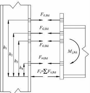
In beam-column connections with extended end-plate, the bending moment resistance is determined by Eq. (1):

,

j Rd r r tr Rd

M



h F

 (1)

where r identifies the bolt lines of the traction zone,

F

tr Rd. is the tension resistant of the bolt line r e

h

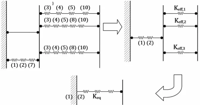
r is the distance between bolts line r and the adopted center of compression, as in Figure 4 .

On the other hand, the rotational stiffness of a connection is obtained from the combination of stiffness values of the components, initially associated in series and later in parallel, as shown in Figure 5 and defined by Eurocode 3 (CEN, 2005) through Eq. (2).

Figure 5: Sequence of calculation of the rotational stiffness of a connection (ROMANO, 2001).

According to Eurocode 3 part 1-8 (CEN, 2005), the rotational stiffness is not considered in the rigidity of the beam component in compression (K7), because this component has an adopted value equal to infinity, due to its rigid-plastic behavior.

To determine the rotational stiffness of a connection, it is first necessary to calculate the effective stiffness of the springs in series associated (

k

ff r,

)

for each both line and then calculate the total equivalent stiffness of the

various lines of both in parallel.

Thus, the Eurocode 3 part 1-8 (CEN, 2005) defines the rotational stiffness of a connection as:

2

1 2

1 1

1

j

eq

Ez

S

k k

k

























(2)

where

E

is the Elastic Modulus of steel,

k

1 and

k

2 are the stiffness values calculated for components 1 and 2, z

is the equivalent lever arm (up to the center of compression),

k

eq is the equivalent stiffness of the components, and

μ is the ratio between initial and secant stiffness.

3 GENETIC ALGORITHM

Genetic algorithms (GAs) are search algorithms based on the natural process, in which individuals that best adapt to the environment would tend to survive. These algorithms are classified as evolutionary algorithms. Genetic algorithms are widely used to solve problems for a given set of elements by finding those elements that best meet the imposed conditions.

The genetic algorithms were initially developed by John Holland in 1965 through a research that initially aimed to study the evolutionary processes, so that the phenomena of adaptation and evolution of the real world were simulated through computational processes (LINDEN, 2012).

Genetic algorithms work with evolutionary principles and genetic theories that can be modeled through computational codes. In general, GAs are flexible and efficient strategies for complex environments, such as the space of solution for the design of a structure (CAMP et al., 1997).

The algorithm begins by arbitrarily defining a population of individuals represented by an analogy with the chromosomes, which represent a set of solution candidates to the problem. The evaluation of the fitness of the individuals of this population is used to generate a new population with better characteristics than those of the previous population. All solution candidates defined in each generation are analyzed to define a numerical quantification in relation to the objective function and the design constraints, which verifies their suitability. According to the suitability of the candidates, operators of reproduction, crossover and mutation are applied to define a new population. This procedure is repeated until it reaches the stop criteria.

4. FORMULATION OF THE PROBLEM

This work aims to develop a methodology to minimize the cost of fabrication of beam-column connections without compromising the mechanical efficiency of the structure, considering the semi-rigid behavior of the connections and using the Components Method of Eurocode 3 (CEN, 2005).

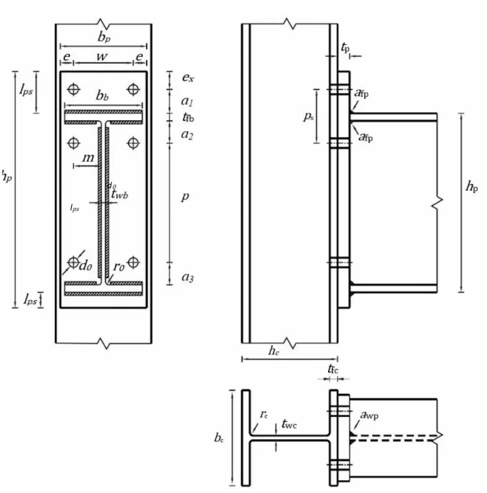
Seven design variables were adopted, as can be seen in Figure 6: the diameter of the bolts (

d

); the thickness of the end-plate (

t

p); the width of the end-plate (

b

p); the horizontal distance between the axis of the bolts and

Figure 6: Geometric parameters of extended end-plate connection (DÍAZ, 2010).

The objective function used in this work considers the total cost of beam-column connections. The total cost comprises the cost of the materials, the cost of labor and the equipment used; it is observed that each component of the connection has a cost different from the other, Eq. (3). This formulation was proposed by Pavlovčič et al.

(2004) and it was also used by Díaz et al. (2012).

, , , ,

US b c t c opm h p s w mf w mc

C

 

C C C



   

C C C C



C

₍₃₎

where,

C

_bis the material cost for the bolt assembly (bolt, nut and two washers),

C

c t, is the cost associated with

the time taken to cut the end-plate,

C

c opm, is the cost of the oxygen–propane mixture used for cutting the

end-plate,

C

h is the hole forming cost,

C

p is the cost of painting the end-plate,

C

s is the cost of the steel for end-plate,

,

w mf

C

is the manufacturing cost for welding the end-plate (including all associated time), and

C

w mc, is the cost of

the welding material consumables (electrodes, wire, etc.).

The equations and costs factors (Table A.1) used to calculate the objective function are shown in Annex A.

d0

The design constraints considered in this work aim to control the minimum allowable values for the bending moment and the rotational stiffness of the connection, according to Eq. (4) and Eq. (5).

, ,

1 0

j Ed j Rd

M

M

 

(4)

,min

_{1 0}

j

j

s

s

 

(5)

where

M

j Ed, is the requesting moment obtained from the optimized steel frame and

S

j min, is the minimum

allowable rotational stiffness value obtained from the optimized steel frame.

In addition, geometric constraints were also considered to verify the lower and higher limits of the design variables,

( )

l

b and

( )

l

b , according to recommendations of Eurocode 3 (CEN, 2005) (Table 1).

Table 1: Lower and upper limits.

Parameter Minimum Value _(mm) Maximum Value _(mm)

p

b

Beam width Column width

e

1,2

d

0 30

x

e

1,2

d

₀ 30

x

p

2,2

d

₀

min



_

200;14 min ,





t t

p fc







_

p

_2,2

_d

₀

min



_

200;14 min ,





t t

_{p fc}







_

w

2,4

d

₀

min



_

200;14 min ,





t t

_{p fc}







_

1

a

y

-

2

a

y

-

3

a

y

-

The values of the holes diameters (Eq. (6)) of the bolts (in mm) are:

1

o

d d

 

_{, if}

_d



₁₂

2

o

d d

 

_{, if}

₁₂

 

_d

₁₂

3

o

d d

 

_{, if}

_d



₁₂

(6)

The minimum distance between the bolts and the beam flange, for that the bolts can be removed without difficulty, is related to the bolt diameter as shown in Eq. (7).

30

y  , if

d



20

35

y  , if

20

 

d

22

40

To use the GA of the MATLAB® optimization toolbox, the constrained optimization problem needs to be transformed into an unrestricted problem, a single equation that considers the simultaneous effect of the objective function and the constraints. For this transformation a penalty function was used based on the level of violation of the constraints. In this case, MATLAB® GA algorithm uses the Lagrangean Augmented method to transform the problem with constraints into an unrestricted problem.

The Augmented Lagrangean Method consists of the combination of the objective function and the nonlinear constraint function, the penalty parameters λi and the slack variables s, as shown in Eq. (8).





2

1 1 1

( , , , ) ( ) log ( ) ( ) ( )

2

m mt mt

i i i i i i m i i p i m i

L x



s p  f x  



S S C x   



ceq x   ceq x (8)

where the parameters



i are known as Lagrange multipliers and are non-negative. The slack parameters

s

i convert the inequality constraints into equalities constraints and are non-negative,



is a positive penalty parameter.

In this way, the algorithm minimizes a sequence of sub problems, each of which approximates the original problem. Each sub problem has a fixed value of λ, s, and ρ. When the sub problem is minimized to a required precision condition and satisfies feasibility conditions, the Lagrangean estimates are updated. Otherwise, the penalty parameter (ρ) is increased. These steps are repeated iteratively until the stop criteria are satisfied.

For the examples presented below, it was used a population of 24 individuals, with 2 of them guaranteed to survive for the next generation. Also, the crossover operator with probability of 0.8 was used.

4.1 Computer modules

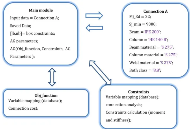
The programming code of this work was developed through the creation of computational modules of analysis and optimization of connections, which were fully developed in the MATLAB® computing environment. In the analysis module, it is used the Component Method, that provides the calculation of the characteristics of resistance and rotational stiffness for the calculation of the design constraints; this module has access through computational interfaces to the database, from where the dimensions and main properties of commercial beams, columns, plates and bolts are obtained.

Initially is established a data entry file with the properties of the frame, in which the connection to be optimized is located, and the requests, for example: the requesting moment, the minimum allowable initial stiffness of the connection, the profiles of beams and columns, the type of analysis and the material of the components. Then, the optimizer module reads the data and stores all the characteristics for the later use of the program.

After reading and storing the input data, the program defines the lateral constraints of the problem (geometric constraints).

Next, the parameters of the AG are defined, such as: population size, number of generations, elitism rate, crossover rate, tolerances of objective function and constraints, etc .; still in the optimizer module, the optimization routine is called.

During the iterative optimization process, the design constraints and the objective function values are calculated. In the constraints module, we first enter the chromosome that was randomly generated by the AG and the profile properties are mapped. In sequence, the tolerance values of the design constraints are read out. With the structure fully defined, the bending moment and the rotational stiffness are calculated. Finally, the constraints are calculated according to Eqs. (4) and (5), necessary steps for the calculation of design constraints.

Figure 7: Computational programming flowchart

5. RESULTS

For validation of the computational tool developed in this work, an application using data available in the literature is presented below. Previously a database was implemented containing geometric properties of commercial profiles, commercial plates and bolts available in manufacturers' catalogs. Access to the database through the analysis and optimization modules is done automatically.

The application considers a plane steel frame of 3 bay and 2 story. Thus, the frame has 4 different connections, according to Figure 8. Previously, this frame was studied by Cabrero and Bayo (2005) and were obtained optimal profiles of beams, columns and minimal values of rotational stiffness and flexural resistance of the connection, as indicated in Table 2. However, this work did not include the optimization of beam-column connections; in 2012, other results for A and C connections were presented by Díaz et al. (2012),

The properties of the materials for these connections are: steel S275, with yield stress



y



275 MPa and

Figure 8: Dimensions and loads for the steel semi-rigid frame optimized in Cabrero and Bayo (2005), the applied loads in kN/m are: wind

q

w=3.80; self-weights

q

sw,0=7.80 and

q

sw,1=6.50; applied

q

il,0=11.20 and

q

il,1=3.20.

The Table 2 shows the optimal profiles of beams, columns and the values of the acting bending moments and the minimum rotational stiffness for frame connections, obtained by Cabrero and Bayo (2005) for this frame.

Table 2: Optimal beams and columns sizes and the stiffness and resistance values for connection.

Connection Beam Column

S

j min,

(kNm/rad)

,

j Ed

M

(kNm)

A IPE200 HE140B 9000 22

B IPE200 HE160B 9000 35

C IPE270 HE140B 16000 40

D IPE270 HE160B 16000 60

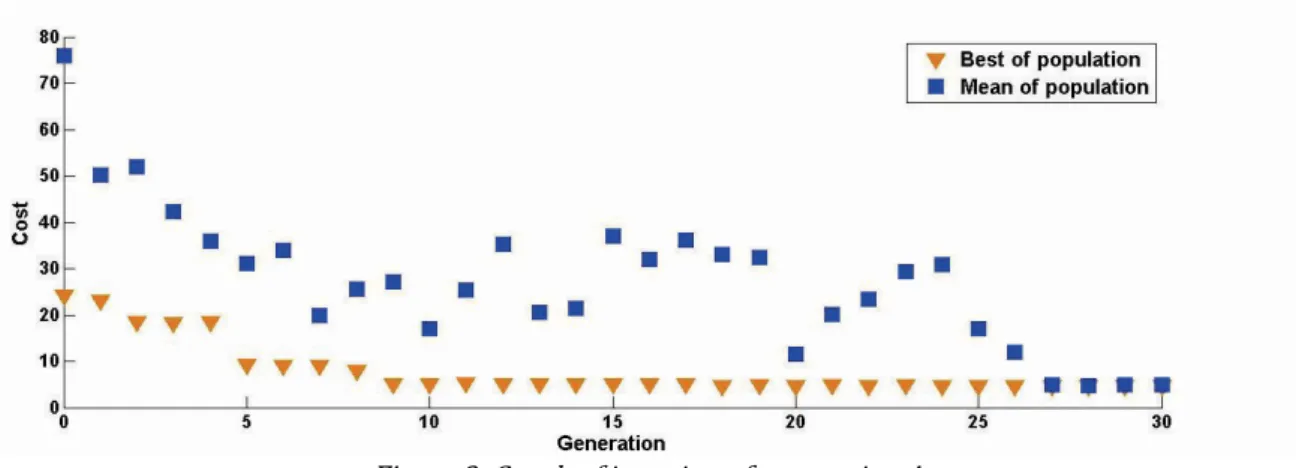
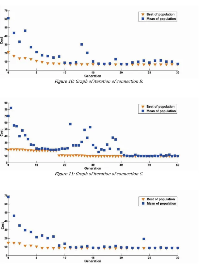
From the optimal configuration shown in Table 2, the optimization of A, B, C and D connections of the frame was performed. The Figures 9 to 12 show the history of the iterations to obtain the minimum cost for each frame connection. The plots show the relationship between the best individual and the average of each generation. All restrictions were met, within the established tolerance. The points outside the iteration curve reflect all the processing of the genetic operators in the formation of the new population of individuals. This type of behavior, very common in GAs, because the GAs have a probabilistic nature.

Figure 10: Graph of iteration of connection B.

Figure 11: Graph of iteration of connection C.

Figure 12: Graph of iteration of connection D.

Table 3: Optimum design variables.

Parameter (mm) Cabrero and Bayo (2005) Díaz et al. (2012) AG (This study)

A B C D A C A B C D

d

20 16 22 22 16 16 12 16 16 16

p

b

140 140 140 140 115 136 101.2 100 135 135

p

h

285 295 345 345 - - 263 266.2 358.5 334.4

p

t

10 12 15 14 12 11 16 9.5 19 12.5

x

p

90 110 70 70 61 61 69.5 82.5 89.3 87.2

w

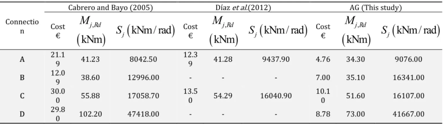
80 80 80 80 - - 45 51.5 75.2 76.5

Table 4 presents the cost (in Euros), the resistant moments and rotational stiffness obtained by Cabrero and Bayo (2005), Díaz et al. (2012) and by this study. To calculate the cost of the connections presented by Cabrero and Bayo (2005), Eq. (3) was used; to obtain the stiffness and the resistant moments, the analysis module of this computational tool was used. The results presented in Table 4 are used to compare and validate the results obtained in this work.

Table 4: Cost, resistant moment and rotational stiffness.

Connectio n

Cabrero and Bayo (2005) Díaz et al.(2012) AG (This study)

Cost €

,

j Rd

M



kNm



S

j

kNm/ rad





Cost €

,

j Rd

M



kNm



S

j

kNm/ rad





Cost €

,

j Rd

M



kNm



S

j

kNm/ rad





A 21.1₉ 41.23 8042.50 12.3₉ 41.28 9437.90 4.76 34.30 9076.00

B 12.0₉ 38.60 12996.00 - - - 7.00 35.10 16341.00

C 30.0₀ 55.88 17058.70 13.5₀ 54.29 16040.90 10.1₀ 51.60 16107.00

D 29.8₀ 102.20 47418.00 - - - 8.78 73.00 41667.00

It is observed that the computational tool presented here obtained good results in comparison with other studies available in the literature. Comparing the costs, this work obtained a reduction of 67% in relation to the results presented by Cabrero and Bayo (2005). In relation to the connections A and C presented by Díaz et al. (2012) the computational tool obtained a reduction of 42%.This high reduction is related to the database, since Díaz et al.

(2012) used bolts with diameters starting 16 mm and this work used a larger database with bolts starting from 12 mm, which gives to AG more possibilities.

The present computational tool was able to increase the efficiency of the connections, so that the values of the resistant moments and the rotational stiffness approximates the minimum admissible value without violating the restrictions.

Figure 16: Details of connection D.

where:

WC_C – Column web in compression failure;

P_F (Mx) – end plate in bending failure (Mx).

CONCLUSION

evaluate the mechanical behavior of the connections and its influence on the optimal component dimensioning. Through the presented example, it was concluded that this computational tool has great potential to obtain optimal dimensions for minimization of cost of connections without violating the normative and constructive constraints.

The computational tool presented here obtained significant improvements in the costs of the connections in relation to the results available in the literature, without compromising the efficiency and safety of the structure. The computational tool obtained a reduction of 67% in the cost of the connections presented by Cabrero and Bayo (2005) and 42% of reduction in the cost of the connections that were presented by Díaz et al. (2012).

In optimization curves it is possible to observe that the mean value decreases, tending to the value of the best solution in each generation, which indicates that the algorithm converged monotonically.

This paper demonstrated, in general, that the optimization of beam-column connections in plane steel frame was successful. The computational tool also automatically determines the optimized profiles from the commercial profiles available in the database.

From the results obtained it is possible to conclude that the optimization model presented in this paper demonstrates to be a robust and effective tool in minimizing the cost of beam-column connections. In addition, the computational environment developed in this work is quite friendly and easy to understand, where the user can easily configure the problem input da and design constraints.

ANNEX A

This annex shows the equations developed by Pavlovčič et al. (2004) to obtain the total cost of a beam-column connection, this annex also shows the cost factor by each of the variable of the objective function.

The calculation of costs (€) and the variables used in the objective function of Eq. (3) were obtained, as shown below.

Material cost for the bolt assembly (bolt, nut and two washers)

,

b b b mt

C n K



2

,

3.076

7.373 4.62

b mt

K



d



d



Cost associated for the time to cut the end-plate





, ,

c t c c c c c ex

C



k f T L T







2

c p p

L



b h



 

2

T

_c

 

0.015

t

_p



0.421 1.43 .5

t

_p



A

.

Cost of the oxygen-propane mixture used for cutting the end-plate





 

, , , , ,

C

_{c opm}



L K M

_{c c mo c o}



K

_{c mp}

M

_{c p}

.6

A

 

2 ,

M

c o



1.645

t

p



56.644

t

p



6.73 .7

A

 

,

M

c p



2.171

t

p



7.87 .8

A

Hole forming cost







/ ,



h h h ep ex d h ex

C k n t t V T

ep p fc

t

 

t t

2

0 0

0.763

5.720

20.96

d

V



d



d







,



2

p p p p pain p mt p

C



b h

k T



k M

Cost of the steel for the end-plate

s s ep s

C kV





ep p p p

V b h t



Manufacturing cost for welding the end-plate













, , , ,

Cw mf Kw f Tw w afLf Tw aw wL Tw ex .15 A









L

_f



2

b

_b



b

_b



2

r t

_b



_wb

.16

A









L

w



2

h

b



2

r t

b



fb

.17

A





2 ,

T

_{w af}



9.03

a

_f



4.68

a

_f



0.82 .18

A





2 ,

T

_{w aw}



9.03

a

_w



4.68

a

_w



0.82 .19

A

Cost of the welding material consumables (electrodes, wire, etc.)









, , , , , ,

C

_{w mc}



k

_{w mt}

M

_{w mc af}

L

_f



M

_{w mc aw w}

L

.20

A





2 , ,

M

w mc af



0.66

a

f



0.18

a

f



0.10 .21

A





2 , ,

M

w mc aw



0.66

a

w



0.18

a

w



0.10 .22

A

Table A.1: Summary of the cost factor used in the objective function.

Parameter Minimum Value _(mm) Maximum Value (mm)

s



7820 kg/m3 _{Steel mass density}

c

f

1.03 - Cutting factor that increases labor

w

f

1.4 - Welding factor that increases labor

,

b mt

k

Eq.(A.2) €/bolt Unit cost of bolt

c

k

0.307 €/min Unit cost for cutting

, ,

c m o

k

0.0016 €/l Unit cost of oxygen

, ,

c m p

k

0.0020 €/l Unit cost of propane

h

k

0.323 €/min Unit cost for hole forming

p

k

0.43 €/min Unit cost for painting

,

p mt

k

3.8 €/l Unit cost of paint

s

k

0.4 €/kg Unit cost of steel

w

k

0.123 €/min Unit cost for welding

,

wmt

k

1.4 €/kg Unit cost of weld

c

L

Eq.(A.4) M Cutting length

f

L

Eq.(A.16) M Length of weld between beam flange and end-plate of thickness

a

f

w

L

Eq.(A.17) M Length of weld between beam web and end-plate of thickness

a

_w

,

c o

M

Eq.(A.7) l/m Material consumption of oxygen

,

c p

M

Eq.(A.8) l/m Material consumption of propane

p

M

0.15 l/m2 _{Paint consumption}

, ,

w mc af

M

Eq.(A.21) Kg/m Material consumption for a weld of length

L

f and thickness

a

f

, ,

w mc aw

M

Eq.(A.22) Kg/m _{Material consumption for a weld of length}

L

_{w and thickness}

a

_w

b

n

6 Bolt Number of bolts

h

n

6 Hole Number of holes

c

T

Eq.(A.5) min/m Cutting time

,

c ex

T

2.0 Min Additional cutting time

ex

t

1.4 Cm Additional drilling path

,

h ex

T

11.9 Min Additional hole forming time

ep

t

Eq.(A.10) Cm Thickness of drilled plate

pain

Table A.1: Continuation.

Parameter Minimum Value _(mm) Maximum Value (mm)

,

w af

T

Eq.(A.18) min/m Welding operational time for a weld of length

L

f and thickness

a

f

,

waw

T

Eq.(A.19) min/m Welding operational time for a weld of length

L

_wand thickness

a

_w

,

w ex

T

0.3 Min Additional welding time

d

V

Eq.(A.11) cm/min Drilling speed of progression

ep

V

Eq.(A.14) m3 _{Volume of end-plate}

Where

a

f,

a

_w,

d

₀,

d

,

t

p are in cm.

REFERENCES

ABNT – Brazilian Association of Technical Standards, (2008). Structural Steel Design and Mixed Steel and Concrete Structure of Buildings: NBR 8800. 237 p., Rio de Janeiro.

Cabrero J.M., Bayo E., (2005). Development of Practical Design Methods for Steel Structures with Semirigid Connections. Eng Struct, 27:1125–1137.

Camp, C. V; Pezeshk, S.; Cao, G., (1997). Design of Framed Structures Using a Genetic Algorithm. Advances in Structural Optimization, p. 19-30, Reston.

Castro, R. A., (2006). Computational Modeling of Semi-rigid Connections and its Influence on Nonlinear Dynamic Response of Steel Frame. Master’s dissertation. Postgraduate Program in Civil Engineering (PGECIV). State University of Rio de Janeiro, Rio de Janeiro.

CEN - European Committee for Standardization (2005). Design of steel structure. Part 1.8: design of joints, EN 1993-1-8, Eurocode 3. Brussels. 138 p.

Degertekin, S.O.; Hayalioglu, M.S. (2010). Harmony search algorithm for minimum cost design of steel frames with semi-rigid connections and column bases. Structural Multidisciplinary Optimization, 42: 755-768.

Díaz, C., (2010). Optimal Design Semirigids Connections by Numerical Simulation and Kriging Models. Doctoral thesis in Civil Engineering, Cartagena Polytechnic University, Cartagena.

Díaz C., Victoria M, Martí P, Querin OM., (2012). Optimum Design of Semi-rigid Connections Using Metamodels. Journal of Constructional Steel Research, 78:97-106.

Faella, C; Piluso, V e Rizzano, G., (2000). Structural Steel Semi-rigid Connections: Theory, Design and Software. 536 p., CRC Publisher, Boca Raton - Florida.

Falcón, G.A.S, Montrull, P.M. (2014). Optimum Dimensioning of semi-rigid connections of Steel frame - “Auxiliary Frame” Model. XXXV Iberian Latin American Congress on Computational Methods in Engineering, 22 p.

GOE – Structural Optimization Group (2010). CalcUS_MC. Program in MATLAB for calculation of resistance and Stiffness of semi-rigid connections by the method of components. Cartagena Polytechnic University (UPCT), Cartagena.

Hayalioglu, M. S., Degertekin, S. O., (2005). Minimum Cost Design of Steel Frames with Semi-rigid Connections and Column Bases via Genetic Optimization. Computres & Structures, 83 (2005) 1849–1863.

Linden, R., (2012). Genetic Algorithms. 496 p., Modern Science, Rio de Janeiro.

Pavlovčič L, Krajnc A, Beg D, (2004). Cost Function Analysis in the Structural Optimization of Steel Frames. Struct Multi Optim, 28:286–95.

Romano, V.P., (2001). Design of Beam-Column Connections with Top Plate: Eurocode Model 3. Master’s dissertation, Postgraduate Program in Civil Engineering, Federal University of Ouro Preto, Ouro Preto.

Simões, L. M. C. (1996). Optimization of Frames with Semi-rigid Connections. Computres & Structures, v. 60, n. 4, p. 531-539.