Macro-financial linkages between emergent and sustainable economies in a context of the European sovereign debt crisis

Publication Date: Aug. 25, 2018 DOI: 10.14738/abr.68.4981. Ferreira, N. B. (2018). Macro-financial linkages between emergent and sustainable economies in a context of the European sovereign debt crisis. Archives of Business Research, 6(8), 109-121.

Macro-financial linkages between emergent and sustainable

economies in a context of the European sovereign debt crisis

The aim of the study is to identify the international economic linkages between European emergent countries and different economies under the European sovereign debt crisis from the 1990s through 2015. More precisely, we compared the worst-performing European economies with more economically sustainable economies (such France, Germany, the United Kingdom and Norway). Switzerland, China, Japan and the United States were also included to evaluate the external impacts on the European Union. To examine the increasing macro-financial linkages, their interactions were included in the Global VAR model. Credit variables and oil were used to analyse international transmission of the Euro area along with the US, China, Japan and Switzerland credit and aggregate demand shocks. The model was set up with quarterly data from a sample of 11 countries, and the followed global economic variables that included: Real GDP, inflation, real equity prices, real exchange rates, government bonds (10 year), interest rates (3 month) and the price of oil. The results showed that the US influence was contracted since all macroeconomic variables did not react significantly with the oil and US long-term interest rate shocks.

Keywords: GVAR analysis, national and regional shocks, impulse response analysis, trade

weights

INTRODUCTION

The world economies are closely interlinked, via complex diffusion networks, which are difficult to model empirically. Bilateral relationships between economies are a necessary condition for sharing scarce resources (such as oil and other commodities), political and technological developments, cross-border trade in financial assets, as well as trade in goods and services and labour. Even after allowing for such factors, there might still be residual interdependencies due to unobserved interactions and spillover effects not taken properly into account by using the common channels of interactions. The GVAR, a VAR based model of the global economy, offers a solution to the so-called "curse of dimensionality." That is, the existence of too many parameters to be estimated on the available observations ([1] [2] [3] [4]). In summary, the GVAR can be viewed as a two-step procedure. In the first step, small-scale country-specific models are estimated conditionally based on the rest of the world. In the second step, individual country VAR models are stacked and solved simultaneously as one large global VAR model. The solution can be used for shock scenario analysis and forecasting as is usually done with standard low-dimensional VAR models. In this context, it is usual to present three main models that use common factors (e.g. small-scale factor-augmented VARs, Bayesian VARs and the global VARs). Individual units need not necessarily be countries, but could be regions, industries, goods categories, banks, municipalities, or sectors of a given economy, just to mention a few notable examples [5]. Mixed cross-section GVAR models, for instance, linking country data with firm-level data, have also been considered in the literature ([6] [7] [8] [9]).

In financial markets for the Euro area we have a "typical market" (or single market) which is the large primary development toward full economic integration. After the Lehman Brothers

debt crisis, different regional co-movements of real outputs and other macroeconomic variables drove external shocks or self-sustaining development in the world, and the impact regarding economic blocks integration has not yet been rigorously demonstrated. In this context, the relative importance of regional shocks originating from China and US needs to be considered when establishing a new pattern of world market integration after the Lehman debt crisis. Thus, the GVAR model was developed for the purpose of capturing spillovers in multi-country analyses, where restrictions arise as a result of the weights imposed on foreign variables, as well as from the homogeneity of each foreign factor on the long-run parameters of the corresponding VAR [10]. The past decade have witnessed several debt crises we are also interested in indagating if the predominant role of US remains valid. The paper is structured as follows: Section 1 introduces our empirical framework (the GVAR model); Section 2 reviews the scientific literature; Section 3 presents the GVAR methodology; Section 4 describes the data; Section 5 outlines the results. After the results were calculated, we obtained the impulse function response analysis, which constitutes Section 6; and Section 7 provides the conclusion. STATE OF THE ART

Since the introduction of the GVAR model by Pesaran et al. [11] there have been several applications of the GVAR approach in academic literature, especially over the last decade (e.g., the GVAR Handbook, edited by di Mauro and Pesaran [12], which provides an interesting collection of some GVAR empirical applications). This methodology has also found acceptance in policy institutions, including the International Monetary Fund (IMF) and European Central Bank (ECB), where this is one of the main methods used to distinguish interlinkage across different countries ([7] [8] [9]). The first attempt at a theoretical defence of the GVAR approach was provided by Dées et al. [13] (DdPS), who derived the VAR model augmented by the vector of the star variables and their lagged values as an approximation to a global VAR. The GVAR approach was initially established as a result of the 1997 Asian financial crisis to compute the effects of macroeconomic developments on the losses of major financial organisations. It was clear then that all major banks are highly exposed to systemic risk from adverse global or regional shocks, but quantifying these effects required a coherent global macroeconomic model [14].

Dreger and Wolters [15] investigated the implications of an increase in liquidity in the years preceding the global financial crises on the formation of price bubbles in asset markets. The implications of liquidity shocks and their transmission were also investigated in Chudik and Fratzscher [16]. In addition to liquidity shocks, Chudik and Fratzscher [16] identified risk shocks, and found that while liquidity shocks have had a more severe impact on advanced economies during the recent global financial crisis, it was mainly the decline in risk appetite that affected emerging market economies. Bussière, Chudik and Mehl [17] found that the reactions of real effective exchange rates in Euro countries to a global risk aversion shock after the creation of euro have become similar to those in Italy, Portugal and Spain before the European monetary union, i.e., of economies in the Euro areas' periphery. Some other empirical GVAR papers that focused on modelling various types of risk (e.g. [18]) analysed interactions between banking sector risk, sovereign risk, corporate sector risk, real economic activity, and credit growth for 15 European countries and the US. In addition, Dovern and van Roye [19] used a GVAR to study the international transmission of financial stress and its effects on economic activity, whereas Feldkircher [20] assessed the spatial propagation and

Copyright © Society for Science and Education, United Kingdom 111 the time profile of foreign shocks to the region and Gross and Kok [21] used GVAR specification to investigate contagion among sovereigns and banks.

Cesa-Bianchi, Pesaran, and Rebucci [22] explored the interrelation between volatility in financial markets on macroeconomic dynamics, who extended the GVAR model of DdPS by a volatility module. Finally, Feldkircher and Huber [23] analysed international spillovers of expansionary US aggregate demand and supply shocks and of a contractionary US monetary policy shock.

GVAR METHODOLOGY

The analysis was performed using the global vector autoregressive (GVAR) methodology, originally developed by Pesaran et al. [11] and further developed by Dées et al. [13]. The GVAR approach is a relatively novel empirical methodology used to examine a global macroeconomic environment. This methodology combines time series, panel data and factor analysis techniques. Pesaran, Schuermann and Smith [24] provided an overview of this modelling technique. di Mauro and Pesaran [12] offered a board-based collection of the more relevant studies using GVAR during the last decade. The GVAR model is based on the following assumptions: I. There are N+1 countries or regions. II. The country-specific variables are related to global economic variables. Global economic variables include three groups: 1) Country-specific weighted averages of foreign variables 2) Deterministic variables, such as time trends 3) Global (weakly) exogenous variables, such as oil prices

There are country-specific variables xit. There are (k k_i× _i*) foreign-specific variables specific to

the ith _{country. It was considered N+1 countries in the global economy, by i=0,1,…, N. Except for}

the US, which was labelled as zero and taken to be the reference country; all other N countries were modelled as small open economies. For each country, we considered two types of variables: (1) domestic variables, and (2) foreign variables. Each economy was linked to the others by the foreign variables and calculated as weighted averages of the corresponding country-specific variables, as well as the global (weakly) exogenous variables, such as oil prices and the deterministic variables, such as time trends.

This set of individual VARX* models was used to build the GVAR framework. Following Pesaran

et al. [11] and Dees et al. [12], a VARX*(pi, qi) model for the ith _{country relates a ki x 1 vector of}

domestic macroeconomic variables (treated as endogenous), xit, to a ki*

x 1 vector of country-specific foreign variables (taken to be weakly exogenous), xit*:

Φ₃ = 4, 6₃ 7₃₈ = 9_3%+ 9₃₍: + Λ₃ 4, <₃ 7₃₈∗ _{+ >}

38, (1)

For t=1,2,…,T, where ai0 and ai1 are kix one vectors of fixed intercepts and coefficients on the

deterministic time trends, respectively. Uit is a kix one vector of country-specific shocks, which

were assumed were serially uncorrelated with zero mean and a non-singular covariance matrix, ∑ii, namely uit~i.i.d.(0,∑ii). For algebraic simplicity, observed global factors in the

country-specific VARX* models abstracted. Furthermore, Φ₃ 4, 6₃ = ? − AB Φ₃43

3C( and

Λ₃ 4, <₃ = ? − DB Λ₃43

3C% were the matrix lag polynomial of the coefficients associated with the

domestic and foreign variables, respectively. As the lag orders for these variables, pi and qi,

were selected on a country-by-country basis, we were explicitly allowing for Φ₃ 4, 6₃ and Λ₃ 4, <₃ to differ across countries.

The country-specific foreign variables were constructed as cross-sectional averages of the domestic variables using data on, for example, bilateral trade as the weights, wij: 7₃₈∗ _{= E} 3F7F8, G FC% (2) Where j=0,1,…,N, wij=0, and G_FC%E_3F = 1.

Although estimations were calculated on a country-by-country basis, the GVAR model was solved for the world as a whole, taking account of the fact that all variables were endogenous to the system as a whole. After estimating each country VARX*(pi, qi) model separately, all the k= G J₃ 3C% endogenous variables, collected in the k x 1 vector 78= 7´%8L , 7(8L , … , 7G8L L, needed to be solved simultaneously using the link matrix defined in terms of the country-specific weights. To see this, the VARX* model in equation (1) can be more compactly written as: N₃ = 4, 6₃, <₃ O₃₈ = P₃₈, (3) for i=0,1,…,N, where N₃ = 4, 6₃, <₃ = Φ₃ 4, 6₃ − Λ₃ 4, <₃ , O₃₈ = 7_´38L _{, 7} 38L∗ ′, P₃₈ = 9_3%, 9₃₍: + >₃₈. (4) Note that given equation (2) can be written as: O₃₈ = R₃7₈, (5)

Where Wi = (Wi0, Wi1, …, WiN), with Wii = 0, is the (ki+k*i) x k weight matrix for country i defined

by the country-specific weights, wij. Using (5), (3) can be written as:

N₃ = 4, 6 R₃7₈ = P₃₈, (6)

N₃ = 4, 6 is constructed from N₃ = 4, 6₃, <₃ by setting p=max(p0,p1,…pN, q0,q1,…,qN) and

augmenting the p-pi or q-qi additional terms in the power of the lag operator by zeros. Stacking

equation (6), the Global VAR(p) model was obtained in domestic variables only: S 4, 6 7₈= P₈, (7) Where S 4, 6 = N%(4, 6)R% N₍(4, 6)R₍ .. . N_G(4, 6)R_G , P₈ = P_%8 P₍₈ .. . PG8 . (8) For an early illustration of the solution GVAR model, using a VARX*(1,1) model, see Pesaran et al. [11], and for an extensive survey of the latest developments in GVAR modelling, both the theoretical foundations of the approach and its numerous empirical applications, see Chudik and Pesaran [2]. The GVAR(p) model in equation (7) can be solved recursively and used for some purposes, such as forecasting or impulse response analysis.

Copyright © Society for Science and Education, United Kingdom 113 Chudik, Alexander and Pesaran [25] extended the GVAR methodology to a case in which common variables were added to the conditional country models (either as observed global factors or as dominant variables). In such circumstances, equation (1) should be augmented by a vector of dominant variables, ωt, and its lag values: Φ3 4, 63 738 = 93%+ 93(: + Λ3 4, <3 738∗ + Υ3 4, W3 X8+ >38, (9) Υ3 4, W3 = Y3C%B Υ343 is the matrix lag polynomial of the coefficients associated with the common

variables. Here, ωt can be treated (and tested) as weakly exogenous for the purpose of

estimation. The marginal model for the dominant variables can be estimated with or without feedback effects from xt. To allow for feedback effects from the variables in the GVAR model to the dominant variables via cross-section averages, we defined the following model for ωt: X₈ = Φ_Z[X_3,8\[ + Λ_Z[7_3,8\[∗ _{+ ]} Z8 A^ [C( A^ [C( (10) It should be noted that contemporaneous values of star variables (* superscript) do not feature in the previous equation, and ωt are 'causal.' Conditional and marginal models can be combined and solved as a complete GVAR model as explained earlier. Data and model specification

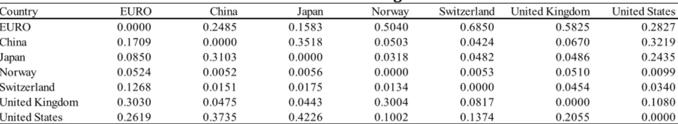
In this paper, the GVAR model contained 11 countries from different regions of the world. Table 1 presents countries and regions included in the model. The estimation was made using five countries (Portugal, Ireland, Greece, France and Germany) grouped together in the Euro area and treated as a single economy, while the remaining six were modelled individually. The model estimated for 22 years (January 1993 through December 2015). Foreign variables are denoted by a * it x vector and were constructed as weighted averages with country-specific weights used to specify the pattern of economic relations among the countries of interest. The country-specific foreign variables were built using fixed trade weights based on the average trade flows computed over 20 years, i.e., 1993–2013, and are defined as follows: _<sub>`a</sub>∗ <sub>= b</sub> `c_`a, d cCe fg`a ∗ _{= b} `cfg`a, d cCe hih`a ∗ <sub>= b</sub> `chih`a , d cCe

Where wit, the weights, are the share of country j in the trade of country i, such that wit=0 and

b_`c= j

d

cCe . The motivation behind choosing the trade weights was to accommodate the

effects of external shocks that could pass through output in all countries via trade channels.

Table 1. Trade weights

Country EURO China Japan Norway Switzerland United Kingdom United States

EURO 0.0000 0.2485 0.1583 0.5040 0.6850 0.5825 0.2827 China 0.1709 0.0000 0.3518 0.0503 0.0424 0.0670 0.3219 Japan 0.0850 0.3103 0.0000 0.0318 0.0482 0.0486 0.2435 Norway 0.0524 0.0052 0.0056 0.0000 0.0053 0.0510 0.0099 Switzerland 0.1268 0.0151 0.0175 0.0134 0.0000 0.0454 0.0340 United Kingdom 0.3030 0.0475 0.0443 0.3004 0.0817 0.0000 0.1080 United States 0.2619 0.3735 0.4226 0.1002 0.1374 0.2055 0.0000 The set of country-specific foreign variables represents the dynamics of the global economic variables, The set of country-specific foreign variables represents the dynamics of the global economic variables, which were assumed to impact and shape macroeconomic variables. In the case of the US economy, domestic and foreign variables were treated differently because the US

was treated as a reference country. The US model was linked to the world through the assumption that exchange rates were determined in the remaining country-specific models. Therefore, we have the following domestic and foreign variables for the US model:

xit = (yit, dpit, eqit, epit, rit, irit) and x*it = (y*it, dp*it, eq*it, r*it, ir*it, poilt)

where yit is the log real output, exit is the log real exports, imit is the log real imports, rerit is the

log real effective exchange rates, dpit is the log of the rate of inflation and poilt is the log of the

nominal spot price of oil. Given the importance of the US economy in the global economy, we included the price of oil as an endogenous variable. We considered the set of real exchange rates as weakly exogenous for the US model, while the real exchange rates were treated as an endogenous variable and the price of oil preserved as an exogenous variable in the models for all other countries. The economies modelled by GVAR methodology interact through three interrelated channels: 1. Domestic variables xit depend contemporaneously on foreign variables x_it* and on their

lagged values.

2. Dependence of the country-specific (domestic) variables on common global exogenous variables.

3. Shocks in country i depend contemporaneously on shocks in country j, captured by the covariance matrix ij , where ij=cov ( ,ar u u_{it jt})=E u u( ,_{it jt}) for i j.

EMPIRICAL RESULTS ANS DISCUSSION

Although the GVAR model can be estimated using stationary and non-stationary variables, the perfect evidence about the order of integration is crucial and plays an important role. The assumption allows distinguishing short- and long-run relations and interpreting that long-run as co-integrating. The I (first) assumption cannot be rejected for the majority of the endogenous and exogenous variable. The results of unit root tests were not reported in this text, but they are available upon request. We proceeded with the estimation of the VAR relationships (i.e., coefficients of individual country models), which revealed stability over time.

In the following analysis particular attention was given to testing for the adjustment coefficients for the error-correction models, and the solved cointegrating vectors normalised on the real effective exchange rate presented in Tables 2 and 3.

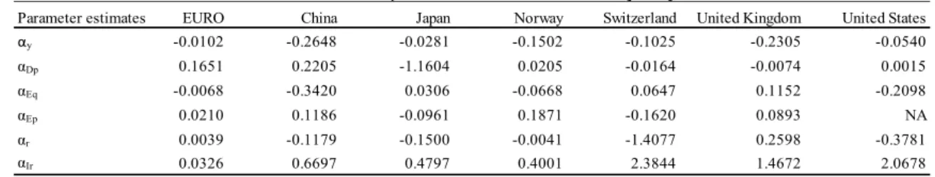
Table 2. Adjustment coefficients (CVI)

Parameter estimates EURO China Japan Norway Switzerland United Kingdom United States

αy -0.0102 -0.2648 -0.0281 -0.1502 -0.1025 -0.2305 -0.0540 αDp 0.1651 0.2205 -1.1604 0.0205 -0.0164 -0.0074 0.0015 αEq -0.0068 -0.3420 0.0306 -0.0668 0.0647 0.1152 -0.2098 αEp 0.0210 0.1186 -0.0961 0.1871 -0.1620 0.0893 NA αr 0.0039 -0.1179 -0.1500 -0.0041 -1.4077 0.2598 -0.3781 αIr 0.0326 0.6697 0.4797 0.4001 2.3844 1.4672 2.0678

Copyright © Society for Science and Education, United Kingdom 115

Table 3. Estimated coefficients of the solved cointegrating vectors

Parameter estimates EURO China Japan Norway Switzerland United Kingdom United States

Trend 0.0000 -0.0024 -0.0399 -0.0053 -0.0042 0.0024 -0.0070 βy 0.0000 1.0000 1.0000 1.0000 1.0000 1.0000 1.0000 βDp -1.0000 0.0000 0.0000 0.0000 0.0000 0.0000 0.0000 βEq 0.0000 0.1820 0.3131 0.0000 0.0000 0.0000 -0.0762 βEp 0.0000 1.0302 -4.2156 -0.6028 1.3861 -1.6455 NA βr 1.0000 0.1224 3.5082 -0.7387 0.0765 0.2246 0.6451 βIr 0.0000 -0.2082 -0.2322 0.4053 0.0091 -0.0135 -0.1397 βys 0.0000 -0.3387 0.2009 -2.4428 0.8013 0.6372 0.1168 βDps 0.0000 0.0321 -2.1817 -0.1160 0.1331 0.0904 -0.0038 βEqs 0.0000 0.0954 -0.1286 0.8830 0.0076 -0.1315 NA βEps NA NA NA NA NA NA -0.1961 βrs 0.0000 -0.1296 2.4221 -0.6692 0.0609 -0.2988 NA βIrs 0.0000 -0.0471 -0.3315 -0.0717 -0.1255 0.0656 NA βpoil 0.0000 0.0250 1.3390 0.0324 -0.1616 -0.1163 0.0918

The market models were tested individually for the number of cointegrating relations occurring in each model. The Johansen test was applied in all cases) Since the VARX*(pi, qi) models include foreign variables as exogenous, an assumption was that domestic variables have no impact on their foreign equivalents.

The empirical cross-country correlations for the data set are summarised in Table 4. This table reports such correlation coefficients computed as averages of the correlation coefficients between the levels, first differences and residuals of each equation (variable) with all other country/region equations. Table 4. Average pairwise cross-section correlations of the residuals of each VECMX Country Levels First Differences VECMX Residuals Levels First Differences VECMX Residuals EURO 0.6681 0.5193 -0.1907 -0.0922 0.1557 -0.0083 China 0.3780 0.0871 -0.1580 -0.1902 0.0851 -0.0914 Japan 0.6283 0.2493 0.0064 0.0423 0.1303 0.0461 Norway 0.3785 0.4269 -0.0632 0.3723 0.1733 0.0901 Switzerland 0.5857 0.3983 -0.0779 0.3816 0.2652 0.1167 United Kingdom 0.3029 0.4947 -0.0879 0.3852 0.2132 0.0594 United States 0.4791 0.2419 -0.0524 0.3910 0.2624 0.0860 Country Levels First Differences VECMX Residuals Levels First Differences VECMX Residuals EURO 0.7393 0.5845 -0.1186 0.2479 0.0800 0.1530 China 0.6092 0.2074 -0.1239 0.1687 0.0467 0.0819 Japan -0.0885 -0.0110 -0.1511 -0.4570 -0.1058 -0.0264 Norway 0.6567 0.5255 0.0048 0.2138 0.1131 0.1071 Switzerland 0.7127 0.5019 -0.0406 0.2223 0.1068 0.1015 United Kingdom 0.6799 0.6107 0.0362 -0.3129 -0.3090 0.0782 United States 0.6718 0.5603 0.0531 NA NA NA Country Levels First Differences VECMX Residuals Levels First Differences VECMX Residuals EURO 0.5747 0.2907 0.0234 0.6529 0.1686 -0.0523 China 0.3094 0.0344 -0.0116 0.5109 0.1627 0.0250 Japan -0.6317 -0.1084 -0.0414 0.4588 0.1386 0.0001 Norway 0.5449 0.2691 0.0438 0.6729 0.2651 0.0632 Switzerland 0.4978 -0.0419 0.0111 0.6743 0.1552 0.0235 United Kingdom 0.5754 0.3282 0.0238 0.7175 0.2974 -0.0073 United States 0.5338 0.3177 0.1429 0.7064 0.1978 0.0491

Real GDP (y) Inflation (Dp)

Real Equity Prices (Eq) Real Exchange Rate (Ep)

Government Bond 10y (r) Interest rate (Ir)

A two-tailed t-test rejected the hypothesis that these coefficients were significantly different from zero at the conventional level. The highest correlation averages on levels, among the six analysed variables, were 0.49 (real GDP), 0.57 (real equity prices) and 0.63 (interest rate - 3M). The findings suggest a significant co-movement for those variables and less synchronisation for the remaining.

There are still noticeable correlations in the first difference, as the average correlations range between 43% (real equity prices) and 16% (government bond 10 year), except for the real exchange rate variable. Regarding the residuals coefficients, the low correlations obtained — one of the main conditions for a well-functioning VAR model — confirmed the fitness of the model.

After having individually estimated each country-VARX* model (Table 5), the assumption of weak exogeneity of the foreign variables of each country using the weak exogeneity tests, was tested. In this way, it tested the joint significance of the estimated error-correction terms for the country-specific foreign variables and oil prices.

One of the main assumptions of the GVAR model was weak exogeneity, i.e., that there is no long-run imposing effect from country-specific domestic to foreign variables. This implies that if we assumed foreign country-specific prices to be weakly exogenous means that all countries are assumed to be small economies in the rest of the world. To check the assumption, we performed a formal test for all country-specific foreign variables, as well as for the global variables. The null hypothesis of weak exogeneity was rejected for all variables in all models. (NA stands for non-available data.)

The estimation of the cointegrating VARX models provided the opportunity to examine the feedback of foreign-specific variables on their domestic counterparts, as derived by the coefficients estimates related to contemporaneous foreign variables in differences, which are viewed as impact elasticities. Table 5. Test for weak exogeneity at the 5% significance level 5% CV d.f. EURO 0.7489 4.8063 0.9246 NA 1.0563 0.7049 1.0685 3.1221 (2,73) China 0.3853 0.0370 2.8013 NA 1.2272 1.7448 0.1788 3.1221 (2,73) Japan 1.7952 0.8632 1.4496 NA 1.7274 0.5816 1.8789 3.1221 (2,73) Norway 1.2859 0.8632 0.6058 NA 0.9718 1.1631 0.8736 2.7318 (3,72) Switzerland 1.1477 0.3243 0.1439 NA 0.1705 1.4545 0.5403 2.7318 (3,72) United Kingdom 0.0892 0.8238 0.3123 NA 0.6529 3.4466 1.2783 2.7318 (3,72) United States 1.0878 3.0191 NA 0.1508 NA NA 0.9756 3.1154 (2,77) Irs poil F-statistic

Country ys Dps Eqs Eps rs

Impact elasticities measured the contemporaneous variation of a domestic variable due to a 1% change in its corresponding foreign-specific counterpart, and they were particularly useful in the GVAR framework in identifying general co-movements among variables across countries. Table 6 shows the impact elasticities with the corresponding t-ratios, computed based on White's heteroscedasticity-consistent variance estimator.

Dées et al. [13] asserted these estimates could be interpreted as impact elasticities between domestic and foreign variables. Most of these elasticities were significant and had a positive sign, as expected. They are particularly informative as regards the international linkages between the domestic and foreign variables. Focusing on the Euro area, we could see that a 1% change in real foreign output in a given quarter led to an increase of 0.5% in Euro area real output within the same quarter. Similar foreign output elasticities were obtained across the different regions.

Another interesting feature of the results is the very weak linkages that seem to exist across short-term interest rates, (Sweden being an exception) and the significant relationships across

Copyright © Society for Science and Education, United Kingdom 117 long-term rates. This fact clearly shows a much stronger relationship between bond markets than between monetary policy reactions. A closer inspection of the elasticities values in Table 6 show very high elasticities for Eq. A 1% change in the oil price in the Euro zone caused the Eq. variables to increase 1.34%, a very strong, significant response.

From this table we can see that the impact elasticities related to foreign real GDP are positive and statistically significant in all cases, highlighting a remarkable degree of synchronization in the output dynamics across economies. This suggests that when countries suffer from domestic-generated GDP growth pressures, their dynamics are dependent on the internal developments of foreign countries. All estimate values lie between zero and one, in particular, the lowest value obtained was for China (0.0674), while the highest are associated with Euro (1.8403) and Switzerland (1.2845). Table 6. Contemporaneous effects of foreign variables on their domestic counterparts EURO 1.8403 -0.4217 1.3472 0.1212 0.2596 [13.5380] [-0.6068] [12.0688] [0.6582] [2.2071] China 0.0674 0.0004 0.3500 -0.1764 -0.0195 [0.2090] [0.0741] [1.7320] [-0.8457] [-0.9153] Japan 0.0455 -1.6082 -0.2840 -0.4799 0.2106 [0.9305] [-1.5103] [-1.0626] [-2.1161] [0.6997] Norway 0.8328 0.0017 1.0289 1.2986 0.1012 [5.9822] [0.3667] [9.7762] [10.7519] [1.8852] Switzerland 1.2845 -0.0009 0.7478 -1.0650 0.7377 [11.8672] [-0.4721] [12.3953] [-1.9516] [1.9199] United Kingdom 1.0485 0.0006 0.8255 0.5963 0.1420 [10.5136] [0.2396] [19.5993] [9.5304] [2.9636] United States 0.0436 0.0037 NA NA NA [1.1283] [1.9034] NA NA NA Ir Country y Dp Eq r

Impact elasticities greater than one reveal an overreaction of the headline inflation in these countries on the increase in GDP of their main trading partners. It also appears that low elasticities are associated with large countries, while the opposite holds for small countries. This is compatible with the general finding that the transmission channel of GDP works mostly unidirectional from large to small countries. This finding was also evidenced by Galesi and Lombardi [26].

Impulse response functions

Impulse response functions provided counterfactual answers to questions concerning the effects of a particular shock in a given economy, or the effects of a combined shock involving linear combinations of shocks across two or more economies. The effects of the shocks can also be computed either on a particular variable in the global economy, or on a combination of variables. The GIRFS are defined as:

1 (y , , ) n j u t t j j u F G s GIRF u n s s

= , where s_j denotes a binary shock indicator vector, n is the shock horizon,

u

is the corresponding variance covariance matrix of the GVAR and _{F G H=} 1 _{. The dynamic analysis was carried out on the levels of the}

variables, which implies that the effects of a given shock are typically permanent. The propagation of five different macroeconomic shocks, in terms of a positive standard error (s.e.) shock to all markets in relation to y – log real output; Dp - log of rate of inflation; r – 10 years

government Bond rates; Ir - interest rates 3 months, was also studied.

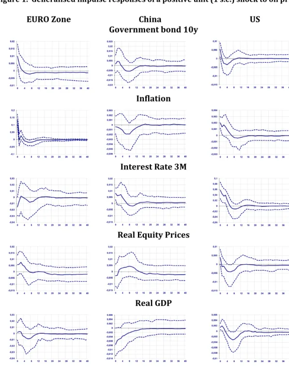
Figure 1. Generalised impulse responses of a positive unit (1 s.e.) shock to oil prices. EURO Zone China US Government bond 10y Inflation Interest Rate 3M Real Equity Prices Real GDP

Copyright © Society for Science and Education, United Kingdom 119 Figure 2. Generalised impulse responses of a positive unit (1 s.e.) shock to Government bond 10Y (US). EURO Zone China US Government bond 10y Inflation Interest Rate 3M Real Equity Prices Real GDP FINAL REMARKS

The shocks were divided into two categories: One were real shocks (e.g. macroeconomic variable shock); the second included the US long-term interest rate shock for each macroeconomic variable. The main goal in taking this approach was to see how the impact of these shocks originating in particular markets were felt and transmitted across other countries and regions. Initially, we looked at the response of the global economy to a one standard error positive to oil price [Figure 1]. As expected, oil importers, such as the US, the Euro area, Switzerland, the UK and Japan were negatively affected by the rise in oil prices. This effect was observed with more evidence in the 10 year government bond and in the inflation rate, which revealed the co-movement between oil price and these two variables. China was the most affected by the rise in oil prices regarding economic growth (GDP), which made sense because China is the world’s biggest importer of crude oil. This shock was associated with an instantaneous increase of about 1% in the 10 year government bond interest rates. The

spillover effects on oil price in the other major economies, though positive, seemed to be rather limited. In this context, the peaks in the responses of output were reached during the fourth through eighth quarters, which clarified the remarkable degree of synchronisation in the responses of the analysed economies to the shock above. As expected, the increase in the 10 year government bond was related to an instantaneous rise in the price levels for almost all the major economies.

Regarding inflationary impacts, the oil price shock was a little ambiguous. All markets, except Euro and Japan, exhibited a decrease in inflation. In general, the inflation rate suffered moderate fluctuations in the short run. It then stabilized between 0.30 and 0.80% from the eighth quarter on. The inflation shock impacted the GVAR system with a lag of approximately four months. For the interest rate for three months, we have four months of lag and for the real equity prices a 10 month lag period. So the latter variables had a larger period of response to the shock in the system. This inflationary pressure was transmitted to the real side, and was in line with a rise in short-term interest rates triggered, in turn, by increased inflationary pressures. The increase in oil prices coincided with downward movements in equity prices. Finally, the real exchange rate reaction was mixed across markets. This result may explain the differences already observed regarding the effect of the oil price shock on GDP. The depreciation or increase of each exchange rate could explain the remaining part.

Finally, we observed that the US influence was contracted since all macroeconomic variables did not react significantly to the shock. This result is not consensual. Among others, Konstantakis et al. [27] results showed evidence that a show in EU15 debt will affect negatively the evolution of US debt. These findings, in the spirit of the authors, could be attributed to the high degree of openness of the two economies, as well as to the financial integration of their banking sectors. The subprime crisis of 2009 could explain the remaining part. References Greenwood-Nimmo, M.; Nguyen, V. and Shin, Y. (2012) International Linkages of the Korean Economy: The Global Vector Error-Correcting Macroeconomic Modelling Approach; Melbourne Institute Working Paper Series nº 18/12. Chudik, A. and Pesaran, M. H. (2014) Theory and Practice of GVAR Modeling; CESIFO WORKING PAPER NO. 4807, 1-54. Bussière, M.; Chudik, A. and Sestieri, G. (2009) Modelling Global Trade Flows Results from a VAR Model; European Central Bank Workinp Paper Series nº 1087. Chen, W. and Kinkyo, T. (2016) Asian-Pacific Economic Linkages: Empirical Evidence in the GVAR Framework. In Kinkyo, T; Inoue, T. and Hamori, S. (2016) Remittances, and Resource dependence in east asia, World Scientific Michaelides, P.G.; Konstantakis, K.N.; Milioti, C. and Karlaftis, M.G. (2015) Modelling spillover effects of public transportation means: An intra-modal GVAR approach for Athens, Transportation Research Part E, 1-18. Dovern, J.; Feldkircher, M. and Huber, F. (2016) Does joint modelling of the world economy pay off? Evaluating global forecasts from a- Bayesian GVAR. Journal of Economic Dynamics & Control, 70, 86-100. Tsionas, E.; Konstantakis, K. and Michaelides, P. (2016) Bayesian GVAR with k-endogenous dominants& input-output weights: Financial and trade channels in crisis. Journal of International Financial Markets, Institutions & Money 42, 1-26. Mohaddes, K. and Pesaran, M. (2016) Country-specific oil supply shocks and the global economy: A counterfactual analysis, Energy Economics 59, 382-399. Feldkircher, M. (2015) A global macro model for emerging Europe, Journal of Comparative Economics 43, 706-726. Bicu, A. C., & Lieb, L. M. (2015). Cross-border effects of fiscal policy in the Eurozone. (GSBE Research Memoranda;

Copyright © Society for Science and Education, United Kingdom 121 Pesaran, M. H.; Schuermann, T. and Weiner, S.M. (2004). Modelling regional interdependencies busing a global error-correcting Macroeconometric Model. Journal of Business and Economics Statistics 22, 129—162. di Mauro, F. and M. H. Pesaran (2013). The GVAR Handbook: Structure and Applications of a Macro Model of the Global Economy for Policy Analysis. Oxford University Press. Dées, S., F. di Mauro, M. H. Pesaran, and L. V. Smith (2007). Exploring the international linkages of the Euro Area: A global VAR analysis. Journal of Applied Econometrics 22, 1-38. Giese, J. V., Tuxen, C. K., 2007. Global Liquidity, Asset Prices and Monetary Policy: Evidence from Cointegrated VAR Models. Unpublished Working Paper. The University of Oxford, Nuffield College and the University of Copenhagen, Department of Economics. Dreger, C. and Wolters, J. (2011). Liquidity and asset prices: How strong are the linkages? Review of Economics & Finance. 1, 43-52. Chudik, A. and Fratzscher, M. (2011). Identifying the global transmission of the 2007-2009 financial crisis in a GVAR model. European Economic Review 55 (3), 325-339. Bussière, M., A. Chudik, and A. Mehl (2011). How have global shocks impacted the real effective ex-change rates of individual euro area countries since the euro’s creation? The B.E. Journal of Macro-economics 13, 1-48. Gray, D. F., M. Gross, J. Paredes, and M. Sydow (2013). Modeling banking, sovereign, and macro risk in a CCA Global VAR. IMF Working Papers 13/218, International Monetary Fund. Dovern, J. and B. van Roye (2013). International transmission of financial stress: evidence from a GVAR. Kiel Working Papers 1844, Kiel Institute for the World Economy. Feldkircher, M. (2013). A Global Macro Model for Emerging Europe. Oesterreichische Nationalbank (Austrian Central Bank) Working Paper nº 185. Gross, M. and C. Kok (2013). Measuring contagion potential among sovereigns and banks using a mixed-cross-section GVAR. Working Paper Series 1570, European Central Bank. Cesa-Bianchi, A., M. H. Pesaran, and A. Rebucci (2014). Uncertainty and economic activity: A global perspective. Mimeo, 20 February 2014. Feldkircher, Martin and Huber, F. (2016). The international transmission of US shocks—Evidence from Bayesian global vector autoregressions. European Economic Review 81,167–188. Pesaran, M. H., T. Schuermann, and L. V. Smith (2009). Forecasting economic and financial variables with global VARs. International Journal of Forecasting 25 (4), 642-675. Chudik, Alexander and Pesaran, M.H, (2014) Theory and Practice of GVAR Modeling. Federal Reserve Bank of Dallas. Working Paper No. 180, 1-54. Galesi, Alessandro and Marco J. Lombardi. 2009. “External Shocks and International Inflation Linkages: A Global VAR Analysis.” Working Paper, European Central Bank. 2009-1062, July. Konstantakis, Konstantinos; Panayotis Michaelides; Mike Tsionas and Chrysanthi Minou, (2015), System estimation of GVAR with two dominants and network theory: Evidence for BRICs, Economic Modelling, 51, (C), 604-616.