W O R K I N G PA P E R S E R I E S

(1)

W O R K I N G PA P E R S E R I E S

N O 9 6 1 / N O V E M B E R 2 0 0 8

BUDGETARY AND

EXTERNAL IMBALANCES

RELATIONSHIP

A PANEL DATA

DIAGNOSTIC

(2)

W O R K I N G P A P E R S E R I E S

N O 9 61 / N O V E M B E R 2 0 0 8

In 2008 all ECB publications feature a motif taken from the 10 banknote.

BUDGETARY AND EXTERNAL

IMBALANCES RELATIONSHIP

A PANEL DATA DIAGNOSTIC

1

by António Afonso

2

and Christophe Rault

3

This paper can be downloaded without charge from http://www.ecb.europa.eu or from the Social Science Research Network electronic library at http://ssrn.com/abstract_id=1291170.

(3)

© European Central Bank, 2008

Address

Kaiserstrasse 29

60311 Frankfurt am Main, Germany

Postal address

Postfach 16 03 19

60066 Frankfurt am Main, Germany

Telephone

+49 69 1344 0

Website

http://www.ecb.europa.eu

Fax

+49 69 1344 6000

Any reproduction, publication and reprint in the form of a different publication, whether printed or produced electronically, in whole or in part, is permitted only with the explicit written authorisation of the ECB or the author(s).

The views expressed in this paper do not necessarily reﬂ ect those of the European Central Bank.

The statement of purpose for the ECB Working Paper Series is available from the ECB website, http://www.ecb.europa. eu/pub/scientific/wps/date/html/index. en.html

(4)

Abstract 4

Non-technical summary 5

1 Introduction 7

2 Some theoretical underpinnings and literature 10

3 Empirical analysis 15

3.1 Data 16

3.2 2nd_{generation panel unit root analysis} ₁₈

3.3 Panel cointegration 20

3.4 SUR cointegration relationships 23

4 Conclusion 30

References 33

Appendices 37

European Central Bank Working Paper Series 46

(5)

Abstract

We assess the cointegration relationship between current account and budget balances, and effective real exchange rates, using recent bootstrap panel cointegration techniques and SUR methods. We investigate the magnitude of the relationship between the two imbalances for each country for the period 1970-2007, and for different EU and OECD country groupings. The panel cointegration tests used allow for within and between correlation, while the SUR results show both positive and negative effects of budget balances on current account balances for several countries. The magnitude of the effects varies across countries, and there is no evidence pointing to a direct and close relationship between budgetary and current account balances.

(6)

Non-technical summary

In recent years the resurgence of current account imbalances in the US and the existence of very large double-digit current account deficits in some of the new European Union Member States, involved in a catching up process, contributed to rekindle the issue of the linkages between budgetary and external deficits. The argument that a budget deficit leads to a current account deficit results from the fact that budget deficit increases the domestic interest rate, and this attracts foreign capital and induces an appreciation of the domestic currency, which in turn leads to an increase in the current account deficit. Such an effect will be more relevant the higher the economy’s degree of openness. Furthermore, the twin-deficits idea is closely linked to the argument that if saving and investment are not correlated then the budget deficit and the current account deficit would tend to move jointly (i.e. the Feldstein and Horioka (1980) puzzle regarding the degree of international capital mobility).

(7)

Performing panel data cointegration tests between current account balances, budget balances and effective real exchange rates produces significant evidence in favour of the existence of a cointegration relationship for several country groups, notably the EU and OECD countries. This result holds for any specification of the deterministic component considered if one relies on asymptotic p-values. Results are even stronger if one uses bootstrap p-values since in this case the null hypothesis of cointegration cannot be rejected for the five panel sets for any specification of the deterministic component considered. These results underline the crucial importance of considering the effect of the real effective exchange rate in assessing the twin-deficits hypothesis.

The SUR analysis shows a statistically significant (at the 5 per cent level) positive effect of budget balances on current account balances for several EU countries: Austria, Belgium, Czech Republic, Ireland, Latvia, and Malta. On the other hand, a statistically significant negative effect of budget balances on current account balances can be found for Finland, Italy, Luxembourg, Spain, Slovakia, Slovenia, Sweden and the UK, although the magnitude of the estimated coefficient varies considerably across countries. The country specific findings for the EU25 panel are essentially confirmed for the broader 36 country panel. In addition, the heterogeneity of the results is the main feature, both regarding the sign of the estimated effect of budget balances on current account balances and regarding its absolute magnitude, but there is no evidence pointing to a close relationship. Therefore, additional factors other than fiscal policy contributed to the development of the current account balances of the countries in our sample.

(8)

“the so-called twin-deficits hypothesis, that government budget deficits cause current account deficits, does not account for the fact that the U.S. external deficit expanded by about $300 billion between 1996 and 2000, a period during which the federal budget was in surplus and projected to remain so. Nor, for that matter, does the twin-deficits hypothesis shed any light on why a number of major countries, including

Germany and Japan, continue to run large current account surpluses despite

government budget deficits that are similar in size (as a share of GDP) to that of the United States.” Bernanke (2005).

“A smaller federal budget deficit would mean more national saving, less reliance on foreign capital flows, and a smaller trade deficit. The trade deficit and the budget deficit are not twins, but they are cousins.” Mankiw (2006).

1. Introduction

(9)

The existence of a relationship between a country’s government budgetary position and its current account balance naturally needs to be assessed empirically. While several studies have analysed the existence of convergence (or divergence) between the current account and budgetary imbalances on a country basis, only a few studies have taken advantage of the panel econometrics framework. Indeed, in the empirical literature, unit root or cointegration tests have in the past been mostly performed for individual countries posing the problem of relatively short time series. However, panel data methods have recently been used, for instance, to assess fiscal sustainability, notably in the EU, taking advantage of the increased power that may be brought to the cointegration hypothesis through the increased number of observations that results from adding the individual time series (see, Afonso and Rault, 2007).

Within the context of our study, and given the growing financial integration and mobility of capital between countries, a panel assessment is also relevant, particularly for a sample of EU and OECD countries. For instance, in the EU, the fiscal framework underpinning the Stability and Growth Pact has renewed attention to the effects of large sustained fiscal deficits on national savings, investment, interest rates, and the current account.1 Therefore, in this paper we assess empirically the existence of a relation between the government budget balance and the current account balance, taking advantage of non-stationary panel data econometric techniques and the Seemingly Unrelated Regression (SUR) methods, which, to the best of our knowledge, was not employed before in this context. We cover the period from 1970 to 2007 and we also define different country groupings for the set of OECD and EU countries. Moreover, a long-term relationship between budgetary and current balances and the real effective exchange rate is also investigated.

1

(10)

It is also important to bear in mind that as in a country by country time series analysis, the performance of the estimation methods implemented in a panel framework depends largely on how well the underlying assumptions of those methods reflect the properties of the data under analysis. More specifically, if data are stationary the conventional panel data techniques such as the well known within or random estimators or GMM estimation method can be carried out to assess the relationship between the budget balance and the current account balance. In contrast to stationary time series, if data are nonstationary as in our study, i. e. do not exhibit any clear-cut tendency to return to a constant value or a given trend, specific panel data cointegrating techniques are required because the conventional estimation methods are then not valid. Therefore, to determine the degree of integration of our series of interest (current account balances, budget balances and real effective exchange rates) we employ the bootstrap tests of Smith et al. (2004), which use a sieve sampling scheme to account for both the time series and cross-sectional dependencies of the data.

In addition, we contribute to the literature by using the bootstrap 2nd generation panel cointegration test proposed by Westerlund and Edgerton (2007), which allows accommodating both within and between the individual cross-sectional units. Such analysis has not been done to study the budgetary and external imbalances linkages.

(11)

2. Some theoretical underpinnings and literature

The conventional wisdom that government budget deficits play an important role in the determination of the current account, or that there is a causal link between large budgetary deficits and current account deficits, can be exemplified via looking at national accounts aggregate identities.2 The identity for GDP (Y) in an open economy can be written as

Y C I G X M (1)

where C is private consumption expenditure, I is private investment, G is government expenditure, X is exports of goods and services, M is imports of goods and services. On the other hand, private saving S is given by disposable income net of consumption expenditure, and taxes

S Y C T (2)

whereT is tax revenue. From (1) and (2) we can relate the current account balance, the net sale of goods to foreign agents, to the difference between national investment and national saving, which in turn is the sum of private and public saving. Thus, the current account balance is usually written as

(X M) (S I) (TG) (3) ( )

CA S I BUD (4)

and it is evident to see that the current account (CA=X-M) balance is related to the budget balance (BUD=T-G) through the difference between private saving and investment. In other words, and as it is easily observed, the current account balance of a given country is by definition identical to the difference between national saving and domestic investment. Moreover, one also observes that the two main sources of saving; private domestic saving and foreign capital inflow (due to the current account deficit),

2

(12)

finance the two main sources of demand for financial capital; private investment and the government budget deficit.

When the government incurs a budget deficit (T-G<0) this may be financed in various ways. For instance, it may be financed by a private sector surplus (S>I), with the government issuing public debt and borrowing from the private sector. This financing strategy will be sustainable as long as the private sector is willing to buy government debt. Therefore, a government deficit need not imply a current account deficit. On the other hand, if a country runs a budget surplus and a widening current account deficit, this would reflect increases in private investment and/or declining private saving (implying S<I).

Additionally, one could also envisage that under the Ricardian equivalence hypothesis consumers will perceive higher budget deficits today as postponed future higher taxes. Therefore, when the government reduces taxes, consumers just save more, to help pay the higher future taxes, which would leave consumption, investment and the current account balance unaffected.3 On the other hand, in the absence of Ricardian equivalence a higher government budget balance rises national saving and increases the current account balance, while the effect of budget balances on the current account balances would also depend on the degree to which the private sector is liquidity constrained.

When both the public and the private sectors are in a deficit position, then this will be reflected in a current account deficit (X-M<0). Such an overall shortfall in domestic saving may then be financed by foreign capital inflows, in the form of investments in either domestic public debt or the domestic private sector. This would

3

(13)

imply a surplus position in the capital account (KA>0) and the accumulation of foreign reserves, R.

R CA KA (5)

On the other hand, if the capital account surplus is not sufficient to finance the current account deficit, foreign reserves may be directly used by the government to finance a fiscal deficit, or indirectly to finance a private sector deficit.

Therefore, if the difference between private saving and investment remains stable, a budget deficit impinges negatively on the current account balance. Overall, this could imply that shocks to the fiscal position may push the current account balance in the same direction, the main point of the twin-deficits argument. However, investment and saving decisions are bound to change given the fiscal deficit, while the effect of fiscal policy on the current account should also depend on the size and the trade exposure of the country. Still evident from equation (4), is that with a given level of saving an increase in the budget deficit will either crowd out private investment or attract additional inflows of capital.

In the context of a simple Fleming-Mundell open economy framework, one can recall that with international capital movements and flexible exchange rates,4 a fiscal expansion could lead to higher interest rates, and in the presence of capital inflows an appreciation of the domestic currency may occur which could increase the current account deficit.5 In theory, in the case of perfect capital mobility, with capital flowing among countries to equalise the yield to investors, the current account deficit could

4

According to the IMF (2007), in 2007 most OECD countries were following floating arrangements for their exchange rate regimes, including the euro area and several EU non-euro area countries. Additionally, other EU countries had soft peg arrangements while the Baltic countries had adopted currency board or conventional fixed peg arrangements. Interestingly, Chinn and Wei (2008) argue for the absence of a systematic association between a country’s nominal exchange rate regime and the speed of current account adjustment. Appendix A illustrates the text-book Fleming-Mundell Keynesian setup.

5

(14)

increase by exactly the same amount as the budget deficit.6 On the other hand, while a fiscal expansion can drive the current account into deficit, the resulting eventual higher interest rates can push the capital account into surplus. Therefore, the final effect on foreign reserves accumulation is less clear, and depends on the relative sensitivity of international capital flows and on the responsiveness of imports to income.7

Some more practical caveats must, nevertheless, be borne in mind when discussing the twin-deficits hypothesis, since they do not necessarily move in the same direction. Indeed, the fact that exports minus imports is equal to the sum of private and public saving minus investment is simply an accounting identity, and does not mean that one should get such empirical regularities or relationship from the data.8 For instance, if there is an exogenous increase in private investment, this can deteriorate the current account deficit without increasing the budget deficit. On the other hand, an increase in the budget deficit, for instance due to discretionary measures or to the working of automatic stabilizers during a slowdown, can be split between decreases in private investment and an increase in the current account deficit, and the resulting weighting of such splitting can be quite diverse.9

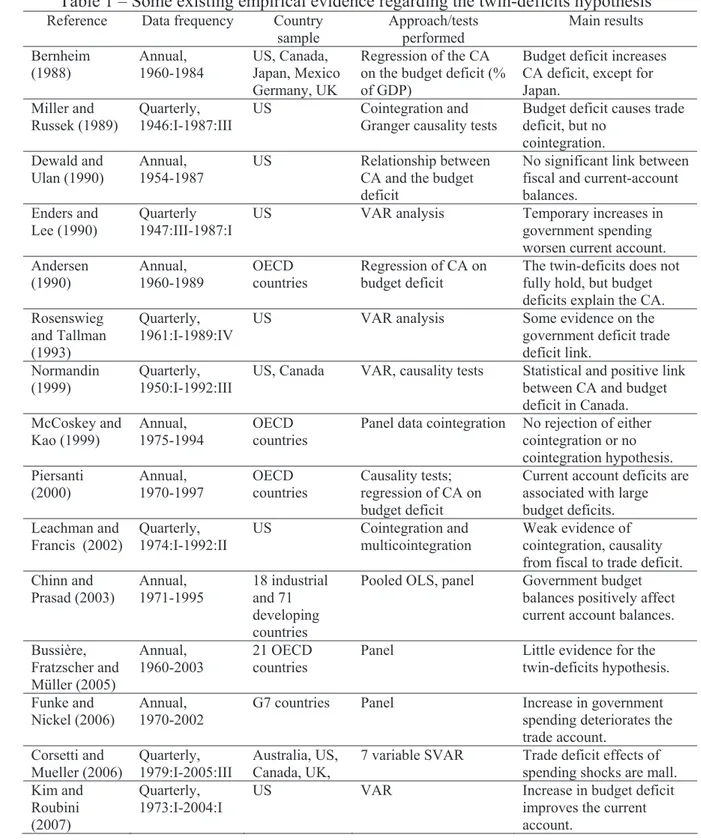
As already mentioned, empirical analysis does not necessarily provide a positive correlation between the budget balance and the current account balance. Indeed, the existing evidence is rather dissimilar, notably regarding single equation analysis, in the sense that budget balance deteriorations may hardly impinge on the current account position. Overall there is some mixed evidence in favour of a twin-deficits relationship (see Table 1 for a non-exhaustive overview), but this is neither robust nor stable over

6_{With perfect capital mobility, fiscal policy cannot restore the internal balance (Mundell, 1963).} 7

Since the effect on the balance of payments of exchange rate developments depends on more complicated mechanisms, see Obstfeld and Rogoff (1995), an empirical assessment is necessary.

8

Feldstein (1992) emphasises this point.

(15)

time, which may imply that fiscal tightening may not diminish the current account deficit.

Table 1 – Some existing empirical evidence regarding the twin-deficits hypothesis

Reference Data frequency Country sample Approach/tests performed Main results Bernheim (1988) Annual, 1960-1984 US, Canada, Japan, Mexico Germany, UK

Regression of the CA on the budget deficit (% of GDP)

Budget deficit increases CA deficit, except for Japan.

Miller and Russek (1989)

Quarterly, 1946:I-1987:III

US Cointegration and

Granger causality tests

Budget deficit causes trade deficit, but no

cointegration. Dewald and

Ulan (1990)

Annual, 1954-1987

US Relationship between

CA and the budget deficit

No significant link between fiscal and current-account balances.

Enders and Lee (1990)

Quarterly 1947:III-1987:I

US VAR analysis Temporary increases in government spending worsen current account. Andersen (1990) Annual, 1960-1989 OECD countries

Regression of CA on budget deficit

The twin-deficits does not fully hold, but budget deficits explain the CA. Rosenswieg

and Tallman (1993)

Quarterly, 1961:I-1989:IV

US VAR analysis Some evidence on the government deficit trade deficit link.

Normandin (1999)

Quarterly, 1950:I-1992:III

US, Canada VAR, causality tests Statistical and positive link between CA and budget deficit in Canada. McCoskey and Kao (1999) Annual, 1975-1994 OECD countries

Panel data cointegration No rejection of either cointegration or no cointegration hypothesis. Piersanti (2000) Annual, 1970-1997 OECD countries Causality tests; regression of CA on budget deficit

Current account deficits are associated with large budget deficits. Leachman and

Francis (2002)

Quarterly, 1974:I-1992:II

US Cointegration and

multicointegration

Weak evidence of cointegration, causality from fiscal to trade deficit. Chinn and Prasad (2003) Annual, 1971-1995 18 industrial and 71 developing countries

Pooled OLS, panel Government budget balances positively affect current account balances.

Bussière, Fratzscher and Müller (2005) Annual, 1960-2003 21 OECD countries

Panel Little evidence for the twin-deficits hypothesis.

Funke and Nickel (2006)

Annual, 1970-2002

G7 countries Panel Increase in government spending deteriorates the trade account. Corsetti and Mueller (2006) Quarterly, 1979:I-2005:III Australia, US, Canada, UK,

7 variable SVAR Trade deficit effects of spending shocks are mall. Kim and

Roubini (2007)

Quarterly, 1973:I-2004:I

US VAR Increase in budget deficit

(16)

3. Empirical analysis

Following some of the empirical strategy existing in the literature, one may recall expression (4) as depicting the basis of the twin-deficits idea. Therefore, assessing such hypothesis would involve testing the cointegration regression between the current account balance and the budget balance10, in a panel framework, as follows,

it i i it it

CA D E BUD u (6)

where the index i

i 1,...,N

denotes the country, the index t

t 1,...,T

indicates the period. Under such a framework, we can test for the existence of a long-term relationship, implying a positive effect of the budget balance to the current account balance. The possibility of effects from the current account balance to the budget balance (i.e. current account deteriorations lead to higher budget deficits via lower growth) could of course also be assessed, but we are at this stage more interested in the former relationship.

Moreover, a more encompassing specification that takes the effect of the real effective exchange rate (REX) on the current account balance into account can also be assessed:

it i i it i it it

CA D E BUD G REX u . (7) As already mentioned and according to the literature, the real effective exchange

rate can either have a positive or a negative effect on the current account, but its presence in a cointegration relationship such as in (7) cannot be discarded with certainty. Of course, additional factors can also be relevant for the developments of the current account balances. For instance, countries with a higher percentage share of older-age people in the population may have lower savings and higher consumption

10

(17)

spending, which could translate into a larger current account deficit, while the exchange rate regime will also play a role. However, we are essentially interested in focussing on the long-term relationship between the budgetary and current balances.

3.1. Data

All data for current account balances, general government budget balances and real effective exchange rates are taken from the European Commission AMECO (Annual Macro-Economic Data) database, from the IMF and from the OECD databases.11 We consider five different country panels: EU15, EU25, Cgroup21, Cgroup26, and Cgroup36. The data cover the periods from 1970 to 2007 respectively for the EU15 countries; from 1996 to 2007 for the EU25 countries (i.e. EU27 without Cyprus and Romania, due to short time span availability); from 1970 to 2007 for the Cgroup21 (i.e. EU15 and Australia, Canada, Iceland, Japan, Norway, USA); from 1987 to 2007 for Cgroup26 (i.e. EU15 and Australia, Canada, Iceland, Japan, Korea, Mexico, New-Zealand, Norway, Switzerland, Turkey, USA), and from 1996 to 2007 for Cgroup36 (i.e. EU25 and Australia, Canada, Iceland, Japan, Korea, Mexico, New-Zealand, Norway, Switzerland, Turkey, USA).12 These time spans are used both for the panel unit root tests and for the panel cointegration analysis. On the other hand, and as explained in sub-section 3.4, the unbalanced panels within the period 1970-2007 are used for the SUR analysis.

11

The AMECO codes are the following ones: .1.0.319.0.ublge, Net lending (+) or net borrowing (-): general government, % of GDP at market prices - excessive deficit procedure). .1.0.310.0.UBCA, Balance on current transactions with the rest of the world (National accounts), % of gross domestic product at market prices.

12_{Note that regarding the selection of the country groups, we use all OECD countries, just the EU15}

(18)

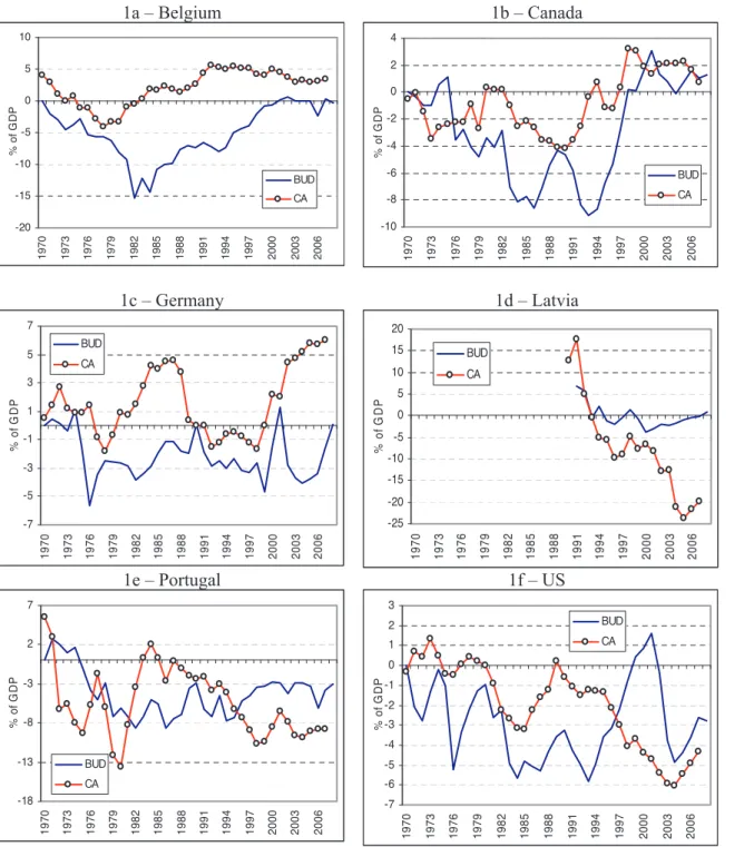
In Figure 1 we show a visual illustration of the budgetary and external balances for some of the countries included in our sample (a set of summary statistics is reported in Appendix B).

Figure 1 – Budgetary and external balances (% of GDP)

1a – Belgium 1b – Canada

-20 -15 -10 -5 0 5 10 19 70 19 73 19 76 19 79 19 82 19 85 19 88 19 91 19 94 19 97 20 00 20 03 20 06 % o f G D P BUD CA -10 -8 -6 -4 -2 0 2 4

1970 1973 1976 1979 1982 1985 1988 1991 1994 1997 2000 2003 2006

% o f G D P BUD CA

1c – Germany 1d – Latvia

-7 -5 -3 -1 1 3 5 7

1970 1973 1976 1979 1982 1985 1988 1991 1994 1997 2000 2003 2006

% o f G D P BUD CA -25 -20 -15 -10 -5 0 5 10 15 20

1970 1973 1976 1979 1982 1985 1988 1991 1994 1997 2000 2003 2006

% o

f GD

P

BUD

CA

1e – Portugal 1f – US

-18 -13 -8 -3 2 7 197 0 197 3 197 6 197 9 198 2 198 5 198 8 199 1 199 4 199 7 200 0 200 3 200 6 % o f G D P BUD CA -7 -6 -5 -4 -3 -2 -1 0 1 2 3

1970 1973 1976 1979 1982 1985 1988 1991 1994 1997 2000 2003 2006

% o f G D P BUD CA

(19)

3.2. 2nd generation panel unit root analysis

The literature on panel unit root and panel cointegration testing has been increasing considerably in the past years and now distinguishes between the first generation tests (see Maddala, and Wu, 1999; Levin, Lin and Chu, 2002; Im, Pesaran and Shin, 2003) developed on the assumption of the cross-sectional independence among panel units (except for common time effects), the second generation tests (e.g. Bai and Ng, 2004; Smith et al., 2004; Moon and Perron, 2004; Choi, 2006; Pesaran, 2007) allowing for a variety of dependence across the different units, and also panel data unit root tests that enable to accommodate structural breaks (e.g. Im and Lee, 2001). In addition, in recent years it has become more widely recognized that the advantages of panel data methods within the macro-panel setting include the use of data for which the spans of individualtime series data are insufficient for the study of many hypotheses of interest.

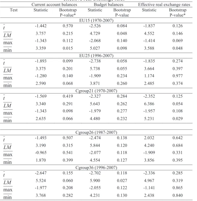
To determine the degree of integration of our series of interest (current account balances, budget balances and real effective exchange rates) in our five panel sets, we employ the bootstrap tests of Smith et al. (2004), which use a sieve sampling scheme to account for both the time series and cross-sectional dependencies of the data.13 The tests that we consider are denoted t, LM , max, and min . All four tests are constructed with a unit root under the null hypothesis and heterogeneous autoregressive roots under the alternative, which indicates that a rejection should be taken as evidence in favour of stationarity for at least one country.14 The results, reported in Table 1, suggest that for the series of the current account balances, budget balances and effective real exchange rates the unit root null cannot be rejected at any conventional significance level for most

13

We are grateful to Vanessa Smith for making available the Gauss codes of this test, which we adapted here for our purpose.

14

(20)

of the four tests.15 We therefore conclude that the variables are nonstationary in our country panels.

Table 1 – Panel unit root test for current account balances, budget balances and effective real exchange rates #

Current account balances Budget balances Effective real exchange rates Test Statistic Bootstrap

P-value*

Statistic Bootstrap P-value

Statistic Bootstrap P-value* EU15 (1970-2007)

t -1.442 0.570 -2.526 0.084 -1.837 0.126

LM 3.757 0.215 4.729 0.048 4.552 0.146

max -1.343 0.112 -2.068 0.140 -1.414 0.069

min 3.359 0.015 5.027 0.098 3.588 0.048

EU25 (1996-2007)

t -1.893 0.099 -2.738 0.058 -1.835 0.274

LM 3.375 0.201 5.738 0.055 3.664 0.397

max -1.280 0.140 -1.909 0.234 1.174 0.977

min 2.590 0.068 3.871 0.260 2.485 0.374

Cgroup21 (1970-2007)

t -1.569 0.419 -2.327 0.284 -2.352 0.125

LM 3.340 0.291 5.643 0.262 6.386 0.054

max -1.343 0.098 -1.979 0.277 -1.957 0.108

min 2.635 0.066 4.480 0.232 5.231 0.029

Cgroup26 (1987-2007)

t -1.493 0.507 -2.474 0.138 2.032 0.642

LM 3.190 0.315 5.844 0.120 4.240 0.684

max -0.965 0.541 -2.077 0.118 -1.909 0.331

min 1.870 0.399 4.554 0.127 3.856 0.395

Cgroup36 (1996-2007)

t -2.647 0.155 -2.702 0.118 -2.336 0.285

LM 5.524 0.060 5.900 0.027 4.967 0.319

max -1.977 0.208 -2.055 0.122 -1.141 0.865

min 3.768 0.282 4.231 0.130 2.438 0.840

Notes:

a) Rejection of the null hypothesis indicates stationarity at least in one country. All tests are based on an intercept and 5000 bootstrap replications to compute the p-values.

b) EU25 countries includes EU27 without Cyprus and Romania; group21 includes EU15 and Australia, Canada, Iceland, Japan, Norway, USA; Cgroup26 includes EU15 and Australia, Canada, Iceland, Japan, Korea, Mexico, New-Zealand, Norway, Switzerland, Turkey, USA; and Cgroup36 includes EU25 and Australia, Canada, Iceland, Japan, Korea, Mexico, New-Zealand, Norway, Switzerland, Turkey, USA. # Results based on the test of Smith et al. (2004).

15

(21)

3.3. Panel cointegration

We now proceed by testing for the existence of cointegration between current account balances and budget balances and also between current account balances, budget balances and effective real exchange rates (in conjecture with equations 6 and 7), using the bootstrap panel cointegration test proposed by Westerlund and Edgerton (2007). Unlike the panel data cointegration tests of Pedroni (1999, 2004), generalized by Banerjee and Carrion-i-Silvestre (2006), this test has the appealing advantage that the joint null hypothesis is cointegration for all countries in the panel. Therefore, in case of non rejection of the null, we can assume that a cointegration relationship for the whole set of countries of the panel exists, which is crucial to assess the twin-deficits hypothesis. On the contrary, performing the Banerjee and Carrion-i-Silvestre (2006) methodology raises the problem that a single series from the panel might be responsible for rejecting the joint null of non-stationary or non-cointegration, hence not necessarily implying that a cointegration relationship holds for the whole set of countries. This could be less helpful to investigate the two imbalances relationship since no information is provided on which panel members are responsible for this rejection, that is, for which country the cointegration relationship does not hold.

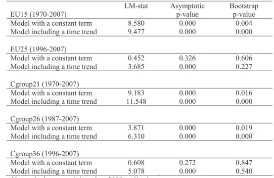
The test developed by Westerlund and Edgerton (2007) relies on the popular Lagrange multiplier test of McCoskey and Kao (1998), and permits correlation to be accommodated both within and between the individual cross-sectional units. In addition, this bootstrap test is based on the sieve-sampling scheme, and has the advantage of significantly reducing the distortions of the asymptotic test.16 The panel cointegration results reported in Table 2 for a model including either a constant term or a linear trend, clearly indicate the absence of a cointegrating relationship between

16

(22)

current account balances and budget balances for three panels sets out of five (EU15, Cgroup21, Cgroup26). This result is valid for any specification of the deterministic component considered, and is robust to the critical value used (asymptotic or bootstrap) for the conventional levels of significance. On the contrary, for the EU25 and Cgroup36 panel sets cointegration is detected for a model including a constant term in the EU25 panel set and for a model including either a constant term or a linear trend in the Cgroup36 panel set using bootstrap critical values.

Table 2 – Panel cointegration test results between current account balances and budget balances#

EU15 (1970-2007)

LM-stat Asymptotic p-value

Bootstrap p-value Model with a constant term 8.580 0.000 0.004 Model including a time trend 9.477 0.000 0.000

EU25 (1996-2007)

Model with a constant term 0.452 0.326 0.606 Model including a time trend 3.685 0.000 0.227

Cgroup21 (1970-2007)

Cgroup26 (1987-2007)

Cgroup36 (1996-2007)

Notes: the bootstrap is based on 2000 replications.

a - The null hypothesis of the tests is cointegration between current account balances and budget balances.

b) EU25 countries includes EU27 without Cyprus and Romania; Cgroup21includes EU15 and Australia, Canada, Iceland, Japan, Norway, USA; Cgroup26 includes EU15 and Australia, Canada, Iceland, Japan, Korea, Mexico, New-Zealand, Norway, Switzerland, Turkey, USA; and Cgroup36 includes EU25 and Australia, Canada, Iceland, Japan, Korea, Mexico, New-Zealand, Norway, Switzerland, Turkey, USA.

# Test based on Westerlund and Edgerton (2007).

(23)

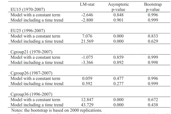
produces significant evidence in favour of the existence of a cointegration relationship for three panels sets out of five (EU15, Cgroup21, Cgroup26) for any specification of the deterministic component considered if one relies on asymptotic p-values. Results are even stronger when using bootstrap p-values since the null hypothesis of cointegration cannot be rejected for the five panel sets for any specification of the deterministic component considered. These results underline the crucial importance of considering the effect of the effective real exchange rate in assessing the twin cointegration between budgetary and current account balances.

Table 3 – Panel cointegration test results between current account balances, budget balances and effective real exchange rates #

EU15 (1970-2007)

LM-stat Asymptotic p-value

Bootstrap p-value Model with a constant term -2.646 0.848 0.996 Model including a time trend -2.800 0.901 0.999

EU25 (1996-2007)

Cgroup21 (1970-2007)

Model with a constant term -1.075 0.859 0.999 Model including a time trend -3.366 0.892 0.998

Cgroup26 (1987-2007)

Cgroup36 (1996-2007)

Notes: the bootstrap is based on 2000 replications.

a - The null hypothesis of the tests is cointegration between current account balances, budget balances and effective real exchange rates.

b) EU25 countries includes EU27 without Cyprus and Romania; Cgroup21includes EU15 and Australia, Canada, Iceland, Japan, Norway, USA; Cgroup26 includes EU15 and Australia, Canada, Iceland, Japan, Korea, Mexico, New-Zealand, Norway, Switzerland, Turkey, USA; and Cgroup36 includes EU25 and Australia, Canada, Iceland, Japan, Korea, Mexico, New-Zealand, Norway, Switzerland, Turkey, USA.

(24)

3.4. SUR cointegration relationships

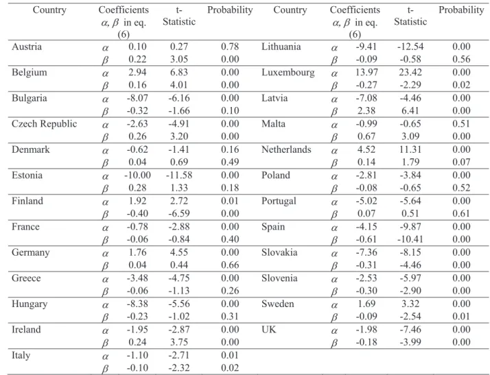
If a cointegrating relationship exists for all countries of a given panel set, we estimate the systems (6) and (7) by the Zellner (1962) approach to handle cross-sectional dependence among countries using the SUR estimator. It is now well known that the presence of cross-section dependence renders the ordinary least squares estimator inefficient and biased, which makes it a poor candidate for inference. A common approach to alleviate this problem is to use Seemingly Unrelated Regressions techniques. However, as noted by Westerlund (2007), this approach is not feasible when the cross-sectional dimension N is of the same order of magnitude as the time series dimension, since the covariance matrix of the regression errors then becomes rank deficient. In fact, for the SUR approach to work properly, one usually requires the time series dimension being substantially larger than N, a condition that is only fulfilled for the EU15 and Cgroup21 panels over the 1970-2007 period, but not for the EU25, Cgroup26, and Cgroup36 panels over the 1996-2007, 1987-2007 and 1996-2007 periods. As a consequence, for the last three panels the SUR estimation technique is actually performed on the (unbalanced) 1970-2007 period, according to data availability. This way of proceeding enables us to estimate the individual coefficients ȕi

(25)

Table 4a – SUR estimation for the EU25 panel (1970-2007)

Country Coefficients

DE in eq. (6)

t-Statistic

Probability Country Coefficients

DE in eq. (6)

t-Statistic

Probability

Austria D 0.10 0.27 0.78 Lithuania D -9.41 -12.54 0.00

E 0.22 3.05 0.00 E -0.09 -0.58 0.56

Belgium D 2.94 6.83 0.00 Luxembourg D 13.97 23.42 0.00

E 0.16 4.01 0.00 E -0.27 -2.29 0.02

Bulgaria D -8.07 -6.16 0.00 Latvia D -7.08 -4.46 0.00

E -0.32 -1.66 0.10 E 2.38 6.41 0.00

Czech Republic D -2.63 -4.91 0.00 Malta D -0.99 -0.65 0.51

E 0.26 3.20 0.00 E 0.67 3.09 0.00

Denmark D -0.62 -1.41 0.16 Netherlands D 4.52 11.31 0.00

E 0.04 0.69 0.49 E 0.14 1.79 0.07

Estonia D -10.00 -11.58 0.00 Poland D -2.81 -3.84 0.00

E 0.28 1.33 0.18 E -0.08 -0.65 0.52

Finland D 1.92 2.72 0.01 Portugal D -5.02 -5.64 0.00

E -0.40 -6.59 0.00 E 0.07 0.51 0.61

France D -0.78 -2.88 0.00 Spain D -4.15 -9.87 0.00

E -0.06 -0.84 0.40 E -0.61 -10.41 0.00

Germany D 1.76 4.55 0.00 Slovakia D -7.36 -8.15 0.00

E 0.04 0.44 0.66 E -0.31 -4.46 0.00

Greece D -3.48 -4.75 0.00 Slovenia D -2.53 -5.97 0.00

E -0.06 -1.13 0.26 E -0.30 -2.90 0.00

Hungary D -8.38 -5.56 0.00 Sweden D 1.69 3.32 0.00

E -0.23 -1.02 0.31 E -0.09 -2.54 0.01

Ireland D -1.95 -2.87 0.00 UK D -1.98 -7.46 0.00

E 0.24 3.75 0.00 E -0.18 -3.99 0.00

Italy D -1.10 -2.71 0.01

E -0.10 -2.32 0.02

Note: Seemingly Unrelated Regression, linear estimation after one-step weighting matrix. Unbalanced system, total observations: 718.

(26)

feature, both regarding the sign of the estimated effect of budget balances on current account balances and regarding its absolute magnitude, but there is no evidence pointing to a close relationship. We also assessed the homogeneity of ȕi across country using a

Wald test, but such null hypothesis was rejected.

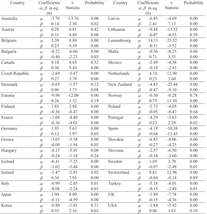
Table 4b – SUR estimation for the Cgroup36 panel (1970-2007)

DE in eq. (6)

t-Statistic

Probability Country Coefficients

DE in eq. (6)

t-Statistic

Probability

Australia D -3.70 -13.76 0.00 Latvia D -6.85 -4.69 0.00

E 0.14 2.30 0.02 E 2.41 7.13 0.00

Austria D 0.28 0.81 0.42 Lithuania D -9.44 -13.52 0.00

E 0.31 4.80 0.00 E -0.07 -0.55 0.59

E 0.25 9.39 0.00 E -0.31 -3.52 0.00

Bulgaria D -8.22 -6.66 0.00 Malta D -0.36 -0.25 0.80

E -0.40 -2.23 0.03 E 0.71 3.55 0.00

Canada D 0.18 0.65 0.52 Mexico D -2.49 -4.38 0.00

E 0.30 9.43 0.00 E -0.19 -2.93 0.00

Czech Republic D -2.69 -5.47 0.00 Netherlands D 4.74 12.90 0.00

E 0.27 3.78 0.00 E 0.23 3.60 0.00

Denmark D -0.65 -1.57 0.12 New Zealand D -4.83 -23.44 0.00

E 0.06 1.73 0.08 E -0.47 -9.10 0.00

Estonia D -9.98 -12.08 0.00 Norway D -0.30 -0.28 0.78

E 0.26 1.32 0.19 E 0.75 11.10 0.00

Finland D 1.83 2.88 0.00 Poland D -2.73 -4.05 0.00

E -0.36 -8.47 0.00 E -0.05 -0.47 0.64

France D -1.04 -4.40 0.00 Portugal D -4.29 -5.63 0.00

E -0.16 -4.02 0.00 E 0.23 2.29 0.02

Germany D 1.93 5.63 0.00 Spain D -4.19 -10.38 0.00

E 0.12 1.97 0.05 E -0.64 -13.43 0.00

Greece D -3.65 -5.38 0.00 Slovakia D -6.83 -8.06 0.00

E -0.09 -1.94 0.05 E -0.27 -4.25 0.00

Hungary D -8.17 -5.91 0.00 Slovenia D -2.57 -6.50 0.00

E -0.24 -1.18 0.24 E -0.34 -3.60 0.00

Iceland D -6.41 -7.25 0.00 Sweden D 1.69 3.70 0.00

E -1.02 -5.44 0.00 E -0.07 -2.49 0.01

Ireland D -1.47 -2.41 0.02 Switzerland D 8.61 12.96 0.00

E 0.34 7.93 0.00 E -0.04 -0.14 0.89

Italy D -0.99 -2.65 0.01 Turkey D -5.18 -8.01 0.00

E -0.08 -2.24 0.03 E -0.15 -2.49 0.01

Japan D 1.90 8.09 0.00 UK D -1.89 -7.78 0.00

E -0.11 -4.59 0.00 E -0.15 -4.36 0.00

Korea D -0.80 -1.01 0.31 USA D -1.84 -5.92 0.00

E 0.55 2.16 0.03 E 0.06 1.63 0.10

(27)

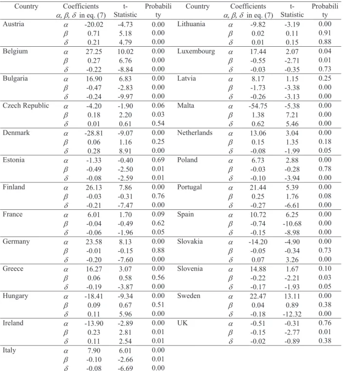
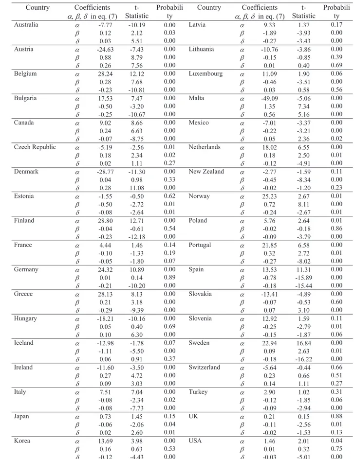
For the case of the relationship between budgetary and current account balances, and the effective real exchange rate the results are reported in Tables 4c, 4d and 4e, respectively for country groups EU15, EU25, and Cgroup36.17

Table 4c – SUR estimation for the EU15 panel (1970-2007)

DEG in eq. (7) t-Statistic

Probabili ty

Austria D -19.76 -4.47 0.00 Italy D 7.84 5.76 0.00

E 0.68 4.74 0.00 E -0.10 -2.58 0.01

G 0.21 4.52 0.00 G -0.08 -6.41 0.00

E 0.27 6.31 0.00 E -0.53 -2.54 0.01

G -0.22 -8.25 0.00 G -0.03 -0.33 0.74

E 0.07 1.18 0.24 E 0.13 1.18 0.24

G 0.28 8.40 0.00 G -0.08 -1.98 0.05

Finland D 25.48 7.50 0.00 Portugal D 20.95 5.10 0.00

E -0.04 -0.36 0.72 E 0.23 1.56 0.12

G -0.21 -7.09 0.00 G -0.27 -6.32 0.00

France D 6.25 1.68 0.09 Spain D 10.48 5.91 0.00

E -0.03 -0.32 0.75 E -0.73 -10.23 0.00

G -0.06 -1.91 0.06 G -0.14 -8.52 0.00

Germany D 23.06 7.47 0.00 Sweden D 22.60 13.00 0.00

E -0.04 -0.43 0.67 E 0.05 0.94 0.35

G -0.20 -6.99 0.00 G -0.18 -12.23 0.00

Greece D 13.83 2.46 0.01 UK D -0.32 -0.18 0.86

E 0.03 0.28 0.78 E -0.14 -2.44 0.01

G -0.16 -3.21 0.00 G -0.02 -0.93 0.35

Ireland D -13.21 -2.70 0.01

E 0.22 2.69 0.01

G 0.10 2.35 0.02

Note: Seemingly Unrelated Regression, linear estimation after one-step weighting matrix. Balanced system, total observations: 570.

According to the SUR results there is a statistically significant effect of the real effective exchange rate on the current account balance for the majority of the countries. Some exceptions occur for the cases of Luxembourg and the UK in the EU15 panel, for the Czech Republic, Lithuania, Luxembourg and the UK in the EU25 panel, and for The Czech Republic, Iceland, Lithuania, Luxembourg, New Zealand, Switzerland and the UK in the Cgroup36 panel.

17

(28)

Table 4d – SUR estimation for the EU25 panel (1970-2007)

Probabili ty

Austria D -20.02 -4.73 0.00 Lithuania D -9.82 -3.19 0.00

E 0.71 5.18 0.00 E 0.02 0.11 0.91

G 0.21 4.79 0.00 G 0.01 0.15 0.88

E 0.27 6.76 0.00 E -0.55 -2.71 0.01

G -0.22 -8.84 0.00 G -0.03 -0.35 0.73

Bulgaria D 16.90 6.83 0.00 Latvia D 8.17 1.15 0.25

E -0.47 -2.83 0.00 E -1.73 -3.38 0.00

G -0.24 -9.97 0.00 G -0.26 -3.13 0.00

Czech Republic D -4.20 -1.90 0.06 Malta D -54.75 -5.38 0.00

E 0.18 2.20 0.03 E 1.38 7.21 0.00

G 0.01 0.61 0.54 G 0.62 5.46 0.00

E 0.06 1.16 0.25 E 0.15 1.35 0.18

G 0.28 8.91 0.00 G -0.08 -1.99 0.05

Estonia D -1.33 -0.40 0.69 Poland D 6.73 2.88 0.00

E -0.49 -2.50 0.01 E -0.03 -0.28 0.78

G -0.08 -2.59 0.01 G -0.10 -3.94 0.00

E -0.03 -0.31 0.76 E 0.25 1.76 0.08

G -0.21 -7.47 0.00 G -0.27 -6.61 0.00

France D 6.01 1.70 0.09 Spain D 10.72 6.25 0.00

E -0.04 -0.49 0.62 E -0.74 -10.68 0.00

G -0.06 -1.96 0.05 G -0.15 -8.98 0.00

Germany D 23.58 8.13 0.00 Slovakia D -14.20 -4.90 0.00

E -0.01 -0.15 0.88 E -0.05 -0.34 0.73

G -0.20 -7.60 0.00 G 0.07 3.26 0.00

Greece D 16.27 3.07 0.00 Slovenia D 14.88 1.67 0.10

E 0.06 0.58 0.56 E -0.22 -2.21 0.03

G -0.19 -3.87 0.00 G -0.17 -1.93 0.05

Hungary D -18.41 -9.34 0.00 Sweden D 22.47 13.11 0.00

E 0.09 0.67 0.51 E 0.04 0.89 0.38

G 0.11 5.96 0.00 G -0.18 -12.32 0.00

Ireland D -13.90 -2.89 0.00 UK D -0.51 -0.31 0.76

E 0.23 2.81 0.01 E -0.15 -2.77 0.01

G 0.11 2.54 0.01 G -0.02 -0.89 0.38

Italy D 7.90 6.01 0.00

E -0.10 -2.66 0.01

G -0.08 -6.69 0.00

(29)

Table 4e – SUR estimation for the Cgroup36 panel (1970-2007)

Probabili ty

Probabili ty Australia D -7.77 -10.19 0.00 Latvia D 9.33 1.37 0.17

E 0.12 2.12 0.03 E -1.89 -3.93 0.00

G 0.03 5.51 0.00 G -0.27 -3.43 0.00

Austria D -24.63 -7.43 0.00 Lithuania D -10.76 -3.86 0.00

E 0.88 8.79 0.00 E -0.15 -0.85 0.39

G 0.26 7.56 0.00 G 0.01 0.40 0.69

E 0.28 7.68 0.00 E -0.46 -3.51 0.00

G -0.23 -10.81 0.00 G 0.03 0.58 0.56 Bulgaria D 17.53 7.47 0.00 Malta D -49.09 -5.06 0.00

E -0.50 -3.20 0.00 E 1.35 7.34 0.00

G -0.25 -10.67 0.00 G 0.56 5.16 0.00 Canada D 9.02 8.66 0.00 Mexico D -7.01 -3.37 0.00

E 0.24 6.63 0.00 E -0.22 -3.21 0.00

G -0.07 -8.75 0.00 G 0.05 2.36 0.02

Czech Republic D -5.19 -2.56 0.01 Netherlands D 18.02 6.55 0.00

E 0.18 2.34 0.02 E 0.18 2.50 0.01

G 0.02 1.11 0.27 G -0.12 -4.91 0.00

E 0.04 0.98 0.33 E -0.45 -8.34 0.00

G 0.28 11.08 0.00 G -0.02 -1.20 0.23 Estonia D -1.55 -0.50 0.62 Norway D 25.23 2.67 0.01

E -0.50 -2.72 0.01 E 0.72 8.11 0.00

G -0.08 -2.64 0.01 G -0.24 -2.67 0.01 Finland D 28.80 12.71 0.00 Poland D 5.76 2.64 0.01

E -0.04 -0.61 0.54 E -0.02 -0.18 0.86

G -0.23 -12.18 0.00 G -0.09 -3.79 0.00 France D 4.44 1.46 0.14 Portugal D 21.85 6.58 0.00

E -0.10 -1.33 0.19 E 0.32 2.72 0.01

G -0.05 -1.80 0.07 G -0.27 -8.02 0.00 Germany D 24.32 10.89 0.00 Spain D 13.53 11.31 0.00

E 0.01 0.14 0.89 E -0.78 -15.89 0.00

G -0.21 -10.20 0.00 G -0.18 -15.44 0.00 Greece D 28.13 8.13 0.00 Slovakia D -13.41 -4.89 0.00

E 0.21 3.18 0.00 E -0.07 -0.53 0.60

G -0.29 -9.39 0.00 G 0.07 3.10 0.00

Hungary D -18.21 -10.16 0.00 Slovenia D 12.92 1.59 0.11

E 0.05 0.40 0.69 E -0.25 -2.79 0.01

G 0.10 6.30 0.00 G -0.15 -1.87 0.06

Iceland D -12.98 -1.78 0.07 Sweden D 22.94 16.84 0.00

E -1.11 -5.50 0.00 E 0.09 2.63 0.01

G 0.06 0.91 0.37 G -0.18 -16.22 0.00 Ireland D -11.60 -3.50 0.00 Switzerland D -5.64 -0.44 0.66

E 0.27 4.72 0.00 E 0.23 0.66 0.51

G 0.09 3.03 0.00 G 0.14 1.11 0.27

Italy D 7.51 7.04 0.00 Turkey D 2.90 1.02 0.31

E -0.08 -2.34 0.02 E -0.12 -1.85 0.06

G -0.08 -7.73 0.00 G -0.09 -2.94 0.00 Japan D 0.73 1.45 0.15 UK D 0.21 0.15 0.88

E -0.06 -2.06 0.04 E -0.11 -2.56 0.01

G 0.02 2.60 0.01 G -0.02 -1.53 0.13

Korea D 13.69 3.98 0.00 USA D 1.46 2.01 0.04

E 0.16 0.63 0.53 E 0.01 0.32 0.75

(30)

Table 5 summarises the SUR results regarding the sign of the E coefficient (the effect between budget balances and current account balances) for the EU15 and Cgroup36 panels, both for the specification without and with the effective real exchange rate. In addition, Figure 2 illustrates the statistically significant estimated E coefficients for each country, regarding the results for the Cgroup36 panel.

Table 5 – Sign of estimated E in (6), CA_it D E_i _iBUD_it u_it, and in (7),

it i i it i it it

CA D E BUD G REX u ,10% significance

Country panel

Regression Sign

ofE

Countries

+ AU, BE, CZ, IR, LV, MT

eq (6)

- FI, IT, LU, SP, SK, SL, SW, UK

+ AU, BE, IR

EU15

eq (7)

- IT, LU, SP, UK

+ AUS, AU, BE, CAN, CZ, DE, IR, KOR, LV, MT,

NL, NOR, PT eq (6)

- BG, FI, FR, GR, IT, IC, JP, LU, SP, SK, SL, SW, TR,

UK

+ AUS, AU, BE, CAN, CZ, GR, IR, MT, NL, NOR, PT,

SW Cgroup36

eq (7)

- BG, ET, IT, IC, JP, LV, LU, MEX, NZ, SP, SL, UK

Figure 2 – Estimated E coefficient in (7), statistically significant at 10%, Cgroup36 panel (1970-2007) -2.0 -1.5 -1.0 -0.5 0.0 0.5 1.0 1.5 La tv ia Ic e la n d S pai n B u lg a ria Es to n ia Lu x em b our g New Z e al an d S lov eni a M e xi co Tu rk e y

UK _Italy

(31)

To assess the relevance of possible different regimes notably in the run-up to the EMU we performed a similar analysis for the EU15 panel for two sub-periods, 1970-1989 and 1990-2007. The results, reported in Appendix D, show significant evidence in favour of the existence of a unit root in the current account balances, budget balances and effective real exchange rates series for the two sub-periods, which is in line with what we found for the full 1970-2007 period. Moreover, we are now able to find a significant cointegrating relationship between current account balances and budget balances for the sub-period 1990-2007, which was not the case for the full sample. It is also possible to confirm the relevant role of the effective real exchange rates in a long-run relationship between current account balances, budget balances and effective real exchange rates series for the two sub-periods.

Finally, the SUR estimations confirm the existence of different effects of budget balances and effective real exchange rates on the current account balances for the sub-periods 1970-1989 and 1990-2007. Interestingly, the results also show that the estimated relationship between budget balances and current account balances, which was positive in the first sub-period, became negative in the second sub-period for Belgium, France, Greece, and Portugal.18 To our mind, this may reveals different economic phases, before and after 1990. For instance, one observed a decline in private-sector saving rates in several OECD countries in the late 1990s, while fiscal consolidation efforts also occurred during that period in several EU countries.19

4. Conclusion

In this paper we assessed the existence of a cointegration relationship between current account and budget balances, and between current account, budget balances and

18

Kim and Roubini (2007) also find some evidence of such so-called twin-divergence.

19

(32)

effective real exchange rates, using recent bootstrap panel cointegration techniques and the Seemingly Unrelated Regression methods, which, to the best of our knowledge, was not employed before in this context. For the period from 1970 to 2007, and for different EU and OECD country groupings, we also investigate the magnitude of these relationships for each country. The results of the panel unit root tests that we performed suggest that for the series of the current account balances, budget balances and effective real exchange rates, the unit root null cannot be rejected at the usual significance levels for most of the tests.

On the basis of the stationarity results, we tested for the existence of cointegration between current account balances and budget balances and also between current account balances, budget balances and effective real exchange rates using the bootstrap panel cointegration test proposed by Westerlund and Edgerton (2007). For the EU25 and Cgroup36 panel sets cointegration is detected between budgetary and current account balances for a model including a constant term in the EU25 panel set, and for a model including either a constant term or a linear trend in the Cgroup36 panel, set using bootstrap critical values.

(33)

exchange rate in assessing the cointegration hypothesis between budgetary and current account balances.

The SUR analysis shows a statistically significant (at the 5 per cent level) positive effect of budget balances on current account balances for several EU countries: Austria, Belgium, Czech Republic, Ireland, Latvia, and Malta. On the other hand, a statistically significant (at the 5 per cent level) negative effect of budget balances on current account balances can be found for Finland, Italy, Luxembourg, Spain, Slovakia, Slovenia, Sweden and the UK, although the magnitude of the estimated E coefficient varies considerably across countries.

The country specific findings for the EU25 panel are essentially confirmed for the broader Cgroup36 panel. In addition, the heterogeneity of the results is the main feature, both regarding the sign of the estimated effect of budget balances on current account balances and regarding its absolute magnitude, but there is no evidence pointing to a close relationship. Therefore, additional factors other than fiscal policy contributed to the development of the current account balances of the countries in our sample, for instance, liquidity constraints in the international capital market, and different monetary policy regimes (see, for instance, Gruber and Kamin, 2007).

(34)

References

Afonso, A. and Rault, C. (2007). “What do we really know about fiscal sustainability in the EU? A panel data diagnostic”, ECB Working Paper 820.

Andersen, P. (1990). “Developments in external and internal balances: a selective and eclectic view”, BIS Economic Papers, 29.

Bai, J., Ng, S. (2004), "A PANIC Attack on Unit Roots and Cointegration",

Econometrica, 72 (4), 127-1177.

Banerjee, A. and Carrion-i-Silvestre, J. (2006). “Cointegration in Panel Data with Breaks and Cross-section Dependence”, European Central Bank, Working Paper 591, February.

Barro, R. (1974). “Are Government Bonds Net Wealth?” Journal of Political Economy, 82 (6), 1095-117.

Bernanke, B. (2005). “The Global Saving Glut and the U.S. Current Account Deficit,” Speech at the Homer Jones Lecture, St. Louis, Missouri, April 12, 2005.

Bernheim, B. (1988). “Budget Deficits and the Balance of Trade”, Tax Policy and the Economy, 2.

Bussière, M., Fratzscher, M. and Müller, G. (2005). “Productivity Shocks, Budget Deficits and the Current Account”, ECB Working Paper 509.

Campbell, J. and Perron, P. (1991). ‘‘Pitfalls and Opportunities: What Macroeconomists should know about Unit Roots,’’ in Blanchard, O. and Fisher, S. (eds.), NBER Macroeconomics Annual. Cambridge, MA: MIT Press.

Cherneff, R. (1976). “Policy Conflict and Coordination under Fixed Exchanges: The Case of an Upward Sloping is Curve”, Journal of Finance, 31 (4), 1219-1224.

Chinn, D. and Prasad, E. (2003). “Medium-term determinants of current accounts in industrial and developing countries: an empirical exploration”, Journal of International Economics, 59 (1), 47-76.

Chinn, M. and Wei, S.-J. (2008). “A Faith-based Initiative: Do We Really Know that a Flexible Exchange Rate Regime Facilitates Current Account Adjustment”, mimeo. Choi, I. (2006). “Combination Unit Root Tests for Cross-sectionally Correlated Panels”,

(35)

Corsetti, G. and Müller, G. (2006). “Twin Deficits: Squaring Theory, Evidence and Common Sense”, Economic Policy, 21 (48), 597-638.

De Serres, A. and Pelgrin, F. (2003). “The Decline in Private Saving Rates in the 1990s in OECD Countries: How Much Can Be Explained by Non-wealth Determinants?”

OECD Economics Studies No. 36, 2003/1.

Dewald, W. and Ulan, M. (1990). “The Twin Deficit-Illusion”, Cato Journal, 9 (3), 689-707.

Dornbusch, R. (1976). “Expectations and Exchange Rate Dynamics”, Journal of Political Economy, 84 (6), 1161-1176.

Enders, W. and Lee, B.-S. (1990). “Current Account and Budget Deficits: Twins or Distant Cousins?” Review of Economics and Statistics, 72 (3), 373-381.

Feldstein, M. and Horioka, C. (1980). “Domestic saving and International Capital Flows",Economic Journal, 90 (358), 314-329.

Feldstein, M. (1992). “The budget and trade deficits aren’t really twins”, NBER WP N. 3966.

Fleming, J. (1962). “Domestic Financial Policies under Fixed and Floating Exchange Rates,” IMF Staff Papers, 9, 369-379.

Frankel, J. (2006). “Twin Deficits and Twin Decades,” in Kopcke, R; Tootell, G. and Triest, R. (eds.), The Macroeconomics of Fiscal Policy, MIT Press: Cambridge MA. Funke, K. and Nickel, C. (2006). “Does fiscal policy matter for the trade account? A

panel cointegration study”, ECB Working Paper 620.

Gruber, J. and Kamin, S. (2007). “Explaining the global pattern of current account imbalances”, Journal of International Money and Finance, 26 (4), 500-522.

IMF (2007). “Review of Exchange Arrangements, Restrictions, and Controls”, November 27, IMF, Monetary and Capital Markets Department.

Im, K. and Lee, J. (2001). “Panel LM Unit Root Test with Level Shifts”, Discussion paper, Department of Economics, University of Central Florida.

Im, K., Pesaran, M. and Shin, Y. (2003). “Testing for Unit Roots in Heterogeneous Panels”,Journal of Econometrics, 115 (1), 53-74.

Kim, S. and Roubini, N. (2007). “Twin Deficits or Twin Divergence? Fiscal Policy, Current Account, and Real Exchange Rate in the U.S.”, forthcoming, Journal of International Economics.

(36)

Levin, A., Lin, C.-F. and Chu, C.-S. (2002). “Unit Root Tests in Panel Data: Asymptotic and Finite Sample Properties”, Journal of Econometrics, 108 (1), 1-24. Maddala, G. and Wu, S. (1999). “A Comparative Study of Unit Root Tests and a New

Simple Test”, Oxford Bulletin of Economics and Statistics, 61 (1), 631-652.

Mankiw, N. (2006). “Reflections on the trade deficit and fiscal policy”, Journal of Policy Modeling, 28, 679–682.

McCoskey, S. and Kao, C. (1998). “A Residual-Based Test of the Null of Cointegration in Panel Data”, Econometric Reviews, 17 (1), 57-84.

McCoskey, S. and Kao, C. (1999). “Comparing panel data cointegration tests with an application to the ‘twin deficits’ problem”, mimeo.

Miller, S. and Russek, F. (1989). “Are the Twin Deficits Really Related?”

Contemporary Economic Policy, 7 ( 4), 91-115.

Moon, H. and Perron, B. (2004). “Testing for a Unit Root in Panels with Dynamic Factors”,Journal of Econometrics, 122 (1), 8-126.

Mundell, R. (1963). “Capital Mobility and Stabilization Policy under Fixed and Flexible Exchange Rates,” Canadian Journal of Economics and Political Science, 29, 475-85.

Normandin, M. (1999). “Budget Deficit Persistence and the Twin Deficits Hypothesis”,

Journal of International Economics, 49 (1), 171-194.

Obstfeld, M. and Rogoff, K. (1995). “The Intertemporal Approach to the Current Account,” in Grossman, G. and Rogoff, K. (eds.) Handbook of International Economics. North-Holland.

Pedroni, P. (1999). “Critical Values for Cointegrating Tests in Heterogeneous Panels with Multiple Regressors”, Oxford Bulletin of Economics and Statistics, 61 (1), 653-670.

Pedroni, P. (2004). “Panel Cointegration; Asymptotic and Finite Sample Properties of Pooled Time Series Tests with an Application to the Purchasing Power Parity Hypothesis”,Econometric Theory, 20 (3), 597-625.

Pesaran, M. (2007). “A Simple Panel Unit Root Test in the Presence of Cross Section Dependence”,Journal of Applied Econometrics, 22 (2), 265-312.

(37)

Ricardo, D. (1817). On the Principles of Political Economy and Taxation, in P. Sraffa (ed.),The works and correspondence of David Ricardo, Volume I, 1951, Cambridge University Press, Cambridge.

Rosenswieg, J. and Tallman, E. (1993). “Fiscal Policy and Trade Adjustment: Are the Deficits Really Twins?” Economic Inquiry, 31(4), 580-594.

Roubini, N. (1988). “Current Account and Budget Deficits in an Intertemporal Model of Consumption and Taxation Smoothing: A solution to the ’Feldstein-Horioka Puzzle’?” NBER Working Paper 2773.

Smith, V., Leybourne, S. and Kim, T.-H. (2004). ‘‘More Powerful Panel Unit Root Tests with an Application to the Mean Reversion in Real Exchange Rates.’’ Journal of Applied Econometrics, 19 (2), 147–170.

Westerlund, J. and Edgerton, D. (2007). “A Panel Bootstrap Cointegration Test”,

Economics Letters, 97 (3), 185-190, 2007.

Westerlund, J. (2007). “Estimating Cointegrated Panels with Common Factors and the Forward Rate Unbiasedness Hypothesis”. Journal of Financial Econometrics, 5 (3), 491-522.

(38)

Appendix A – Text-book imbalances relationship

Figure A1 provides a standard text-book illustration to the link between the

budget and the current account balances with flexible exchanges rates in the

Fleming-Mundell Keynesian setup. Starting from the initial position at point A in Figure A1.a, a

fiscal expansion that increases the budget deficit shifts IS0 to the right to IS1 in B. At

point B, with a higher domestic interest rate, there is an inflow of capital and a surplus

vis-à-vis the exterior given that point B is above the BP curve. This will lead to an

appreciation of the domestic currency, moving BP0 upwards to BP1, which deteriorates

the current account. In turn, the appreciation drives the IS1 curve downwards to IS2,

intersecting the LM and the BP curves at point C. Moreover, one may also point out that

the need for the government to finance the budget deficit by issuing additional

government debt, which may be bought by foreign investors, will also increase interest

income outflows and contribute to deteriorate the external balance.

Figure A1– Fiscal policy and external position under flexible exchange rates

(39)

(40)

Appendix B – Summary statistics

Table B1 – Summary statistics (1970-2007)

Current account balance (% of GDP)

AUS AUT BEL BGR CAN CHE CZE DEU DNK ESP EST FIN Mean -3.9 -0.4 2.1 -7.1 -0.8 6.8 -3.5 1.7 -0.6 -2.7 -8.9 1.0 Max 1.4 5.3 5.6 3.5 3.3 17.5 1.7 6.0 3.6 1.5 1.2 10.0 Min -6.2 -5.2 -4.0 -18.1 -4.2 0.1 -6.7 -1.8 -5.5 -9.8 -15.7 -7.5 Std. Dev. 1.6 2.4 2.7 6.5 2.2 4.7 2.4 2.4 2.8 3.1 4.3 4.8

Observ. 38 38 38 19 38 38 18 38 38 38 17 38

FRA GBR GRC HUN IRL ISL ITA JPN KOR LTU LUX LVA Mean -0.6 -1.5 -3.2 -6.7 -2.9 -6.0 -0.4 2.2 -0.4 -9.0 13.4 -7.0 Max 2.5 1.9 3.1 -2.7 3.7 1.9 3.1 4.8 12.2 -3.1 25.1 17.8 Min -4.0 -5.1 -11.1 -9.6 -14.6 -26.7 -4.3 -1.1 -10.6 -14.6 7.8 -23.8 Std. Dev. 1.6 1.6 4.4 2.0 4.6 7.6 1.7 1.6 4.6 3.5 3.5 11.0

Observ. 38 38 38 17 38 38 38 38 38 16 38 19

MEX MLT NLD NOR NZL POL PRT SVK SVN SWE TUR USA Mean -2.4 -5.7 4.2 3.9 -5.1 -2.6 -5.3 -4.4 0.1 1.7 -4.2 -2.0 Max 5.3 2.5 8.6 17.4 1.9 2.3 5.5 5.3 8.5 7.3 1.5 1.3 Min -6.9 -12.5 -0.9 -12.3 -13.3 -6.2 -13.5 -9.4 -3.5 -2.6 -20.0 -6.1 Std. Dev. 3.0 3.9 2.3 8.0 2.7 2.4 4.4 4.1 3.3 3.3 4.5 2.1

Observ. 38 15 38 38 38 19 38 17 20 38 38 38

Budget balance (% of GDP)

AUS AUT BEL BGR CAN CHE CZE DEU DNK ESP EST FIN Mean -1.8 -2.1 -5.2 -1.3 -3.0 -0.8 -5.0 -2.2 0.1 -2.3 1.5 2.5 Max 2.3 1.9 0.6 5.3 3.0 2.2 -2.9 1.3 5.0 1.8 9.5 7.8 Min -5.4 -5.6 -15.3 -13.2 -9.1 -3.9 -13.4 -5.6 -8.2 -6.6 -3.6 -8.3 Std. Dev. 2.3 1.8 4.2 4.9 3.6 1.6 2.9 1.6 3.3 2.5 3.0 3.9

Observ. 38 38 38 17 38 25 13 38 38 38 15 38

FRA GBR GRC HUN IRL ISL ITA JPN KOR LTU LUX LVA Mean -2.3 -2.7 -5.9 -6.4 -4.1 -0.5 -7.3 -3.2 2.2 -2.4 2.0 -0.1 Max 0.9 3.6 0.7 -2.9 4.5 6.3 -0.8 2.1 5.4 -0.5 6.1 6.8 Min -6.4 -7.9 -14.3 -9.2 -12.5 -4.7 -12.4 -11.2 -0.8 -11.9 -2.7 -3.9 Std. Dev. 1.7 2.5 4.0 2.0 5.0 2.6 3.5 3.3 1.5 2.8 1.9 2.8

Observ. 38 38 38 12 38 38 38 38 33 15 38 18

MEX MLT NLD NOR NZL POL PRT SVK SVN SWE TUR USA Mean -5.8 -6.0 -2.5 5.6 0.4 -4.2 -4.3 -7.3 -2.8 -0.4 -7.8 -2.9 Max -0.9 -1.8 2.0 18.0 4.5 5.8 2.7 -2.4 -0.7 5.1 0.8 1.6 Min -24.8 -10.1 -6.2 -1.9 -6.4 -8.5 -8.7 -30.7 -8.6 -11.3 -21.4 -5.8 Std. Dev. 5.0 2.7 2.1 4.9 3.4 3.0 2.9 7.1 2.0 4.3 6.1 1.9

Observ. 28 13 38 38 22 17 38 15 13 38 21 38

Real effective exchange rate (2000=100)

AUS AUT BEL BGR CAN CHE CZE DEU DNK ESP EST FIN Mean 127.9 100.1 108.3 101.0 124.2 98.1 104.3 108.3 100.0 102.8 100.0 118.4 Max 169.5 109.4 125.0 134.4 151.0 114.8 133.9 120.0 109.1 120.9 121.1 148.6 Min 96.2 86.3 98.2 65.4 96.0 70.6 77.0 98.6 88.4 81.9 60.8 100.0 Std. Dev. 20.5 5.8 6.6 22.1 16.1 10.1 18.2 5.7 5.7 9.6 16.8 13.8

Observ. 38 38 38 14 38 38 15 38 38 38 14 38

FRA GBR GRC HUN IRL ISL ITA JPN KOR LTU LUX LVA Mean 108.8 92.0 102.9 109.0 109.7 101.7 107.8 73.5 117.5 90.2 106.6 87.7 Max 118.9 109.0 119.2 140.6 132.4 117.1 124.1 105.5 173.1 107.0 118.0 100.0 Min 99.8 77.4 87.5 88.7 99.1 88.8 92.9 40.1 81.5 49.4 99.9 63.7 Std. Dev. 4.4 7.7 7.6 17.5 8.3 7.2 8.8 17.9 18.3 19.0 5.2 11.2

Observ. 38 38 38 15 38 38 38 38 38 14 38 14

MEX MLT NLD NOR NZL POL PRT SVK SVN SWE TUR USA Mean 88.7 94.4 110.0 107.1 118.7 94.6 94.5 110.1 102.9 115.3 100.2 97.5 Max 115.0 100.3 121.4 114.0 139.0 112.9 110.1 159.4 106.9 139.2 141.4 123.0 Min 56.3 88.0 100.0 100.0 98.9 73.3 80.7 86.0 95.4 91.7 66.0 83.6 Std. Dev. 15.2 5.1 5.4 4.5 10.4 13.1 9.8 23.8 3.4 14.7 21.9 11.0

(41)

Appendix C – Additional country group SUR results

Table C1 – SUR estimation for the Cgroup21 panel (1970-2007)

Probabili ty

Australia D -7.61 -9.26 0.00 Island D -14.91 -1.87 0.06

E 0.11 1.74 0.08 E -1.05 -4.67 0.00

G 0.03 4.81 0.00 G 0.08 1.07 0.29

Austria D -21.27 -5.61 0.00 Japan D 1.00 1.75 0.08

E 0.78 6.65 0.00 E -0.06 -1.74 0.08

G 0.22 5.73 0.00 G 0.01 1.86 0.06

E 0.28 7.20 0.00 E -0.52 -3.56 0.00

G -0.22 -9.56 0.00 G 0.02 0.35 0.73

Canada D 8.77 7.85 0.00 Netherlands D 17.49 5.83 0.00

E 0.24 5.90 0.00 E 0.19 2.43 0.02

G -0.07 -7.85 0.00 G -0.12 -4.33 0.00

Denmark D -27.78 -9.86 0.00 Norway D 24.55 2.27 0.02

E 0.04 0.86 0.39 E 0.69 6.90 0.00

G 0.27 9.70 0.00 G -0.23 -2.26 0.02

E -0.01 -0.18 0.86 E 0.29 2.29 0.02

G -0.24 -11.68 0.00 G -0.27 -7.33 0.00

France D 5.13 1.60 0.11 Spain D 12.26 8.86 0.00

E -0.09 -1.21 0.23 E -0.73 -13.54 0.00

G -0.05 -1.90 0.06 G -0.16 -12.33 0.00

Germany D 23.66 9.43 0.00 Sweden D 23.08 15.62 0.00

E -0.02 -0.19 0.85 E 0.10 2.63 0.01

G -0.20 -8.84 0.00 G -0.18 -14.80 0.00

Greece D 26.91 6.71 0.00 UK D -0.26 -0.17 0.87

E 0.18 2.27 0.02 E -0.12 -2.36 0.02

G -0.28 -7.86 0.00 G -0.02 -1.05 0.30

Ireland D -10.55 -2.85 0.00 USA D 2.07 2.60 0.01

E 0.25 3.87 0.00 E 0.00 0.02 0.98

G 0.08 2.42 0.02 G -0.04 -5.43 0.00

Italy D 7.67 6.65 0.00

E -0.08 -2.16 0.03

G -0.08 -7.25 0.00

(42)

Table C2 – SUR estimation for the Cgroup26 panel (1970-2007)

Probabili ty

Australia D -7.67 -9.59 0.00 Korea D 14.10 3.86 0.00

E 0.12 2.02 0.04 E 0.13 0.48 0.63

G 0.03 5.09 0.00 G -0.13 -4.26 0.00

Austria D -24.23 -7.04 0.00 Luxembourg D 11.68 1.92 0.05

E 0.87 8.31 0.00 E -0.50 -3.64 0.00

G 0.26 7.16 0.00 G 0.03 0.47 0.64

Belgium D 28.15 11.50 0.00 Mexico D -7.01 -3.31 0.00

E 0.28 7.31 0.00 E -0.22 -3.20 0.00

G -0.23 -10.23 0.00 G 0.05 2.31 0.02

Canada D 8.93 8.31 0.00 Netherlands D 17.89 6.23 0.00

E 0.24 6.36 0.00 E 0.17 2.33 0.02

G -0.07 -8.35 0.00 G -0.12 -4.66 0.00

E 0.04 0.98 0.33 E -0.45 -6.94 0.00

G 0.28 10.36 0.00 G -0.02 -0.90 0.37

Finland D 28.63 12.30 0.00 Norway D 24.13 2.36 0.02

E -0.05 -0.67 0.51 E 0.69 7.35 0.00

G -0.23 -11.73 0.00 G -0.22 -2.34 0.02

France D 4.60 1.48 0.14 Portugal D 21.97 6.39 0.00

E -0.10 -1.32 0.19 E 0.32 2.63 0.01

G -0.05 -1.81 0.07 G -0.27 -7.80 0.00

Germany D 24.31 10.42 0.00 Spain D 13.55 10.87 0.00

E -0.01 -0.09 0.93 E -0.77 -15.28 0.00

G -0.21 -9.77 0.00 G -0.18 -14.84 0.00

Greece D 27.96 7.84 0.00 Sweden D 22.94 16.46 0.00

E 0.21 3.04 0.00 E 0.09 2.64 0.01

G -0.29 -9.07 0.00 G -0.18 -15.82 0.00

Iceland D -12.25 -1.63 0.10 Switzerland D -4.66 -0.35 0.73

E -1.06 -5.05 0.00 E 0.23 0.60 0.55

G 0.06 0.78 0.43 G 0.13 1.00 0.32

Ireland D -11.15 -3.24 0.00 Turkey D 1.90 0.61 0.54

E 0.27 4.52 0.00 E -0.12 -1.74 0.08

G 0.08 2.78 0.01 G -0.08 -2.40 0.02

Italy D 7.60 6.89 0.00 UK D 0.35 0.24 0.81

E -0.08 -2.25 0.02 E -0.10 -2.21 0.03

G -0.08 -7.55 0.00 G -0.02 -1.53 0.13

Japan D 0.79 1.50 0.13 USA D 1.53 2.02 0.04

E -0.07 -2.05 0.04 E 0.01 0.32 0.75

G 0.02 2.35 0.02 G -0.04 -4.89 0.00