www.atmos-meas-tech.net/4/1943/2011/ doi:10.5194/amt-4-1943-2011
© Author(s) 2011. CC Attribution 3.0 License.
Measurement
Techniques
Strategy for high-accuracy-and-precision retrieval of atmospheric
methane from the mid-infrared FTIR network
R. Sussmann1, F. Forster1, M. Rettinger1, and N. Jones2
1Karlsruhe Institute of Technology, IMK-IFU, Garmisch-Partenkirchen, Germany 2School of Chemistry, University of Wollongong, Wollongong, Australia
Received: 17 May 2011 – Published in Atmos. Meas. Tech. Discuss.: 19 May 2011
Revised: 7 September 2011 – Accepted: 13 September 2011 – Published: 20 September 2011
Abstract. We present a strategy (MIR-GBM v1.0) for the retrieval of column-averaged dry-air mole fractions of methane (XCH4) with a precision<0.3 % (1-σ diurnal vari-ation, 7-min integration) and a seasonal bias<0.14 % from mid-infrared ground-based solar FTIR measurements of the Network for the Detection of Atmospheric Composition Change (NDACC, comprising 22 FTIR stations). This makes NDACC methane data useful for satellite validation and for the inversion of regional-scale sources and sinks in addi-tion to long-term trend analysis. Such retrievals complement the high accuracy and precision near-infrared observations of the younger Total Carbon Column Observing Network (CON) with time series dating back 15 years or so before TC-CON operations began.
MIR-GBM v1.0 is using HITRAN 2000 (including the 2001 update release) and 3 spectral micro windows (2613.70–2615.40 cm−1, 2835.50–2835.80 cm−1, 2921.00– 2921.60 cm−1). A first-order Tikhonov constraint is applied to the state vector given in units of per cent of volume mix-ing ratio. It is tuned to achieve minimum diurnal variation without damping seasonality. Final quality selection of the retrievals uses a threshold for the goodness of fit (χ2<1) as well as for the ratio of root-mean-square spectral noise and information content (<0.15 %). Column-averaged dry-air mole fractions are calculated using the retrieved methane profiles and four-times-daily pressure-temperature-humidity profiles from National Center for Environmental Prediction (NCEP) interpolated to the time of measurement.
MIR-GBM v1.0 is the optimum of 24 tested retrieval strategies (8 different spectral micro-window selections, 3 spectroscopic line lists: HITRAN 2000, 2004, 2008). Dom-inant errors of the non-optimum retrieval strategies are
Correspondence to:R. Sussmann ([email protected])
systematic HDO/H2O-CH4 interference errors leading to a seasonal bias up to≈5 %. Therefore interference errors have been quantified at 3 test sites covering clear-sky integrated water vapor levels representative for all NDACC sites (Wol-longong maximum = 44.9 mm, Garmisch mean = 14.9 mm, Zugspitze minimum = 0.2 mm). The same quality ranking of the 24 strategies was found for all 3 test sites with one opti-mum, i.e. MIR-GBM v1.0.
Seasonality of XCH4above the Zugspitze (47◦N) shows a minus-sine shape with a minimum in March/April, a max-imum in September, and an amplitude of 16.2±2.9 ppb
(0.94±0.17 %). This agrees well with the WFM-DOAS v2.0
scientific XCH4 retrieval product.
A conclusion from this paper is that improved spectro-scopic parameters for CH4, HDO, and H2O in the 2613– 2922 cm−1spectral domain are urgently needed. If such be-come available with sufficient accuracy, at least two more spectral micro windows could be utilized leading to another improvement in precision. The absolute inter-calibration of NDACC MIR-GBM v1.0 XCH4to TCCON data is subject of ongoing work.
1 Introduction
The main sources are natural wetlands, anthropogenic ac-tivities (livestock production; rice cultivation; production, storage, transmission, and distribution of fossil fuels; waste waters and landfills), and biomass burning, both natural and human-induced. About 90 % of the CH4loss in the atmo-sphere is due to the destruction by OH in the tropoatmo-sphere (Lelieveld et al., 2004).
Methane concentrations in the atmosphere have more than doubled since the beginning of industrialization and column-averaged mole fractions have reached more than 1780 ppb on a global average in 2009 (Frankenberg et al., 2011; Schneis-ing et al., 2011). After a period of near stable concentrations at the beginning of this century, attributed to the collapse of the former USSR economy (Dlugokencky et al., 2003), the growth rate of atmospheric methane has started to increase again recently (Rigby et al., 2008). This increase could be attributed to emissions from natural wetlands due to inter-annual anomalies in temperature and precipitation (Dlugo-kencky et al., 2009; Bousquet et al., 2011). For the future, however, there is concern that large positive feedbacks on climate warming can arise from releases of CH4 from ma-rine hydrates or melting permafrost.
In order to assess the effectiveness of emission reduction schemes within the frame of the Kyoto process, it is neces-sary to quantify the sources and sinks on regional scales. One way to do so is the inverse modeling of atmospheric concen-tration measurements. This approach has recently been based upon methane surface measurements from global surface monitoring networks (Bousquet et al., 2011), or on column-averaged methane data from ENVISAT/SCIAMACHY satel-lite retrievals (Bergamaschi et al., 2009).
Ground-based solar FTIR measurements of methane have the potential to contribute to trend studies as well as quantifi-cation of sources and sinks. The latter can be two comple-mentary tasks: (i) validation of satellite retrievals of methane by FTIR (e.g. Sussmann et al., 2005a; Morino et al., 2011) which is important because spatio-temporal biases of the satellite data can be misinterpreted as sources or sinks by the inversion; (ii) direct use of the ground-based FTIR net-work data for inverse modeling. As to (ii) it had been stated by Bergamaschi et al. (2007) that the precision of the mid-infrared FTIR measurements of 3 % and the relative accuracy of 7 % shown by Dils et al. (2006) was significantly below the precision and (relative) accuracy targets of<1–2 % of SCIA-MACHY measurements. Therefore, in situ measurements of CH4from a comprehensive global air sampling network would be preferred since they have very high (and sufficient) precision and absolute accuracy (≈0.1 %).
In situ measurements are probing the earth surface, and, therefore, additional information about the vertical distribution of CH4 is required to render these measure-ments amenable for satellite validation or inverse modeling. Ground-based FTIR spectrometry, on the other hand, can di-rectly measure the same quantity as the satellite (columns). Furthermore, measured columns contain direct information
on sources and sinks. Thus, it could be shown that a single column-measurement station can provide significantly more information on sources and sinks than several surface sta-tions together (Olsen and Randerson, 2004).
Column measurements for many species are performed within the Network for the Detection of Atmospheric Com-position Change (NDACC, http://www.ndacc.org) for about two decades by ground-based solar FTIR spectrometry in the mid-infrared, currently operating with 22 NDACC FTIR sta-tions. NDACC mid-infrared spectra have also been utilized for methane retrievals (e.g. Zander et al., 1989; Sussmann et al., 2005a; Warneke et al., 2006). These activities have re-cently been complemented by the Total Carbon Column Ob-serving Network (TCCON, http://www.tccon.caltech.edu/) which has been designed for providing high-quality column measurements of CO2(and CH4) in connection to the OCO (Orbiting Carbon Observatory) mission (Wunch et al., 2011). TCCON is based on near-infrared solar FTIR measurements utilizing a normalization to simultaneous oxygen measure-ments to achieve very high precisions – for methane in the order of 0.3 % for a 1.5-min integration time (Washenfelder et al., 2003). Currently, there are 15 operational TCCON sta-tions. Most of them began operations during the last couple of years.
It is the goal of this paper to develop a strategy to in-fer methane also from NDACC mid-infrared FTIR measure-ments with an accuracy and precision in the order of a few tenths of one per cent to make the data useful for satellite validation and for the inversion of regional-scale sources and sinks in addition to long-term trend analysis. This gives the possibility to complement the TCCON (near-infrared) obser-vations as to spatial coverage and to provide the link to trend investigations dating back 15 years or so before TCCON op-erations began.
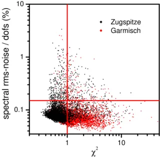
Table 1. Spectral micro windows and molecular line parameters compilations investigated in this study to find an optimum retrieval strategy.
spectral micro windows molecular line parameters compilations (MW)
MW1 2613.70–2615.40 HITRAN 2000 (HIT 00, Rothman et al., 2003)∗ MW2 2650.60–2651.30
MW3 2835.50–2835.80 HITRAN 2004 (HIT 04, Rothman et al., 2005) MW4 2903.60–2904.03
MW5 2921.00–2921.60 HITRAN 2008 (HIT 08, Rothmann et al., 2009)
∗HITRAN 2000 including the official April 2001 update release on CH
4and H2O.
vapor levels typical for NDACC stations. Section 2.8 shows how to calculate column-averaged dry-air mole fractions (XCH4)from the retrieved methane profiles, and Sect. 2.9 gives the final recommendation for the optimum mid-IR re-trieval strategy. The XCH4seasonality is quantified for the Zugspitze site and compared to SCIAMACHY satellite data in Sect. 3. Section 4 gives the summary and an outlook.
2 Retrieval strategy and error characterization
2.1 Goal and approach
A first technical goal in optimizing the retrieval strategy is to investigate how retrievals of vertical profiles of methane can lead to improved precision for total columns compared to a simple scaling of a volume mixing ratio (vmr) profile with an altitude-constant factor. A requirement for such a profile inversion method is that it shall be based upon a ro-bust regularization scheme that can easily be transferred to all NDACC-FTIR stations in a consistent manner. Another strategic goal is to identify a favorable selection out of five mid-IR candidate spectral micro windows (MW, see Table 1) which have been established previously within the EC project UFTIR (http://www.nilu.no/uftir/). Furthermore, we want to find out which of the 3 most recent, official-release HI-TRAN1line parameters compilations (Table 1) is best suited for our mid-infrared micro windows. Finally, a concept for the quality selection of the methane retrievals shall be devel-oped, since this is crucial to obtain a data set with optimum precision.
The conceptual approach is to perform an error charac-terization for multi-annual data sets prepared with varied re-trieval strategies, i.e. varied subsets of the 5 candidate micro windows, and using the 3 different recent HITRAN versions for each case. A focus is on H2O/HDO-CH4interference er-rors which turned out in the course of our study to be the dominant errors in mid-IR methane retrievals which are not carefully optimized (up to≈4 %, for some HITRAN versions
1HIgh-resolutionTRANsmission molecular absorption database
Table 2. Test sites of this study and corresponding range of inte-grated water vapor according to National Center for Environmental Prediction data selected for clear-sky days (FTIR measurement con-ditions).
Wollongong Garmisch Zugspitze (34◦S, (47◦N, (47◦N, 30 m a.s.l.) 743 m a.s.l.) 2964 m a.s.l.) max H2O column (mm∗) 44.9 34.9 12.7 mean H2O column (mm) 17.9 14.9 3.3
min H2O column (mm) 6.9 1.9 0.2
∗1 mm corresponds to 3.345×1021cm−2.
and micro-windows, see Table 4 below). Since the magni-tude of the H2O/HDO-CH4interference errors is expected to depend also on the overall humidity level, all test runs will be performed for data from the 3 different NDACC-FTIR sites Wollongong, Garmisch, and Zugspitze in parallel. As Ta-ble 2 shows, these test sites cover humidity levels between extremely wet to very dry due to their differing climatic lo-cations. This range of integrated water vapor is representa-tive for the clear-sky measurement conditions of the whole NDACC FTIR network.
2.2 FTIR measurements at 3 test sites
2.2.1 Zugspitze FTIR system
The Zugspitze (47.42◦N, 10.98◦E, 2964 m a.s.l.) solar FTIR system was set up in 1995 as part of the “Alpine Station” of the NDACC network. It is operated by the Group “Variabil-ity and Trends” at IMK-IFU2, Karlsruhe Institute of Tech-nology, together with a variety of additional sounding sys-tems at the Zugspitze site3. These include an AERI (Atmo-spheric Emitted Radiance Interferometer), GPS (Global Po-sitioning System for water vapor soundings), and two water vapor lidars (both a differential absorption lidar and a Ra-man lidar). The FTIR team contributes to satellite validation and studies of atmospheric variability and trends (e.g. mann and Buchwitz, 2005; Sussmann et al., 2005a,b; Suss-mann and Borsdorff, 2007; SussSuss-mann et al., 2009; Vogel-mann et al., 2011). The FTIR system is based upon a Bruker IFS 125/HR interferometer; details can be found in Suss-mann and Sch¨afer (1997). The interferograms used for the methane retrievals have been recorded with an InSb detector using an optical path difference of typically 175 cm, averag-ing a number of 6 scans (≈7-min integration time).
2Institute for Meteorology and Climate Research – Atmospheric Environmental Research, http://www.imk-ifu.kit.edu/atmospheric variability.php
2.2.2 Garmisch FTIR system
The Garmisch solar FTIR system (47.48◦N, 11.06◦E, 743 m a.s.l) was set up in 2004 and is part of the TCCON network operating in the near-infrared for high-precision re-trieval of column-averaged mixing ratios of carbon dioxide and methane. The system performs mid-IR NDACC-type measurements in parallel (in alternating mode on the time scale of several minutes). The latter are utilized for this study. The system is operated together with a variety of addi-tional sounding systems by IMK-IFU at the Garmisch site4, which comprises, e.g. an NDACC aerosol lidar, GPS, and an ozone lidar. The Garmisch FTIR data contribute to satellite validation and studies of atmospheric variability and trends (e.g. Morino et al., 2011; Borsdorff and Sussmann, 2009). The FTIR system is similar to the mid-IR Zugspitze set up with additional InGaAs and Si diodes (dual recording) for the near-IR measurements plus high-precision solar track-ing (Bruker A547N,±2 min of arc) and high-accuracy
pres-sure meapres-surement devices. The meapres-surement settings for the Garmisch mid-IR methane measurements are the same as de-tailed for the Zugspitze above.
2.2.3 Wollongong FTIR system
The Wollongong solar FTIR system (34.45◦S, 150.88◦E, 35 m a.s.l.) is operated by the University of Wollongong’s Center for Atmospheric Chemistry. It was setup in 1995 as part of the NDACC network. The instrument installed in 1995 was a Bomem DA8 FTIR system which operated from 1995 to 2007 (described in Griffith et al., 1998). During 2007 a Bruker IFS 125/HR instrument replaced the Bomem DA8 as part of an upgrade of the FTIR measurement program to expand the measurement capability to both the mid-IR and near-IR (Jones et al., 2011; Wunch et al., 2011). For this pa-per only the Bruker data were used. Spectra used for the CH4 retrievals were obtained from interferograms recorded from an InSb detector, and a KBr beamsplitter or a CaF2 beam-splitter. The optical path difference was 257 cm, coadding 2 consecutive interferograms giving an integration time of approximately 4 min.
2.3 Spectral information and interfering species
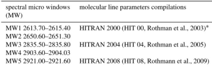
The spectral contributions from methane and all relevant in-terfering species to our candidate spectral micro windows within the measured solar absorption spectrum are plotted in Fig. 1. The most important interfering species, i.e. water vapor and its isotope HDO, can vary by factors>200 be-tween dry NDACC sites like Zugspitze and humid sites like Wollongong, see Table 2. The spectral effect from this huge dynamic range is demonstrated in Fig. 1, see dashed versus solid lines. This provides evidence that it is important for 4Garmisch site details can be found at http://www.imk-ifu.kit. edu/315.php
Table 3.Interfering species that have to be taken into account in the 5 candidate micro windows (MW, defined in Table 1).
MW interfering species fit (scaling)
MW 1 HDO, CO2 MW 2 HDO, CO2
MW 3 HDO
MW 4 HDO, H2O, NO2 MW 5 HDO, H2O, NO2
moderate to high humidity levels to include joint fitting of HDO in all micro windows as well as joint fitting of H2O in MW 4 and MW 5 (Table 3). Failing to perform this joint fit-ting of H2O/HDO may lead to H2O/HDO-CH4interference errors of the order of≈4 %. This can easily be verified from
plotting the ratio of a methane column time series retrieved with and without this joint fitting as a function of HDO col-umn level. This approach is detailed in Sect. 2.7.3 below. Another approach has been followed by von Clarmann and Echle (1998) and Dudhia et al. (2002), where a minimization of interference errors was achieved without joint fitting of interfering species. This was performed by extensive micro window cutting, aiming to minimize the inclusion of spectral signatures of interfering species while preserving the main features of the target species.
2.4 Spectroscopic line data and spectral fitting residuals
Figure 2 shows the spectral residuals (measured minus cal-culated) averaged over more than one year of solar absorp-tion measurements analyzed by the non-linear least squares spectral fitting software SFIT2 (Pougatchev et al., 1995), version 3.94. The spectral residuals indicate systematic er-rors in the spectroscopic line data. Intriguingly, the quality of HITRAN line parameters in our 5 candidate spectral mi-cro windows has degraded with the two updates from HI-TRAN 2000 (including the April 2001 update release for CH4and H2O) to HITRAN 2004, and from HITRAN 2004 to HITRAN 2008. Figure 2a shows three major effects (numbers for the root-mean square of the residuals are given within the figure):
i. HITRAN 2000 is the spectroscopy compilation with the overall smallest residuals.
solar
CO
2
NO
2
H2O
HDO CH
4
total
2650.6 2650.8 2651.0 2651.2
0.7 0.8 0.9 1.0 1.1 1.2
MW 2
2835.5 2835.6 2835.7 2835.8
0.8 0.9 1.0 1.1
n
o
rm
a
li
z
e
d
i
n
te
n
s
it
y
wave number (cm-1)
MW 3
2614.0 2614.5 2615.0
0.6 0.7 0.8 0.9 1.0 1.1 1.2
n
o
rm
a
li
z
e
d
i
n
te
n
s
it
y
wave number (cm-1)
MW 1
2903.6 2903.7 2903.8 2903.9 2904.0
0.4 0.5 0.6 0.7 0.8 0.9 1.0 1.1 1.2 1.3
MW 4
2921.0 2921.2 2921.4 2921.6
0.2 0.4 0.6 0.8 1.0 1.2 1.4 1.6 1.8
n
o
rm
a
li
z
e
d
i
n
te
n
s
it
y
wave number (cm-1)
MW 5
Fig. 1. Spectral contribution plot for a solar zenith angle of 65◦. Solid lines are for a H2O column of 44.9 mm (Wollongong maximum); dashed lines correspond to a H2O column of 0.2 mm (Zugspitze minimum).
verified by comparing the residuals to the contribution plots (Fig. 1).
iii. HITRAN 2008 shows similar problems as HI-TRAN 2004 for the non-methane line parameters. Ad-ditionally, the residuals due to methane have increased with HITRAN 2008. In particular, a huge error in the line strength of the 2921.33 cm−1methane line was in-troduced.
Figure 2b proves that HITRAN 2000 behaves comparably well for all three test sites in spite of their strongly differing humidity levels.
2.5 Profile retrieval optimizing precision for columns
2614.0 2614.5 2615.0 -1.5
-1.0 -0.50.0 0.5 1.0 1.5
2650.6 2650.8 2651.0 2651.2
-1.5 -1.0 -0.50.0 0.5 1.0 1.5
2835.5 2835.6 2835.7
-1.5 -1.0 -0.5 0.0 0.5 1.0 1.5
2903.6 2903.7 2903.8 2903.9 -1.5
-1.0 -0.5 0.0 0.5 1.0 1.5
2921.0 2921.2 2921.4
-1.5 -1.0 -0.50.0 0.5 1.0 1.5
2614.0 2614.5 2615.0
2835.5 2835.6 2835.7 2835.8
2903.6 2903.7 2903.8 2903.9 2904.0
2921.0 2921.2 2921.4 2921.6
2650.6 2650.8 2651.0 2651.2
rms (%) = 0.13, 0.27,0.41
rms (%) = 0.11, 0.13,0.27
rms (%) = 0.13, 0.10,0.17
rms (%) = 0.11, 0.13,0.22
MW 1
rms (%) = 0.09,0.11, 0.09
HIT00 (Garmisch) HIT04 (Garmisch)
a)
HIT08 (Garmisch)MW 4 MW 3 MW 2
s
p
e
c
tr
a
l
re
s
id
u
a
ls
(
%
)
MW 5
wave number (cm
-1)
rms (%) = 0.10, 0.13,0.06
rms (%) = 0.05, 0.11,0.09
rms (%) = 0.07, 0.13,0.11
rms (%) = 0.06, 0.11,0.10
rms (%) = 0.04, 0.09,0.07
Wollongong (HIT00) Garmisch (HIT00)
b)
Zugspitze (HIT00)Fig. 2. (a)Averaged residuals (measured minus calculated) for the station Garmisch using HITRAN 2000 versus HITRAN 2004, and HITRAN 2008.(b)Averaged residuals using HITRAN 2000 shown for the 3 different stations Wollongong, Garmisch, and Zugspitze.
IRWG5, and is thereby easily transferable to all ground-based FTIR stations of the NDACC network.
The classical approach to retrieve total columns from ground-based FTIR spectrometry has used least squares spectral fitting with iterative scaling of an volume mixing ratio (vmr) a priori profile via one (unconstrained) altitude constant factor. This had been implemented in non-linear least squares spectral fitting software like SFIT1 (e.g. Rins-land et al., 1984) or GFIT (e.g. Toon et al., 1992). Because of the free profile scaling, this approach has the advantage that it does not damp true scaling-type columns variability in the retrieval. However, it frequently leads to significant spectral residuals. This is because of (i) likely discrepancies of the shape of the true profile relative to the a priori pro-file (e.g. caused by variability of the tropopause altitude) and (ii) possible spectral line shape errors in the forward calcula-tion and/or the measurement. Both effects can introduce sig-nificant biases to the retrieved columns. A strategy to reduce
5InfraredWorkingGroup
this problem is to derive total columns from profile retrievals which helps to better integrate the area of the measured ab-sorption line shape and thereby obtain a more accurate esti-mate of the total column integral.
Therefore, we favor a more robust retrieval that combines the advantages of both a profile scaling and a profiling ap-proach while avoiding their disadvantages at the same time. For this purpose, we construct a regularization matrix that allows for some (constrained) flexibility in profile shape (de-gree of flexibility to be tuned) and also guarantees that pure profile-scaling type variations remain unconstrained. This can be achieved as follows.
The forward model F maps the profiles to be retrieved from state spacexinto measurement spacey. The retrieval is the (ill-posed) inverse mapping fromy toxwhich is formu-lated as a least squares problem. Due to the non-linearity of
F, a Newtonian iteration is applied and a regularization term
R∈Rn×n(inverse model withnlayers) is used that allows one to constrain the solution and thereby avoid oscillating profiles
xi+1 = xi +
KTx,iS−1ε Kx,i +R
−1
(1)
× nKTx,iS−1ε [y −F(xi)] −R(xi −xa)
o
,
where the subscriptidenotes the iteration index andxais the a priori profile. HereKx=F/∂xare the Jacobians andSεis the measurement covariance (assumed to be diagonal with a signal-to-rms-noise ratio of 500 in our formulation). Using first order Tikhonov regularization (Tikhonov, 1963),Ris set up by the relation
R = αLT1 L1 ∈ Rn×n, (2)
whereαis the regularization strength andL1is the discrete first derivative operator
L1 =
−1 1 0 ··· 0
0 −1 1 . .. ... ..
. . .. . .. . .. 0 0 ··· 0 −1 1
∈ R(n−1)×n, (3)
which constrainsxin a way such that a constant profile is fa-vored for the differencex−xa. The priorxafor methane and the interfering species (including H2O) was constructed from a multi-annual average output from the Whole Atmosphere Chemistry Climate Model (WACCM, Garcia et al., 2007), and from the US Standard Atmosphere for species which were not available from WACCM (e.g. HDO). Pressure-temperature profiles have been obtained from NCEP (Na-tional Center for Environmental Prediction).
Tests have shown that it is a good choice to apply the TikhonovL1regularization to percentage changes (or scal-ing factors) of the vmr of the individual profile layers to be retrieved. Another choice would be the application ofRto the state vector given in units of absolute vmr, which implies a differing altitude dependency of the regularization strength. An argument for the implementation ofL1 in units of per-centage profile changes is that this leads to the limiting case
of a vmr-profile scaling, in case the regularization strengthα
is tuned towards infinity leading to 1 degree of freedom for signal (dofs, see Rodgers, 2000 for a definition): vmr-profile scaling is one of the best-tested retrieval approaches and well known to yield very robust retrieval results for total columns. The details of the retrieval grid chosen impact the altitude dependency of the regularization strength. For an constant retrieval grid Eqs. (2) and (3) result in an altitude-constant regularization strength. This turned out to work ro-bustly for water vapor (Sussmann et al., 2009) as well as for the methane retrievals and other species. In order to preserve this altitude-constant regularization in case a non-altitude constant retrieval grid is used, a transformationT
has to be applied to Eq. (2), i.e.
R′ = αLT1 T L1, (4)
where
T =
1
1z21 0 ··· 0
0 1
1z22
. .. ...
..
. . .. . .. 0
0 ··· 0 1
z2n−1
∈ R(n−1)×(n−1), (5)
and1zi is the vertical thickness of a layer with indexiof the non-equidistant retrieval grid.
Finally, the regularization strengthαcan be optimized in a way to achieve minimum diurnal variation (optimum pre-cision) of the retrieved CH4 columns. Figure 3a shows the L-curve, and Fig. 3b its second derivative which shows an optimum for anαcorresponding to dofs≈2. Figure 3c shows
that at the same time one gets a dofs≈2, a minimum for the
diurnal variation is obtained (0.23 %, 1σ). This is nearly a factor of 2 lower than the diurnal variation of 0.39 % which is obtained in case a simple vmr-profile scaling approach is used (dofs≡1, see point on the very left hand side of Fig. 3c). Together with the L-curve this provides evidence that the op-timized Tikhonov profile retrieval accounts for true profile variations in a way that helps to better integrate the mea-sured absorption-line profile, i.e. that is closer to an equiv-alent width retrieval than a simple vmr-profile scaling ap-proach. See Appendix A for ensembles of retrieved profiles and total-column averaging kernels.
2.6 Quality selection
Final quality selection of the methane retrievals is crucial, e.g. for obtaining a data set of methane columns with best possible precision. Any quality selection is a trade off be-tween improving the overall quality of the data and losing too much data. Therefore, we present an approach that opti-mizes this problem for ground-based FTIR spectrometry.
7 6 5 4 3 2 1 0.2
0.3 0.4 0.5 0.00 0.01 0.02 0.14 0.16 0.18 0.20 0.22
log(α)
dofs =3.0
5
dofs =4.3
8
dofs =2.3
6
dofs =1.9
4 dofs
=1.5 3
d
iu
rn
a
l
va
ri
a
ti
o
n
(
%
)
dofs =1.0
4
2
n
d d
e
ri
v.
l
o
g
(
χ
2 )
c) b)
lo
g
(
χ
2 )
a)
Fig. 3. Optimizing regularization strengthαof TikhonovL1 re-trievals of CH4(using a diagonal measurement covariance with a signal-to-rms-noise ratio of 500) via a test ensemble of all Garmisch year 2007 measurements. (a)Mean L-curve, i.e. goodness of fit (χ2) of as a function ofα. The residual term withinχ2is the over-all rms-residual from the spectral fit and the noise term withinχ2is calculated from the wave number interval 2615.25–2615.40 cm−1. (b)Second derivative (curvature) of the L-curve. (c)Mean diurnal variation (1σ) as a function ofα. Corresponding numbers for the information content (dofs) are indicated.
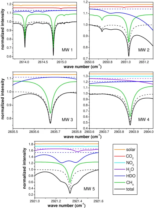
spectra with bad quality. To remove these we added another quality selection threshold for spectral rms-noise divided by the information content (dofs) as outlined in Fig. 4. The rea-son for using the spectral rms-noise to dofs ratio is as fol-lows. Figure 5a (upper trace) shows that the time series of spectral noise contains a seasonal cycle with a maximum in winter (minimum in summer) which is due to the changing solar zenith angle. This means that a classical quality crite-rion using a simple threshold for the rms-noise would elim-inate more measurements in winter than in summer. How-ever, Fig. 5a (lower trace) indicates that the dofs shows a seasonal cycle with same phase. This is a result of the ab-sorption line depth changing with varying solar zenith an-gle in such a way that during winter there is higher dofs, as the lines are deeper. Deeper lines from (winter) spectra with higher noise level (less sun light than during summer) can be analyzed at a comparable quality (retrieval noise) level as the weaker lines from summer spectra, which show a lower
1 10
0.1 1 10
Zugspitze Garmisch
s
p
e
c
tr
a
l
rm
s
-n
o
is
e
/
d
o
fs
(
%
)
χ
2Fig. 4.Quality selection criteria and thresholds for goodness of fit (χ2) and spectral quality (rms-noise) relative to information content (dofs). Data points are for 5 years of measurements.
average noise level. Thus, an optimized quality criterion can be utilized using a threshold for the ratio of the spectral rms-noise and dofs, see Fig. 5b. Another advantage is that this threshold is more generic as it is no longer sensitive to the average zenith angle of a specific site. Therefore the same threshold can be used for sites at differing geographic loca-tions. We used one common quality threshold of 0.15 % (red line in Fig. 5b) for all three test sites. In addition, to remove a few obvious outliers, we added a threshold for the devia-tion of an individual methane-column measurement from the daily mean of<1.8 %.
2.7 Micro-window characterization and interference-error analysis
2.7.1 Information content
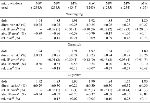
Table 4 (first rows) shows that MW 5 is the most important micro window within the set of 5 candidate MWs: excluding MW 5 leads to a stronger drop of dofs than excluding any of the other MWs. E.g. there is a drop of dofs from 1.94 to 1.75 as a result of dropping micro window 5 for Wollongong.
2.7.2 Diurnal variation
The precision of the retrieved CH4columns (mostly limited by the impact of clouds) is estimated from the 1-σ diurnal variation of retrievals from single spectra (derived from av-erage of several scans,≈4–7-min integration), averaged over
0.10 0.15 0.20 0.25 0.30 0.35 0.40
2006 2007 2008 2009 2010 2011 1.4
1.6 1.8 2.0 2.2
2006 2007 2008 2009 2010 2011 0.0
0.5 1.0 1.5 2.0
rm
s
-n
o
is
e
/
d
o
fs
(
%
)
b)
rm
s
-n
o
is
e
(
%
)
a)
d
o
fs
Fig. 5. (a)Upper trace: time series of spectral rms-noise calculated from the out-of-band 2615.25–2615.40 cm−1wave number interval for the Zugspitze site; lower trace: resulting degrees of freedom for signal (dofs) from fitting micro windows 1, 3, and 5 using HITRAN 2000. (b)Ratio of spectral residuals and dofs. Red line: quality selection threshold.
the precision of remote sounding column measurements of CH4. In reality, part of the diurnal variation will be caused by real variations in CH4over the day. Therefore this method gives an upper limit for the precision (see, e.g. Warneke et al., 2006). Table 4 (second rows) shows that an average precision of 0.25 % is achieved for Wollongong, 0.23 % for Garmisch, and 0.29 % for Zugspitze using all 5 candidate micro win-dows. Furthermore, the table shows that dropping individ-ual micro windows leads to a slight increase of the diurnal variation, related to the corresponding drop in dofs. Using HITRAN 2004 or HITRAN 2008 instead of HITRAN 2000 also leads to a slight but significant increase of the diurnal variation (Table 5). In order to minimize interference errors, our final recommendation will be to use only micro windows 1, 3, and 5 together with HITRAN 2000 (HIT00 MW (135) strategy)). The resulting diurnal variations are 0.27 % for Wollongong, 0.26 % for Garmisch, and 0.30 % for Zugspitze (Table 4).
One note on the HIT08 MW (1234) strategy. This strat-egy might be favored by the “esthetic” reason that it com-prises latest version HITRAN. However, it will be shown in Sect. 2.7.3 that this strategy causes significantly higher in-terference errors than our recommended HIT00 MW (135) strategy comprising HITRAN 2000. Table 6 shows two further disadvantages of using HIT08 MW (1234): for Garmisch (Wollongong) there is an increased di-urnal variation of ±0.28 (±0.31) compared to using
the HIT00 MW (135) strategy which leads to ±0.26
(±0.27). Also the information content is lower using HIT08 MW (1234), namely 1.75, compared to 1.80 attain-able by using HIT00 MW (135).
This means that a precision of <0.3 % is attainable for total column methane from mid-IR NDACC-type measure-ments and this is comparable to the TCCON state of the art for methane of<0.3 % for single spectra. However, two points have to be considered for a more detailed quantitative comparison:
i. The integration time for one single TCCON spectrum is about 1.6 min while the integration time of the mid-IR NDACC measurements of our study is ≈4–7 min.
Recalculating the TCCON precision for a 7-min in-tegration would lead to ≈0.3 %/sqrt (7/1.6) = 0.14 %
which would be a factor of≈2 better than the mid-IR
precision of<0.3 % for total column methane.
ii. However, in case of the mid-IR retrievals no correction for variability induced by clouds is performed, while the TCCON retrievals use a normalization by simulta-neous O2 column measurements (Washenfelder et al., 2003; Wunch et al., 2011). The TCCON retrievals ad-ditionally include a correction for solar intensity fluctu-ations via the DC signal of the interferograms accord-ing to Keppel-Aleks et al. (2007). Both measures lead to a reduction of the diurnal variation (caused, e.g. by clouds), but they are applied only in case of the TC-CON measurements, not in case of the mid-IR NDACC measurements.
Therefore, our interpretation of the relatively good mid-IR precision (only factor≈2 lower compared to TCCON) is that
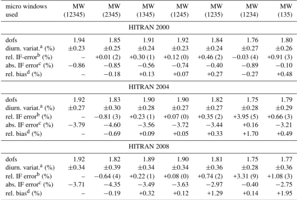
Table 4. Effect of dropping individual micro windows using data from 3 test sites with strongly differing humidity levels; impact on information content (dofs), interference errors, and diurnal variation. The HITRAN 2000 line parameters compilation was used.
micro windows MW MW MW MW MW MW MW
used (12345) (2345) (1345) (1245) (1235) (1234) (135)
Wollongong
dofs 1.94 1.85 1.91 1.92 1.83 1.75 1.80
diurn. variat.a(%) ±0.25 ±0.25 ±0.25 ±0.25 ±0.26 ±0.28 ±0.27 rel. IF errorb(%) – −0.07 (1) +0.31 (1) +0.10 (0) +0.72 (2) −0.17 (3) +1.20 (3) abs. IF errorc(%) −0.89 −0.96 −0.58 −0.79 −0.17 −1.06 +0.14
rel. biasd(%) – −0.15 +0.21 +0.09 +0.39 −0.43 +0.73
Garmisch
dofs 1.94 1.85 1.91 1.92 1.84 1.76 1.80
diurn. variat.a(%) ±0.23 ±0.25 ±0.24 ±0.23 ±0.24 ±0.27 ±0.26 rel. IF-errorb(%) - +0.01 (2) +0.30 (1) +0.12 (0) +0.46 (2) −0.03 (4) +0.91 (3) abs. IF errorc(%) −0.86 −0.85 −0.56 −0.74 −0.40 −0.89 −0.10
rel. biasd(%) – −0.18 +0.13 +0.07 +0.27 −0.27 +0.48
Zugspitze
dofs 1.92 1.83 1.90 1.90 1.84 1.75 1.80
diurn. variat.a(%) ±0.29 ±0.30 ±0.29 ±0.30 ±0.30 ±0.32 ±0.30 rel. IF errorb(%) – −0.03 (1) +0.11 (1) +0.02 (1) +0.25 (1) −0.01 (4) +0.41 (2) abs. IF errorc(%) −0.34 −0.37 −0.23 −0.32 −0.09 −0.35 +0.02
rel. biasd(%) – −0.17 +0.02 +0.05 +0.10 −0.23 +0.14
aDiurnal variation of individual days (1σ), averaged over all days of full time series. b“Relative interference error”, defined as HDO/H
2O-CH4interference error relative to
MW (12345), see Fig. 8; uncertainties in brackets are for 95 % confidence.c“Absolute interference error”, defined as the negative of the sum over the rel. IF errors (row above).
dBias rel. to MW (12345), see Fig. 8.
(Figs. 4 and 5) help to bring the mid-IR columnar methane retrievals’ precision to this unexpected high quality level.
2.7.3 Interference errors
In the recent paper by Sussmann and Borsdorff (2007) we introduced a general formulation for a class of “interference errors” which could not be described by any of the classi-cal four error categories of remote sounding (e.g. Rodgers, 2000, Eq. 3.16); i.e. errors in the retrieval of a target species (e.g. methane) as a result from the smoothing effect from interfering species (e.g. HDO). Additional interference ef-fects can be due to errors in forward model parameters of the interfering species (e.g. erroneous HITRAN parameters for HDO) which can be propagated into the retrieval of the target species (e.g. methane). The latter class of errors can be de-scribed by the existing concept of “(forward) model param-eter errors” (second term in Rodgers, 2000, Eq. 3.16). We will hereafter present an empirical interference error analysis and, in doing so, a separation of these two differing classes of errors is neither needed nor possible. Therefore, we will use the term “interference errors” in this paper to designate either or both of the two interference phenomena.
Figure 6 shows the ratio of Garmisch year-2007 methane time series derived with two differing retrieval strategies, i.e. (i) the retrieval strategy HIT08 MW (12345) using all 5 candidate micro windows and HITRAN 2008 line param-eters (which was the starting point of our study), and (ii) the retrieval strategy HIT00 MW (135) using HITRAN 2000 and using only micro windows 1, 3, and 5, which will be the final recommendation resulting from our study. The ratio time se-ries shows a significant seasonal discrepancy between these two retrieval strategies.
The reason for this seasonal discrepancy can be under-stood from Fig. 7 which shows the same ratio as above as a function of the HDO column level (also for the other test sites). The HDO columns were taken from the joint HDO re-trieval of the HIT00 MW (135) run. Occurrence of a strong HDO-CH4interference error for all test sites (up to≈5 % for
Table 5. Effect from dropping individual micro windows using 3 different HITRAN versions for the test station Garmisch; impact on information content (dofs), interference errors, and diurnal variation.
micro windows MW MW MW MW MW MW MW
used (12345) (2345) (1345) (1245) (1235) (1234) (135)
HITRAN 2000
dofs 1.94 1.85 1.91 1.92 1.84 1.76 1.80
diurn. variat.a(%) ±0.23 ±0.25 ±0.24 ±0.23 ±0.24 ±0.27 ±0.26 rel. IF-errorb(%) – +0.01 (2) +0.30 (1) +0.12 (0) +0.46 (2) −0.03 (4) +0.91 (3) abs. IF errorc(%) −0.86 −0.85 −0.56 −0.74 −0.40 −0.89 −0.10
rel. biasd(%) – −0.18 +0.13 +0.07 +0.27 −0.27 +0.48
HITRAN 2004
dofs 1.92 1.83 1.90 1.90 1.82 1.75 1.79
diurn. variat.a(%) ±0.27 ±0.30 ±0.28 ±0.27 ±0.27 ±0.28 ±0.29 rel. IF errorb(%) – −0.81 (3) +0.23 (1) +0.07 (0) +0.35 (2) +3.95 (5) +0.66 (3) abs. IF errorc(%) −3.79 −4.60 −3.56 −3.72 −3.44 +0.16 −3.21
rel. biasd(%) – −0.69 +0.09 +0.05 +0.33 +1.70 +0.49
HITRAN 2008
dofs 1.92 1.82 1.89 1.90 1.81 1.75 1.77
diurn. variat.a(%) ±0.34 ±0.39 ±0.34 ±0.34 ±0.36 ±0.28 ±0.36 rel. IF errorb(%) – −0.64 (4) +0.22 (1) +0.08 (0) +0.74 (2) +3.31 (9) +1.08 (3) abs. IF errorc(%) −3.71 −4.35 −3.49 −3.63 −2.97 −0.40 −2.75
rel. biasd(%) – −0.19 +0.32 +0.12 +1.29 +0.14 +1.95
aDiurnal variation of individual days (1σ), averaged over all days of full time series. b“Relative interference error”, defined as HDO/H
2O-CH4interference error relative to
MW (12345), see Fig. 8; uncertainties in brackets are for 95 % confidence.c“Absolute interference error”, defined as the negative of the sum over the rel. IF errors (row above). dBias rel. to MW (12345), see Fig. 8.
Jan Mar May Jul Sep Nov 0.95
0.96 0.97 0.98 0.99 1.00 1.01 1.02
C
H
4c
o
lu
m
n
s
r
a
ti
o
Garmisch
HIT08 MW(12345) HIT00 MW(135)
Fig. 6.Ratio of one year of Garmisch year 2007-methane retrievals with two differing retrieval strategies, i.e. using all 5 candidate mi-cro windows and HITRAN 2008 (HIT08 MW (12345)) versus us-ing only micro windows number 1, 3, and 5, and HITRAN 2000 (HIT00 MW (135)) plotted as a time series.
We will show in the following that this interference ef-fect is due to the HIT08 MW (12345) retrieval strategy, i.e. this interference effect can practically be eliminated by using the HIT00 MW (135) retrieval strategy. In order to show this we perform a systematic study as indicated in
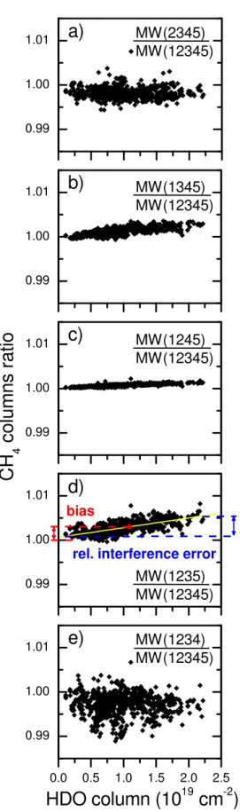
Fig. 8. Using HITRAN 2000 and dropping stepwise each of the 5 candidate micro windows, we quantify the result-ing interference effect relative to the HIT00 MW (12345) reference run: e.g. it can be quantified from Fig. 8d that dropping micro window 4 leads to a total relative interfer-ence error of +0.46 % which is indicated in blue in the fig-ure. Additionally, an overall bias of +0.27 % relative to the 5-micro window run results (indicated in red in Fig. 8d). Note, this overall bias has two major contributions in general, (i) from the average interference error (e.g. dominant con-tribution in Fig. 8d), and/or (ii) from methane line strength errors (e.g. dominant contribution in Fig. 8e).
Table 4 gives numbers for all the relative interference er-rors for all 3 test stations; e.g. for Wollongong there is a significant relative interference error upon dropping MWs 2 and 4 (+0.31 % and +072 %, respectively), while dropping MWs 1, 3 and 5 leads only to minor interference errors of
−0.07 %, +0.10 %, and−0.17 %, respectively. Similar re-sults are obtained for the other test stations (Table 4).
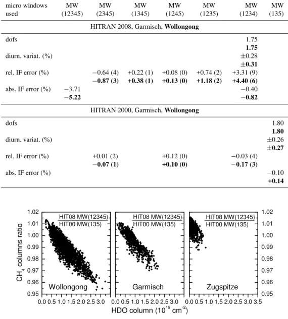
Table 6. Comparison of the HIT08 MW (12345) and HIT08 MW (1234) retrieval strategies versus the recommended strategy HIT00 MW (135). Numbers are for Garmisch (standard font) and Wollongong (bold). Use of HIT08 MW (12345) is out of discussion (Wollongong absolute interference error−5.22 %) but also the use of the HIT08 MW (1234) strategy is strongly discouraged because ofi)
high absolute interference errors (e.g.−0.82 % for Wollongong) and (ii) strong “internal tension” (strong rel. interference error contributions from differing micro windows with opposite sign, e.g.−0.87 % versus +1.18 % for Wollongong).
micro windows MW MW MW MW MW MW MW
used (12345) (2345) (1345) (1245) (1235) (1234) (135)
HITRAN 2008, Garmisch,Wollongong
dofs 1.75
1.75
diurn. variat. (%) ±0.28
±0.31 rel. IF error (%) −0.64 (4) +0.22 (1) +0.08 (0) +0.74 (2) +3.31 (9)
−0.87 (3) +0.38 (1) +0.13 (0) +1.18 (2) +4.40 (6)
abs. IF error (%) −3.71 −0.40
−5.22 −0.82
HITRAN 2000, Garmisch,Wollongong
dofs 1.80
1.80
diurn. variat. (%) ±0.26
±0.27
rel. IF error (%) +0.01 (2) +0.12 (0) −0.03 (4)
−0.07 (1) +0.10 (0) −0.17 (3)
abs. IF error (%) −0.10
+0.14
0.0 0.5 1.0 1.5 2.0 2.5 3.0 0.0 0.5 1.0 1.5 2.0 2.5 3.0 3.5 0.95 0.96 0.97 0.98 0.99 1.00 1.01 1.02 HIT08 MW(12345)
HIT00 MW(135)
HDO column (1019 cm-2) Garmisch
HIT08 MW(12345) HIT00 MW(135)
Zugspitze
0.0 0.5 1.0 1.5 2.0 2.5 3.0 0.95
0.96 0.97 0.98 0.99 1.00 1.01 1.02
HIT08 MW(12345) HIT00 MW(135)
C
H 4
c
o
lu
m
n
s
r
a
ti
o
Wollongong
Fig. 7. Investigation of the seasonal artifact shown in Fig. 6: ratio of about one year of methane retrievals with two differing retrieval strategies as in Fig. 6, now plotted as a function of HDO column level for the 3 test sites (HDO columns are from the joint HDO retrieval of the HIT00 MW (135) run).
use micro windows number 1, 3, and 5, and drop MWs 2 and 4 as long as no better spectroscopy than HITRAN 2000 is available. (It will be shown below that HITRAN 04 and HIT 08 give worse results than HITRAN 2000.)
In the following we characterize the absolute quantity of the interference error of the optimum (HIT00 MW (135)) trieval strategy; e.g. for Garmisch the HIT00 MW (135) re-trieval strategy leads to a relative interference error of +0.91
0.99 1.00 1.01
0.99 1.00 1.01
0.99 1.00 1.01
0.0 0.5 1.0 1.5 2.0 2.5 0.99
1.00 1.01
MW(2345)
MW(12345)
MW(1345)
MW(12345)
a)
b)
MW(1234)
MW(12345)
MW(1235)
MW(12345)
MW(1245)
MW(12345)
C
H
4c
o
lu
m
n
s
r
a
ti
o
c)
0.99 1.00 1.01
bias
rel. interference error
d)
HDO column (10
19cm
-2)
e)
Fig. 8.Ratio of Garmisch year-2007 retrievals of columnar methane with one MW out of 5 dropped(a)–(e) versus retrieval with all 5 MWs plotted as a function of HDO column level. HITRAN 2000 was used in all cases. The definition of total relative interference error and overall bias is indicated.
would be that MWs 2 and 4 would cause an absolute inter-ference error with similar magnitude but opposite sign; i.e., the relative interference error MW (24)/MW (12345) would be around≈ −0.9 %. This is not to be the case: according to
Table 4 the relative interference error MW (24)/MW (12345) for Garmisch is +0.14 (8), i.e. in the order of≈0.1 %. This
means that our starting assumption is erroneous, the abso-lute interference effect of the MW (135) run is only in the order of ≈0.1 % and the observed relative interference
ef-fect of +0.91 % is mainly due to an absolute interference error of the MW (12345) run of ≈ −0.9 %. This
con-clusion can be double checked by assuming the opposite, namely that the MW (135) run is absolute interference free would mean that the MW (12345) run would have an abso-lute interference error of about −0.9 % caused by MWs 2 and 4. This would mean that the relative interference error MW (24)/MW (12345) should be around zero. In reality it is +0.14 (8) % for Garmisch (Table 4), i.e. our assump-tion is valid to a good approximaassump-tion. In other words, the Garmisch HIT00 MW (1235) run is interference free at the
≈0.1 % level.
In continuation of the previous considerations we de-fine a way to calculate an “absolute interference error” of a certain retrieval strategy to be the negative of the sum of the relative interference errors found by dropping the different micro windows that make up this strategy; e.g., the absolute interference error for the HIT00 MW (135) run would be the negative of the sum of the rela-tive interference errors derived from the ratio time se-ries MW (2345)/MW (12345), MW (1245)/MW (12345), and MW (1234)/MW (12345), i.e. the absolute interfer-ence error for the Garmisch HIT00 MW (135) run would be – [(+0.01 %) + (+0.12 %) + (−0.03 %)] =−0.10 % (see Ta-ble 4). In an analogous absolute interference errors have been derived for Wollongong (+0.14 %) and for Zugspitze (+0.2 %). Note the improvement of these MW (135) runs relative to the MW (12345) runs, since the latter show an ab-solute interference error of−0.89 % for Garmisch,−1.96 %
for Wollongong, and−0.35 % for Zugspitze (Table 4).
It is a crucial result (from Table 4) that the quality ranking of the various retrieval strategies, according to the absolute interference error, is the same for our 3 test sites in spite of their strongly differing water vapor levels. This means that it does make sense, indeed, to recommend one joint (optimum) retrieval strategy for all NDACC sites. According to Table 4 this is the HIT00 MW (135) strategy.
However, for a final recommendation we still have to investigate the impact of varied spectroscopy upon inter-ference errors. All hitherto discussed results of this pa-per used HITRAN 2000 (Table 4). Table 5 shows the in-crease of interference errors upon using HITRAN 2004 or HITRAN 2008 instead. Using HITRAN 2004 leads to an unacceptable value for the absolute interference error of
−3.79 % for the MW (12345) run and still−3.21 % for the
seen from the relative interference error of +3.95 % for the HIT04 MW (1234) run. This is clearly a result of the large residual at the left hand side of MW 5 due to HDO with HI-TRAN 2004 (rms of 0.27 %, see Fig. 2a) which is signifi-cantly larger than the residual of 0.13 % with HITRAN 2000 (Fig. 2a). Also a large relative interference error from the HIT04 MW (2345) run of−0.81 % arises which is caused by
increased residuals in MW 1 with HITRAN 2004 compared to the case with HITRAN 2000 (Fig. 2a).
From Table 5 one might wonder whether the HIT04 MW (1234) retrieval strategy would be a reasonable alternative since the absolute interference error is +0.16 %, which is larger, but of the same order of magnitude of the proxy of
−0.10 % for the recommended HIT00 MW (135) retrieval
strategy. However, the relatively small (+0.16 %) abso-lute interference error for the HIT04 MW (1234) run com-prises large relative interference error components with op-posite sign from the individual micro windows. These can-cel out by chance, see Table 5: −0.16 % =−0.81 % (from
MW (2345), i.e. due to MW 1) + 0.23 % (from MW (1345), i.e. due to MW 2) + 0.07 % (from MW (1245), i.e. due to MW 3) + 0.35 % (from MW (1235), i.e. due to MW 4). This means that the HIT04 MW (1234) retrieval strategy contains strong “internal tension”, i.e. retrievals using the individual micro windows alone, would lead to strongly differing re-trieval results. This is not a recommendable, stable rere-trieval approach.
Finally, we investigate the use of HITRAN 2008. Simi-larly to HITRAN 2004, the use of HITRAN 2008 leads to an unacceptably large absolute interference error: it is−3.75 % for the HIT08 MW (12345) run and still −2.75 % for the HIT08 MW (135) run. The major reason for this can be seen from the relative interference error of +3.31 (9) % for the HIT08 MW (1234) run which clearly is a result of the large MW-5 residual due to the CH4line at 2921.33 cm−1 (rms of 0.41 % see Fig. 2a), which is significantly larger than the residual of 0.27 % with HITRAN 2004 and the residual of 0.13 % with HITRAN 2000 (Fig. 2a).
Just for completeness, the HIT08 MW (1234) retrieval strategy is no alternative, since the absolute interference error for it is −0.40 % for Garmisch (Table 5) which is
significantly larger than the value of −0.10 % achieved
with our recommended HIT00 MW (135) retrieval strat-egy (for Garmisch). In addition, Table 5 shows that the HIT04 MW (1234) run also comprises large relative interfer-ence error components with opposite sign from the individual micro windows (−0.64 %, +0.22 %, +0.08 %, +0.74 % for MWs 1–4, respectively). This means the HIT08 MW (1234) retrieval strategy also contains strong “internal tension” – similar to what has been found for the HIT04 MW (1234) strategy.
These numbers show that the HIT00 MW (135) strat-egy is favorable over the HIT08 MW (1234) stratstrat-egy for the medium-humidity site Garmisch. We expect that the disadvantages of the HIT08 MW (1234) strategy become
even more pronounced for the wettest site Wollongong. To show this we calculated analogous numbers for Wollongong, see Table 6. Indeed, the absolute interference error of the HIT08 MW (1234) strategy approaches the unacceptable 1 % level for Wollongong (−0.82 %). Also the “internal tension”
is even higher compared to Garmisch with a strong negative interference error contribution from MW 1 (−0.87(3) %) and
a strong positive contribution from MW 4 (+1.18(2) %), see Table 6.
To conclude this section, we validate our concept of calculating absolute interference errors. We give 4 validation examples. First, we derived for Garmisch from the HIT00 MW (135) strategy an absolute in-terference error of −0.10 % (Table 6), and for the
HIT08 MW (12345) strategy an absolute interference er-ror of −3.71 % (Table 6). If we combine this in-formation we would expect a relative interference error for HIT08 MW (12345)/HIT00 (MW135) of −3.71 %– (−0.10 %) =−3.61 %. This agrees with the relative
interfer-ence error, which we can independently derive directly from Fig. 7, i.e. MW (12345)/HIT00 (MW135) =−3.71 (7) %,
with a discrepancy of +0.10 %. The second exam-ple is the analogous exercise for Wollongong: here we derived for the HIT00 MW (135) strategy an absolute interference error of +0.14 % (Table 6), and for the HIT08 MW (12345) strategy −5.22 % (Table 6). If we
combine this information we would expect a relative in-terference error for HIT08 MW (12345)/HIT00 (MW135) of −5.22 %−0.14 % =−5.36 %. This agrees with the
relative interference error which we derive from Fig. 7, i.e. MW (12345)/HIT00 (MW135) =−5.58 (6) %, with a discrepancy of +0.22 %. The third validation ex-ample is again for Garmisch; i.e. combining the abso-lute interference errors for the HIT00 MW (135) strat-egy with the HIT08 MW (1234) stratstrat-egy (Table 6), where we would expect a relative interference error for HIT08 MW (1234)/HIT00 (MW135) of −0.40 %–
(−0.10 %) =−0.3 %. This agrees with the relative
in-terference error which we derive directly from Fig. 9, i.e. HIT08 MW (1234)/HIT00 (MW135) =−0.51(4) % with
a discrepancy of +0.21 %. The fourth validation example is the analogous case for Wollongong. Again from the abso-lute interference errors (Table 6) the expectation for the rel-ative HIT08 MW (1234)/HIT00 (MW135) interference error can be derived (−0.82 %–0.14 % =−0.96 %), and this agrees with the direct determination from Fig. 9 (−1.16 (4) %) with a discrepancy of +0.20 %.
All validation results are summarized in Table 7. The overall validation result is that our method of absolute in-terference error estimation yields results with an accuracy at the ≈0.2 % level or better. This confirms the validity
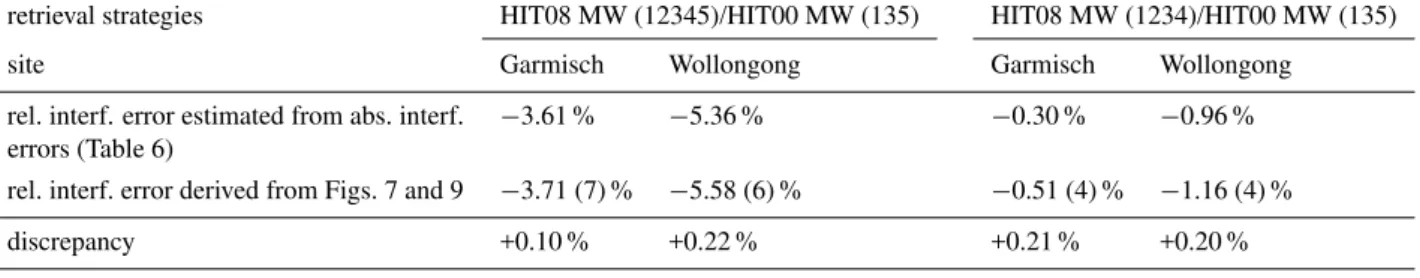
Table 7. Four validation cases using two independent ways of estimating relative interference errors. The discrepancy is a measure for the accuracy of the method of estimating absolute interference errors. For details see text.
retrieval strategies HIT08 MW (12345)/HIT00 MW (135) HIT08 MW (1234)/HIT00 MW (135)
site Garmisch Wollongong Garmisch Wollongong
rel. interf. error estimated from abs. interf. −3.61 % −5.36 % −0.30 % −0.96 % errors (Table 6)
rel. interf. error derived from Figs. 7 and 9 −3.71 (7) % −5.58 (6) % −0.51 (4) % −1.16 (4) %
discrepancy +0.10 % +0.22 % +0.21 % +0.20 %
0.0 0.5 1.0 1.5 2.0 2.5 0.97 0.98 0.99 1.00 1.01 1.02
0.0 0.5 1.0 1.5 2.0 2.5 3.0 0.97
0.98 0.99 1.00 1.01 1.02
HDO column (1019 cm-2)
Garmisch
HIT08 (1234) HIT00 (135) HIT08 (1234)
HIT00 (135)
C
H 4
co
lu
m
n
s
ra
ti
o
Wollongong
Fig. 9. Ratio plots showing significant relative HDO-CH4interference errors which are dominated by the unfavorable HIT08 MW (1234) retrieval strategy while the recommended HIT00 MW (135) retrieval strategy is practically interference free (see Sect. 2.7.3).
errors (Tables 4–6) is significant. In particular, we conclude that within this 0.2 % uncertainty the HIT00 MW (135) re-trieval strategy (absolute interference error +0.14 % for Wol-longong,−0.10 % for Garmisch) is to be favored over the
HIT08 MW (1234) retrieval strategy (absolute interference error−0.86 % for Wollongong,−0.4 % for Garmisch). 2.8 Calculation of column-averaged dry-air mole
fractions
The retrieved individual methane total columns were divided by dry air columns to obtain column-averaged dry-air mole fractions of methane (XCH4). Dry air columns were cal-culated using NCEP pressure-temperature-humidity (PTU) profiles by calculating the total air column from the PT pro-files and substracting water vapor columns obtained from in-tegrating the NCEP water vapor profiles. Not all NDACC sites perform quality controlled surface pressure measure-ments as TCCON sites do. Therefore we investigated the quality of NCEP pressure information and its interpolation to an elevated site. For this purpose we performed a multi-year
comparison of NCEP-derived pressure for the Garmisch sta-tion (743 m a.s.l.) versus the TCCON pressure sensor (1-min values from a high-quality pressure transducer which is regularly quality checked against a mercury barometer). We found a bias of−0.21 hPa with a standard deviation of
1.6 hPa. NCEP PTU profiles are available four times a day (06:00, 12:00, 18:00, 24:00 GMT) and were interpolated to the time of the FTIR measurement. This is recommended because of the strong diurnal cycle of water vapor columns above most sites.
Table 8.Optimum strategy for retrieval of methane from mid-infrared solar spectra designated as MIR-GBM v1.0.
micro windows (interfering species fitted) 2613.70–2615.40 (HDO, CO2) 2835.50–2835.80 (HDO)
2921.00–2921.60 (HDO, H2O, NO2)
line list HITRAN 2000 including 2001 update release
retrieval constraint TikhonovL1
regularization strength αoptimized via L-curve/minimum diurnal altitude dependency of reg. strength variation (dofs≈2)
a priori vmr profiles altitude constant on per-cent-vmr scale
background fit WACCM
linear slope
retrieval quality selection threshold (1.0) forχ2,
threshold (0.15 %) for rms-noise/dofs
calculation of column-averaged dry-air use 4-times-daily-NCEP PTU profiles, mole fractions interpolate to FTIR measurement time,
calculate air column, substract water vapor column
for a harmonized NDACC retrieval strategy of methane. The FTIR retrievals of integrated water vapor used in Fig. 10 have been performed with the retrieval strategy of Sussmann et al. (2009) and have recently been inter-compared against differential absorption lidar measurements showing excellent agreement (Vogelmann et al., 2011).
2.9 Recommended retrieval strategy MIR-GBM v1.0
We make the point that it does make sense to recommend one joint mid-IR retrieval strategy for all NDACC sites. Our conclusion is based upon two findings; (i) the outcome from Sect. 2.7 that the quality ranking of the 24 differing retrieval strategies (using differing micro windows and HITRAN ver-sions) according to the absolute H2O/HDO-CH4interference error is the same for all three test sites of our study. (ii) The 3 test sites cover strongly differing levels of integrated wa-ter vapor which are representative of the whole NDACC net-work. This means we could not find any indication that there could be a retrieval strategy, optimized for the highest-humidity NDACC sites that would not also be the optimum for the driest sites.
The outcome from Sect. 2.7 (Tables 4 and 5) is that the optimum strategy for all sites is using HITRAN 2000 and micro windows 1, 3, and 5 (HIT00 MW (135)). This se-lection, together with our inverse method (Sect. 2.5) and the scheme for quality selection (Sect. 2.6) as well as the scheme for calculating column-averaged dry-air mole frac-tions (Sect. 2.8) comprises our new strategy for mid-IR ground-based methane retrievals. We refer to it as MIR-GBM v1.0 thereafter, see Table 8 for its definition. Table 9 gives our overall quality estimates. In another, ongoing study we perform an inter-calibration of MIR-GBM v1.0 XCH4to
Table 9. Information on accuracy and precision for methane column-averaged dry-air mole fractions retrieved from mid-infrared solar spectra with the retrieval strategy MIR-GBM v1.0.
precision (1-σ diurnal variation)∗ <0.3 % seasonal bias (H2O/HDO-interference error) <0.14 %
∗for 7-min integration
TCCON measurements. This will be subject of an upcoming publication.
3 Seasonality and comparison to SCIAMACHY data
0 2 4 6 8 10 12 0
2 4 6 8 10 12
"
"
# ! & $"!$ & #$%
Fig. 10. Intercomparison of integrated water vapor (IWV) above the Zugspitze retrieved from the solar FTIR with the strategy of Sussmann et al. (2009) versus integrated water vapor profiles from NCEP. Four-times-daily NCEP profiles were interpolated to the times of the FTIR measurements.
et al., 2008a,b; Schneising et al., 2009, 2011) and it is of in-terest to see what the current state of the art is compared to our ground-based retrieval MIR-GBM v1.0.
Figure 11 shows the de-trended seasonality of XCH4 de-rived from the Zugspitze time series. From the full Zugspitze time series covering 1995-2011 we have taken into account only the time interval between the beginning of 2004 up to the end of 2009 [2004, 2009] covering the period for which SCIAMACHY data are available. Red points in Fig. 11 are Zugspitze multi-annual monthly means for this time span. Underlying individual-year monthly means are based on 42 individual FTIR measurements on average. Since methane has shown a renewed increase during 2007–2009 after a near zero-trend period before (Rigby et al., 2008; Dlu-gokencky et al., 2009; Frankenberg et al., 2011; Schneising et al., 2011) we performed a linear de-trending for the period [2007, 2009] before calculating the multi-annual monthly means from the full [2004, 2009] interval. The de-trending was performed by the approach described in Gardiner et al. (2008).
An intra-annual function (2nd order Fourier series) was fitted to the de-trended multi-annual monthly means (red line in Fig. 11). The seasonal amplitude is 16.3±2.9 ppb
or 1.0±0.2 %. The phase of the seasonality can be
char-acterized by an approximate minus-sine-type behavior with a minimum in March/April and a maximum in September. The maxima are somewhat broader and the minima narrower than a simple sine function, however, and are described by the Fourier coefficients of Table 10 more quantitatively.
-2.0
-1.5
-1.0
-0.5
0.0
0.5
1.0
1.5
2.0
Jan Mar May Jul Sep Nov
-40 -30 -20 -10 0 10 20 30 40
d
e-tre
nd
ed
X
C
H4
a
no
m
al
y
(%
)
SCIA 04/05 SCIA all
de
-tr
en
de
d
X
C
H4
a
no
m
al
y
(p
pb
)
Zugspitze FTIR 2nd ord. Fourier Zugspitze FTIR 04/05
Fig. 11. Red points: multi-annual mean seasonality of column-averaged dry-air mole fractions of methane retrieved from Zugspitze FTIR. It has been derived from the de-trended monthly-mean time series in the interval [2004, 2009] with the retrieval strat-egy MIR-GBM v.1.0 (Table 10). Error bars are standard errors of the multi-annual monthly means for 95 % confidence. Red line: Fit of a 2nd order Fourier series. Grey squares: Same as red points but using only [2004, 2005] FTIR data. Grey line: Seasonality de-rived from SCIAMACHY WFMDv2.0 data taken from Fig. 12 of Schneising et al. (2011) for the [2004, 2009] time interval. Black line: same as grey line but using only SCIAMACHY [2004, 2005] data.
Table 10. Parameters describing the seasonality of column-averaged mole fractions of methane.
amplitudea phase Fourier componentsb Zugspitze FTIRc
47◦N, 11◦E 16.2±2.9 ppbd min: March/April a1=−4.5 ppb or 0.94±0.17 % max: Sep a2=−15.8 ppb
“minus-sine type” a3= 2.7 ppb a4=−0.4 ppb SCIAMACHYe
NH 13.7±2.6 – –
30◦N–90◦N 12.4±8.0 ppb – –
aDefined as (max-min)/2 of 2nd order Fourier fit to multi-annual monthly means
of de-trended time series, see Fig. 11. bDescribing the fitted intra-annual function
a1cos (2π t) +a2sin (2π t) +a3cos (4π t) +a4sin (4π t), see Fig. 11. c Retrieved
with MIR-GBM v1.0, defined in Table 8. d Error for amplitude calculated from
combining the standard errors (σ/sqrt(n))for the minimum (using March and April individual-year monthly means) and the maximum (August–October monthly means).
eRetrieved with WFMD v2.0, numbers taken from Schneising et al. (2011, Table 3
therein).
Northern Hemisphere, see, e.g. Fig. 12 in Schneising et al. (2009). The reason for the much more FTIR compatible phase of the WFMD v2.0 retrievals relative to WFMD v1.0 is probably due to the use of improved methane and water vapor spectroscopy (Frankenberg et al., 2008a,b) and/or the use of an updated Carbon Tracker version (to correct the re-trieved methane mole fractions for CO2seasonal variability), see Sect. 3.2 in Schneising et al. (2011) for a detailed discus-sion of the latter improvements.
4 Summary and outlook
4.1 Summary
We have developed a strategy for retrieval of atmospheric methane from mid-infrared solar absorption spectra with minimized seasonal bias<0.14 % and optimized precision
<0.3 % (1-σ diurnal variation, 7-min integration). This opti-mum strategy is designated as MIR-GBM v1.0.
If other, non-optimum micro window selections and/or spectroscopy selections are used, dominant systematic errors up to≈5 % arise which are due to interference by water vapor and HDO. Because of this finding, our study was performed in parallel with data from 3 FTIR sites (Zugspitze, Garmisch, and Wollongong) located in differing climatic zones with strongly differing mean levels of precipitable water ranging from 0.2 mm to 44.9 mm for clear sky conditions. This spans the range of the humidity levels of all NDACC sites. We de-rived a concept for empirical estimation of the absolute inter-ference error of a certain retrieval strategy. Performing a sys-tematic study with 24 different retrieval strategies (8 different
micro window selections and 3 different HITRAN versions) we found that the quality ranking of these 24 strategies with respect to the absolute interference error is the same for all three test sites. (Precision is only weakly impacted by the retrieval strategy). This means that it does make sense, in-deed, to agree upon one joint mid-IR retrieval strategy for all NDACC sites.
The cornerstones of the recommended retrieval strategy MIR-GBM v1.0 have been summarized in Table 8. The best available spectroscopy for the mid-infrared methane re-trievals is currently HITRAN 2000 including the 2001 update release. Intriguingly, HITRAN 2004 and HITRAN 2008 lead to worse spectral residuals in our 5 candidate spectral micro windows. These spectral residuals are due to line parame-ter errors for methane, HDO, and H2O. However, even using HITRAN 2000, only 3 of the candidate micro windows are suitable for a retrieval (first, third, fifth, if indexed for in-creasing wave number). The other two micro windows (sec-ond and fourth) lead to significant H2O/HDO-CH4 interfer-ence errors up to several per cent. For some retrieval strate-gies with moderate overall interference errors strong “inter-nal tension” is observed; i.e. there are significant interference errors due to the individual micro windows, with opposite sign. These cancel out partly in the combined multi-window retrieval. In these cases strongly differing retrieval results from stand-alone retrievals with the individual micro win-dows are observed. Examples of such non-recommendable retrieval strategies are those using the first 4 micro windows together with HITRAN 2004 or 2008.