Abstract
The convergence characteristic of the conventional two-noded Euler-Bernoulli piezoelectric beam finite element depends on the configuration of the beam cross-section. The element shows slower convergence for the asymmetric material distribution in the beam cross-section due to material-loc’ing caused by extension-bending coupling. Hence, the use of conventional Euler-Bernoulli beam finite element to analyze piezoelectric beams which are generally made of the host layer with asymmetrically surface bonded piezoe-lectric layers/patches, leads to increased computational effort to yield converged results. Here, an efficient coupled polynomial interpolation scheme is proposed to improve the convergence of the Euler-Bernoulli piezoelectric beam finite elements, by eliminat-ing ill-effects of material-lockeliminat-ing. The equilibrium equations, de-rived using a variational formulation, are used to establish rela-tionships between field variables. These relations are used to find a coupled quadratic polynomial for axial displacement, having contributions from an assumed cubic polynomial for transverse displacement and assumed linear polynomials for layerwise electric potentials. A set of coupled shape functions derived using these polynomials efficiently handles extension-bending and electrome-chanical couplings at the field interpolation level itself in a varia-tionally consistent manner, without increasing the number of nodal degrees of freedom. The comparison of results obtained from numerical simulation of test problems shows that the conver-gence characteristic of the proposed element is insensitive to the material configuration of the beam cross-section.
Keywords
Coupled field, finite elements, piezoelectric, smart structure.
An Efficient Coupled Polynomial Interpolation Scheme
to Eliminate Material-locking in the Euler-Bernoulli
Piezoelectric Beam Finite Element
Litesh N. Sulbhewar a P. Raveendranathb
Department of Aerospace Engineering, Indian Institute of Space Science and Technology, Thiruvananthapuram, India. a Research Scholar
[email protected] b Adjunct Professor [email protected]
http://dx.doi.org/10.1590/1679-78251401 Received 10.06.2014
Latin American Journal of Solids and Structures 12 (2015) 153-172 1 INTRODUCTION
The piezoelectric smart structures have dominated the current state of the art shape and vibra-tion control technology due to their high reliability (Crawley and de Luis, 1987). Electromechani-cal coupling present in the piezoelectric materials adds the ability to respond to the subjected forced environment. Piezoelectric beams render a wide class of smart structures (Benjeddou et al., 1997). Their numerical analysis plays an important role in the design of piezoelectric beam based control systems. The analysis of piezoelectric beam requires efficient and accurate modeling of both mechanical and electric responses (Sulbhewar and Raveendranath, 2014 a; Zhou et al., 2005).
As most of the smart beams are thin (Marinkovic and Marinkovic, 2012), Euler-Bernoulli beam theory has been favored by many researchers for their formulations. Analytical models based on the Euler-Bernoulli theory were presented by Crawley and de Luis (1987), Crawley and Anderson (1990) and Abramovich and Pletner (1997) for static and dynamic analyses of piezoe-lectric beams. Crawley and de Luis (1987) carried out the parametric studies to show the effec-tiveness of piezoelectric actuators in transmitting the strain to the substrate. Crawley and Ander-son (1990) extended this analysis to establish the range over which the simpler analytical solu-tions are valid. Abramovich and Pletner (1997) proposed closed form solusolu-tions for induced curva-ture and axial strain of an adaptive sandwich struccurva-ture.
Also, the classical laminate theory based piezoelectric plate finite elements (Hwang and Park, 1993; Lam et al., 1997; Wang et al., 1997) and beam elements (Balamurugan and Narayanan, 2002; Bendary et al., 2010; Bruent et al., 2001; Carpenter, 1997; Gaudenzi et al., 2000; Hanagud et al., 1992; Kumar and Narayanan, 2008; Manjunath and Bandyopadhyay, 2004; Robbins and Reddy, 1991; Sadilek and Zemcik, 2010; Stavroulakis et al., 2005; Zemcik and Sadilek, 2007) are available in the literature for the analysis of extension mode piezoelectric beams.
A four-noded classical plate bending element with an elemental electric potential degree of freedom was used by Hwang and Park (1993) for the vibration control analysis of composite plates with piezoelectric sensors and actuators, while with nodal electric potential degrees of free-dom for static shape control study by Wang et al. (1997). Lam et al. (1997) developed a four-noded classical plate finite element with negative velocity feedback control to study the active dynamic response of integrated structures.
Latin American Journal of Solids and Structures 12 (2015) 153-172 (2010) carried out the static and dynamic analyses of composite beams with piezoelectric materi-als using a classical laminate theory based beam element with layerwise linear through-thickness distribution of nodal electric potential.
Generally, the Euler-Bernoulli theory based beam elements give good convergence of finite el-ement results (Reddy, 1997). However, when the beam cross-section consists of asymmetrical ma-terial distribution, these elements suffer from material-locking due to presence of
extension-bending coupling (Raveendranath et al., 2000). As most of the piezoelectric beam structures
con-tain a piezoelectric material layer asymmetrically bonded to the host structure, it activates the extension-bending coupling and hence deteriorates the finite element convergence. One of the ways to get rid of material-locking is the use of a higher-order polynomial interpolation for the axial displacement along the length of the beam (Raveendranath et al., 2000; Sulbhewar and Raveendranath, 2014b). A more efficient way to remove ill-effects of material-locking is the use of coupled polynomial field interpolations which incorporate the extension-bending coupling in an appropriate manner, without increasing nodal degrees of freedom (Raveendranath et al., 2000; Sulbhewar and Raveendranath, 2014 c; 2014 d). For Euler-Bernoulli piezoelectric beam finite element, electromechanical coupling also has to be accommodated properly along with the exten-sion-bending coupling in a coupled polynomial field based formulation.
Here in this study, a novel interpolation scheme, based on coupled polynomials derived from governing equilibrium equations, is proposed to eliminate material-locking in the Euler-Bernoulli piezoelectric beam finite element. The variational formulation is used to derive governing equilib-rium equations which are used to establish the relationship between field variables. The polyno-mial derived here for the axial displacement field for the beam contains an additional coupled term along with conventional linear terms, having contributions from an assumed cubic polyno-mial for transverse displacement and assumed linear polynopolyno-mials for layerwise electric potential. This coupled term facilitates the use of higher order polynomial for axial displacement without introducing any additional generalized degrees of freedom in the formulation. A set of coupled shape functions is obtained from these coupled field polynomials which accommodates extension-bending and piezoelectric couplings in a variationally consistent manner. The accuracy of the present formulation is shown by comparing results with those from ANSYS 2D simulation and conventional formulations. Convergence studies are carried out to prove the efficiency of the pre-sent Euler-Bernoulli piezoelectric beam formulation with coupled shape functions over the con-ventional formulations with assumed independent shape functions.
2 THEORETICAL FORMULATION
Latin American Journal of Solids and Structures 12 (2015) 153-172
among them. The top and bottom faces of the piezoelectric layers are fully covered with electro-des. Mechanical and electrical quantities are assumed to be small enough to apply linear theories of elasticity and piezoelectricity.
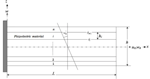
Figure 1: Geometry of a general multilayered piezoelectric smart beam.
2.1 Mechanical Displacements and Strain
The Euler-Bernoulli theory is used for which the field expressions are given as (Bendary et al., 2010):
'
0 0
( , ) ( ) ( )
u x z u x zw x (1)
0
( , ) ( )
w x z w x (2)
where u x z( , )and w x z( , )are the displacements in the longitudinal and transverse directions of the beam, respectively. u x0( )and w x0( )are the centroidal axial and transverse displacements,
respec-tively. ( ) 'denotes derivative with respect to x. DimensionsL b h, , denote the length, width and the total thickness of the beam, respectively.
Axial strain field is derived using usual strain-displacement relation as:
' ''
0 0
( , )
( , ) ( ) ( )
x
u x z
x z u x zw x
x
(3)
2.2 Electric Potential and Electric Field
The through-thickness profile of the electric potential ( , )x z in a piezoelectric layer is taken as linear (Bendary et al., 2010). As shown in Figure 1, the two dimensional electric potential takes the values of i1( )x and i( )x at the top and bottom faces of the
th
i piezoelectric layer, respective-ly. The electric field in the transverse direction (Ez) can be derived from electric potential as
Latin American Journal of Solids and Structures 12 (2015) 153-172
( , ) ( )
( , )
i i i
z
i
x z x
E x z
z h
(4)
where i i1i, is the difference of potentials at the top and bottom faces of the th
i piezoelec-tric layer with thickness hi.
3 REDUCED CONSTITUTIVE RELATIONS
The smart beam consisting layers of conventional/composite/piezoelectric material with isotropic or specially orthotropic properties is considered here. It has axes of material symmetry parallel to beam axes, in which electric field is applied in the transverse direction. For extension mode beam, the transversely poled piezoelectric material is subjected to the transverse electric field. The elas-tic, piezoelectric and dielectric constants are denoted by C eij, kj( ,i j1...6)andk(k1, 2,3), respec-tively. The constitutive relations for such a system are given as (Sulbhewar and Raveendranath, 2014 c): 31 11 31 3 i k k x x i i i i z z e Q E e D
(5)
where (i=1….number of piezoelectric layers), (
k
=1…..total number of layers in beam). The con-stants Q e, and denote elastic (N m2), piezoelectric (C m2 ) and dielectric (F m) properties reduced for the beam geometry (Sulbhewar and Raveendranath, 2014 c).4 VARIATIONAL FORMULATION
Hamilton s principle is used to formulate the piezoelectric smart beam. It is expressed as (Sulbhewar and Raveendranath, 2014 c):
2 2
1 1
( ) ( ) 0
t t
t t
K H W dt K H W dt
(6)where, K=kinetic energy, H =electric enthalpy density function for piezoelectric material and mechanical strain energy for the linear elastic material and W =external work done.
4.1 Electromechanical and Strain Energy Variations
For the th
j conventional/composite material layer, the mechanical strain energy variation is given as:
j j
j x x
V
H dV
(7)Latin American Journal of Solids and Structures 12 (2015) 153-172
i i i i
i x x z z
V
H E D dV
(8)Substituting values of axial strain (x), electric field (
i z
E ) form equations (3), (4) and using them along with constitutive relations given by equation (5) in expressions (7) and (8); the total varia-tion on the potential energy of the smart beam is given as:
2 2 1 1 ' ' ''0 11 0 0 11 1 0 31 0
' '' ' ''
11 1 0 11 2 0 31 0 0 31 1 0
'' 0
2
31 1 3 0 ( )
t t
k k k k i i
i i
t t x
k k k k i i i i
i i
i
i i i i
i i i i
H dt u Q I u Q I w e I h
Q I u Q I w e I h u e I h w
w dx dt
e I h I h
(9)where (i=1….number of piezoelectric layers), (
k
=1…..total number of layers in beam) and4.2 Variation of Kinetic Energy
Total kinetic energy of the beam is given as (Sulbhewar and Raveendranath, 2014 c):
1 2 2 1 2 k k z k x zK b
u w dz dx
(10)where
k is volumic mass density of kthlayer in 3kgm and (k =1…total number of layers in the
beam). Substituting values of uand w from equations (1) and (2) and applying variation, to de-rive at:
2 2 1 1 ' ' '0 0 0 1 0 0 1 0 2 0 0 0 0
t t
k k k k k
k
t t x
K dt u I u I w w I u I w w I w dx dt
(11)where ( ). denotes t.
4.3 Variation of Work of External Forces
Total virtual work of the structure can be defined as the product of virtual displacements with forces for the mechanical work and the product of the virtual electric potential with the charges for the electrical work. The variation of total work done by external mechanical and electrical loading is given by (Sulbhewar and Raveendranath, 2014 c):
2 2
1 1 0
V V S S
u w u w
t t V S C C u w t t S
uf wf dV uf wf dS
W dt dt
uf wf q dS
(12)1 1
1
( q q ) ( 1).
k
q k k
Latin American Journal of Solids and Structures 12 (2015) 153-172 in which fV,fS,fC are volume, surface and point forces, respectively. q0and S are the charge
density and area on which charge is applied.
5 DERIVATION OF COUPLED FIELD RELATIONS
The relationship between field variables is established here using static governing equations. For static conditions without any external loading, the variational principle given in equation (6) reduc-es to (Sulbhewar and Raveendranath, 2014 c):
0 H
(13)
Applying variation to the basic variables in equation (9), the static governing equations are ob-tained as:
''
'''
'0: 11 0 0 11 1 0 31 0 0
k k k k i i
i i
u Q I u Q I w e I h
(14)
'''
''''
''0: 11 1 0 11 2 0 31 1 0
k k k k i i
i i
w Q I u Q I w e I h
(15)
From equation (14), we can write the relationship of axial displacement (u0) with transverse
dis-placement ( w0) and electric potential () as:
'' ''' ' 0 1 0 2
u ui
i
u w (16)
where 1 ( 11 1) / ( 11 0)
u k k k k
Q I Q I
and 2 ( 31 0 ) / ( 11 0)
ui i i k k
i
e I h Q I
. The constantsmu (m1, 2)which relate the field variables are the functions of geometric and material properties of the beam. This rela-tion is used in the next secrela-tion to derive coupled field polynomials.
6 FINITE ELEMENT FORMULATION
Using the variational formulation described above, a finite element model has been developed here. The model consists of two mechanical variables (u0and w0) and layerwise electrical variables (i)
where (i1…..number of piezoelectric layers in the beam). In terms of natural coordinate, a cubic
polynomial for transverse displacement (w0) and linear polynomials for iare assumed as given in
equations 17 (a) and 17 (b), respectively. The transformation between and global coordinate x
along the length of the beam is given as
2(xx1) / (x2x1) 1 with (x2x1)l, being the lengthof the beam element.
2 3
0 0 1 2 3
w b bb b (17a)
0 1
i i
i c c
(17b
)
Using these polynomials for w0and iin equation (16) and integrating with respect to , we get
Latin American Journal of Solids and Structures 12 (2015) 153-172
20 6 1 / 3 2 / 4 1 1 0
u ui i
u l b l c aa (18)
It is noteworthy that equation (18) contains a quadratic term in addition to the conventional linear terms. The formulation which use linear interpolation for u0(Bendary et al., 2010) is known
to exhibit material-locking when applied to beams with asymmetric cross-section (Sulbhewar and Raveendranath, 2014 b). A higher-order interpolation for u0 as given in equation (18), is expected
to relieve material-locking and improve the rate of convergence (Sulbhewar and Raveendranath, 2014 b). It takes care of extension-bending and electromechanical couplings in a variationally consistent manner with the help of the coupled quadratic term which has contributions from transverse displacement and layerwise electric potential. The 1
utakes care of the bending effects,
while 2uitakes care of electromechanical effects on the axial displacement. As seen from
equa-tions (17) and (18), while employing a quadratic polynomial for interpolation of axial displace-ment, the generalized degrees of freedom are efficiently maintained the same as of the conven-tional formulation of Bendary et al. (2010).
Using equations (17) and (18), the coupled shape functions in equation (19) are derived by usual method. 1 0 1 0 '1 0
0 1 2 3 4 5 6 7 8
1
0 1 2 3 4
' ' ' ' ' 2
0 1 2 3 4 0
2
1 2 0
'2 0 2 0 0 0 0 0 0 0 0
0 0 0 0 0 0
u
u u
u ui u ui
u
w
w w w
i
w w w w
i i i i u w w
u N N N N N N N N
w N N N N
w N N N N u
N N w
w (19)
The expressions for these shape functions in the natural coordinate system are given as:
2 2 2
1 1 2
1 2 3 4
2 2 2
1 1 2
5 6 7 8
2 3 2 2 3 2
1 2 3 4
' 1
3 3
(1 )
; ( 1); ( 1); (1 );
2 2 4 8
3 3
(1 )
; (1 ); ( 1); ( 1);
2 2 4 8
1 1
( 3) ; ( 1); (3 ) ; ( 1);
4 2 8 4 2 8
3 2
u u ui
u u u ui
u u ui
u u u ui
w w w w
w
l
N N N N
l
l
N N N N
l
l l
N N N N
N l
2 ' ' 2 '
2 3 4
1 2
3 1 3 3 1
( 1); 1 ; (1 ); 1 ;
2 2 4 2 2 2 4
1 1
; .
2 2
w w w
i i
N N N
l
N N
(20)
Latin American Journal of Solids and Structures 12 (2015) 153-172
0
0 0
uu u
u
K K
U U F
M
Q
K K
(21)
where M is the mass matrix,
K
uu,
K
u,
K
u,
K
are global stiffness sub-matrices. U,are the glob-al nodglob-al mechanicglob-al displacement and electric potentiglob-al degrees of freedom vectors, respectively. F and Qare global nodal mechanical and electrical force vectors, respectively. Now the general for-mulation has been converted to matrix equation which can be solved according to electrical condi-tions (open/closed circuit), configuration (actuator/sensor) and type of analysis (static/dynamic).7 NUMERICAL EXAMPLES AND DISCUSSIONS
The developed formulation is tested here for the accuracy and efficiency to predict the structural behaviour of piezoelectric extension mode smart beams. The formulation is validated for static (actuator/sensor configuration) and modal analyses. The present Euler-Bernoulli smart beam formulation which uses coupled polynomial based interpolation (hereafter designated as EB-CPI) is compared for performance against conventional Euler-Bernoulli smart beam formulations with assumed independent polynomial based interpolation as used by Bendary et al. (2010) (designated hereafter as EB-IPI).
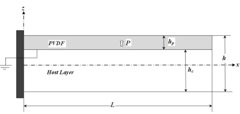
The particular test problem chosen here is the host layer made up of aluminum or 0/90 graphite-epoxy composite material with surface bonded piezoelectric PVDF material layer as shown in Figure 2. The material and geometric properties of the beam are:
Aluminum (Bendary et al., 2010): 3
68.9 ; 0.25; 2769
E GPa kgm .
Graphite-epoxy (Beheshti-Aval and Lezgy-Nazargah, 2013):
(E E GL, T, LT,GTT)(181,10.3,7.17, 2.87)GPa ( LT, TT)(0.28,0.33);1578kgm3.
PVDF (Sun and Huang, 2000): 2 9 1
31 3
2 ; 0.29; 0.046 ; 0.1062 10
E Gpa e Cm Fm
3
1800kgm
4 ; 1 ; 100
c p
h mm h mm L mm.
Latin American Journal of Solids and Structures 12 (2015) 153-172
The set of reference values is obtained from the numerical simulation of test problems with the ANSYS 2D simulation, for which a mesh of PLANE 183 element for host layer with size 100 8 and a mesh of PLANE 223 element for piezoelectric layer with size 100 2 is used.
7.1 Static Analysis: Sensor Configuration
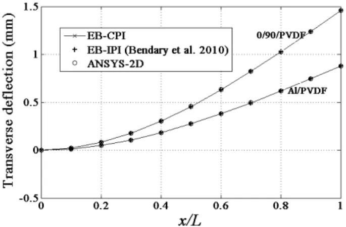
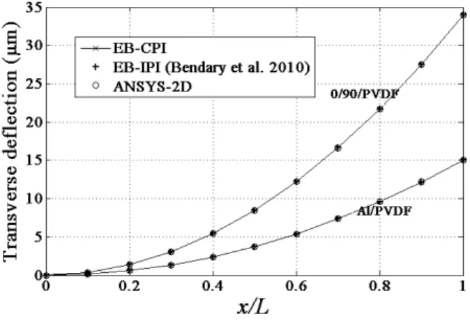
For sensor configuration, the piezoelectric smart cantilever shown in Figure 2 is subjected to a tip load of 1000N. The structural response of the beam is evaluated by present EB-CPI, convention-al EB-IPI of Bendary et convention-al. (2010) and ANSYS 2D simulation. The variations of transverse and axial deflections and potential developed across the piezoelectric layer along the length of the 0/90/PVDF and Al/PVDF beams are plotted in Figures 3, 4 and 5, respectively. As seen from the plots, EB-CPI gives accurate predictions as of EB-IPI of Bendary et al. (2010) and ANSYS 2D simulation. The through-thickness variations of axial stresses developed at the roots of the 0/90/PVDF and Al/PVDF beams are plotted in Figure 6, which validate the use of present cou-pled polynomial interpolation for calculation of derived quantities also.
Figure 3: Sensor configuration: Variation of the transverse deflection along the length of the piezoelectric smart cantilever subjected to a tip load of 1000 N.
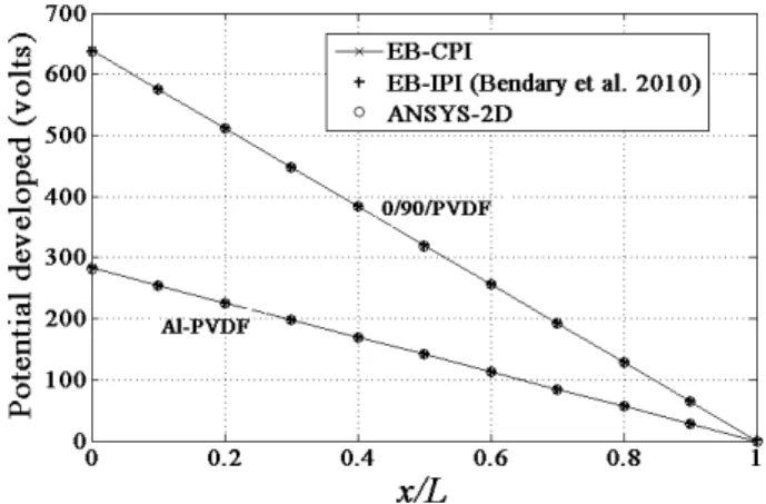
Latin American Journal of Solids and Structures 12 (2015) 153-172 Figure 5: Sensor configuration: Variation of the potential developed across the piezoelectric
layer along the length of the piezoelectric smart cantilever subjected to a tip load of 1000 N.
(a) 0/90/PVDF
(b) Al/PVDF
Latin American Journal of Solids and Structures 12 (2015) 153-172
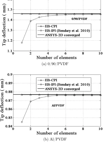
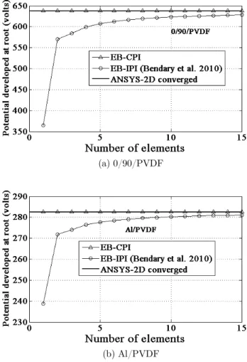
Now the efficiency of the present coupled polynomial based interpolation scheme over the conven-tional independent polynomial based interpolation is proved by the convergence graphs plotted in Figures 7 and 8 for tip deflection and potential developed at the root of the beam, respectively. As seen from the graphs, EB-IPI of Bendary et al. (2010) exhibit material-locking and takes a large number of elements to converge to the accurate predictions as given by 2D simulation. The present EB-CPI is free from material-locking effects and shows single element convergence. This improvement in the performance can be attributed to the coupled term present in the description of the axial displacement given by equation (18). The performance of the conventional formula-tion (Bendary et al., 2010) may be improved by using an assumed independent quadratic interpo-lation for the axial displacement; however it will increase the number of elemental degrees of freedom and computational efforts.
(a) 0/90/PVDF
(b) Al/PVDF
Latin American Journal of Solids and Structures 12 (2015) 153-172 (a) 0/90/PVDF
(b) Al/PVDF
Figure 8: Sensor configuration: Convergence characteristics of the Euler-Bernoulli based piezoelectric beam finite elements to predict the potential developed across the piezoelectric
layer at the root of the piezoelectric smart cantilever subjected to a tip load of 1000 N.
7.2 Static Analysis: Actuator Configuration
Latin American Journal of Solids and Structures 12 (2015) 153-172
Figure 9: Actuator configuration: Variation of the transverse deflection along the length of the piezoelectric smart cantilever actuated by 10 KV.
Figure 10: Actuator configuration: Variation of the axial deflection along the length of the piezoelectric smart cantilever actuated by 10 KV.
Latin American Journal of Solids and Structures 12 (2015) 153-172 (b) Al/PVDF
Figure 11: Actuator configuration: Through-thickness variation of axial stresses developed in the piezoelectric smart cantilever actuated by 10 KV.
7.3 Modal Analysis
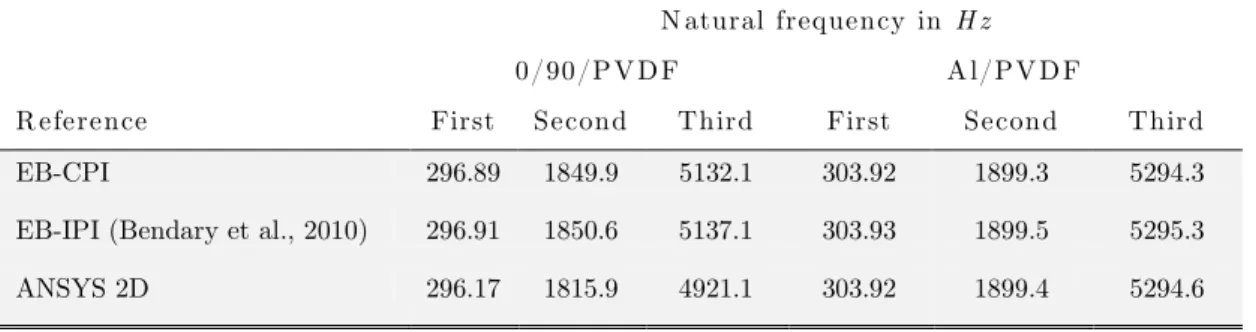
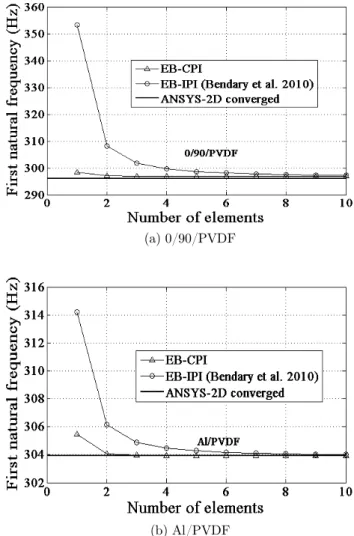
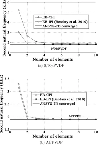
The present EB-CPI is tested here for the accuracy and efficiency to predict the natural frequen-cies of the piezoelectric smart cantilever shown in Figure 2. The converged values of first three natural frequencies of the 0/90/PVDF and Al/PVDF beams evaluated by EB-CPI, EB-IPI of Bendary et al. (2010) and ANSYS 2D simulation are tabulated in Table 1. As seen from the re-sults, EB-CPI gives the accurate predictions for the natural frequencies as predicted by 2D simu-lation and EB-IPI. This validates the use of consistent mass matrices generated by the present coupled polynomial field based interpolation scheme.
N atural frequency in H z 0/90/P V D F A l/PV D F
R eference First Second Third First Second Third EB-CPI 296.89 1849.9 5132.1 303.92 1899.3 5294.3 EB-IPI (Bendary et al., 2010) 296.91 1850.6 5137.1 303.93 1899.5 5295.3 ANSYS 2D 296.17 1815.9 4921.1 303.92 1899.4 5294.6
Latin American Journal of Solids and Structures 12 (2015) 153-172 (a) 0/90/PVDF
(b) Al/PVDF
Figure 12: Modal analysis: Convergence characteristics of the Euler-Bernoulli based piezoelectric beam finite ele-ments to predict the first natural frequency of the piezoelectric smart cantilever.
Latin American Journal of Solids and Structures 12 (2015) 153-172 (a) 0/90/PVDF
(b) Al/PVDF
Figure 13: Modal analysis: Convergence characteristics of the Euler-Bernoulli based piezoelectric beam finite elements to predict the second natural frequency of the piezoelectric smart cantilever.
Latin American Journal of Solids and Structures 12 (2015) 153-172 (b) Al/PVDF
Figure 14: Modal analysis: Convergence characteristics of the Euler-Bernoulli based piezoelectric beam finite elements to predict the third natural frequency of the piezoelectric smart cantilever.
Figure 15: Natural bending modes of the 0/90/PVDF piezoelectric smart cantilever.
8 CONCLUSION
Latin American Journal of Solids and Structures 12 (2015) 153-172
The present formulation gives accurate predictions of finite element results in both static (sensing/actuation) and modal analyses as given by conventional formulation and 2D finite ele-ment simulation, which validate the use of present coupled polynomial field based interpolation.
The present interpolation scheme is free from any locking effect unlike conventional indepen-dent polynomial based interpolation which suffers from material-locking. The convergence studies carried out prove the merit of the present coupled polynomial based interpolation over the con-ventional independent polynomial based interpolations.
The present formulation proves to be the most efficient way to model piezoelectric smart beam with Euler-Bernoulli beam theory.
References
Abramovich, H., Pletner, B. (1997). Actuation and sensing of piezolaminated sandwich type structures, Composite Structures 38: 17-27.
Balamurugan, V., Narayanan, S. (2002). Active vibration control of piezolaminated smart beams, Defence Science J. 51: 103-114.
Beheshti-Aval, S.B., Lezgy-Nazargah, M. (2013). Coupled refined layerwise theory for dynamic free and forced response of piezoelectric laminated composite and sandwich beams, Meccanica, 48: 1479-1500.
Bendary, I.M., Elshafei, M.A., Riad, A.M. (2010). Finite element model of smart beams with distributed piezo-electric actuators,J. Intelligent Material Systems and Structures 21: 747-758.
Benjeddou, A., Trindade, M.A., Ohayon, R. (1997). A unified beam finite element model for extension and shear piezoelectric actuation mechanisms, J. Intelligent Material Systems and Structures 8: 1012-1025.
Bruant, I., Coffignal, G., Lene, F., Verge, M. (2001). Active control of beam structures with piezoelectric actua-tors and sensors: modeling and simulation, Smart Materials and Structures 10: 404-408.
Carpenter, M.J. (1997). Using energy methods to derive beam finite elements incorporating piezoelectric mate-rials, J. Intelligent Material Systems and Structures 8: 26-40.
Crawley, E.F., de Luis, J. (1987). Use of piezoelectric actuators as elements of intelligent structures, AIAA J. 25: 1373-1385.
Crawley, E.F., Anderson, E.H. (1990). Detailed models of piezoceramic actuation of beams, J. Intelligent Material Systems and Structures 1: 4-25.
Gaudenzi, P., Carbonaro, R., Benzi, E. (2000). Control of beam vibrations by means of piezoelectric devices: theory and experiments, Composite Structures 50: 373-379.
Hanagud, S., Obal, M.W., Calise, A.J. (1992). Optimal vibration control by the use of piezoceramic sensors and actuators, J. Guidance, Control, and Dynamics 15: 1199-1206.
Hwang, W.S., Park, H.C. (1993). Finite element modeling of piezoelectric sensors and actuators, AIAA J. 31: 930-937.
Kumar, K.R., Narayanan, S. (2008). Active vibration control of beams with optimal placement of piezoelectric sensor/actuator pairs, Smart Materials and Structures 17: 55008-55022.
Lam, K.Y., Peng, X.Q., Liu, G.R., Reddy, J.N. (1997). A finite-element model for piezoelectric composite lamina-tes, Smart Materials and Structures 6: 583-591.
Latin American Journal of Solids and Structures 12 (2015) 153-172
Marinkovic, D., Marinkovic, Z. (2012). On FEM modeling of piezoelectric actuators and sensors for thin-walled structures, Smart Structures and Systems 9: 411-426.
Raveendranath, P., Singh, G., Pradhan, B. (2000). Application of coupled polynomial displacement fields to lami-nated beam elements, Computers and Structures 78: 661-670.
Reddy, J.N. (1997). On locking-free shear deformable beam finite elements, Computer Methods in Applied Me-chanics and Engineering 149: 113-132.
Robbins, D.H., Reddy, J.N. (1991). Analysis of piezoelectrically actuated beams using a layer-wise displacement theory, Computers and Structures 41: 265–279.
Sadilek, P., Zemcik, R. (2010). Frequency response analysis of hybrid piezoelectric cantilever beam, Engineering Mechanics 17: 73-82.
Stavroulakis, G.E., Foutsitzi, G., Hadjigeorgiou, E., Marinova, D., Baniotopoulos, C.C. (2005) Design and robust optimal control of smart beams with application on vibration suppression, Advances in Engineering Software 36: 806-813.
Sulbhewar, L.N., Raveendranath, P. (2014 a). An accurate novel coupled field Timoshenko piezoelectric beam finite element with induced potential effects, Latin American J. Solids and Structures 11: 1628-1650.
Sulbhewar, L.N., Raveendranath, P. (2014 b). On the use of higher order polynomial interpolation to alleviate material locking in piezoelectric beam finite elements, In Proc. International Conference on Computational Sys-tems in Engineering and Technology, Chennai, India, (March 2014), IEEE Press.
Sulbhewar, L.N., Raveendranath, P. (2014 c). A novel efficient coupled polynomial field interpolation scheme for higher order piezoelectric extension mode beam finite elements, Smart Materials and Structures 23: 25024-25033. Sulbhewar, L.N., Raveendranath, P. (2014 d). An efficient coupled polynomial interpolation scheme for shear mode sandwich beam finite element, Latin American J. Solids and Structures 11: 1864-1885.
Sun, B., Huang, D. (2000). Analytical vibration suppression analysis of composite beams with piezoelectric lami-nae, Smart Materials and Structures 9: 751-760.
Wang, Z., Chen, S., Han W. (1997). The static shape control for intelligent structures, Finite Elements in Analysis and Design 26: 303-314.
Zemcik, R., Sadilek, P. (2007). Modal analysis of beam with piezoelectric sensors and actuators, Applied and Computational Mechanics 1: 381-386.