Greenland Ice Sheet seasonal and spatial mass variability from model simulations and GRACE (2003–2012)

(1)

TCD

9, 6345–6393, 2015

Greenland Ice Sheet seasonal and spatial mass variability from model simulations

and GRACE

P. M. Alexander et al.

Title Page

Abstract Introduction

Conclusions References

Tables Figures

◭ ◮

Back Close

Full Screen / Esc

Printer-friendly Version

Interactive Discussion

Discussion

P

a

per

|

Discussion

P

a

per

|

Discussion

P

a

per

|

Discussion

P

a

per

|

The Cryosphere Discuss., 9, 6345–6393, 2015 www.the-cryosphere-discuss.net/9/6345/2015/ doi:10.5194/tcd-9-6345-2015

This discussion paper is/has been under review for the journal The Cryosphere (TC). Please refer to the corresponding final paper in TC if available.

Greenland Ice Sheet seasonal and spatial

mass variability from model simulations

and GRACE (2003–2012)

P. M. Alexander1,2,3, M. Tedesco2,1,4, N.-J. Schlegel5,6, S. B. Luthcke7, X. Fettweis8, and E. Larour6

1

Graduate Center of the City University of New York, 365 5th Ave., New York, NY 10016, USA

2

City College of New York, City University of New York, 160 Convent Ave., New York, NY 10031, USA

3

NASA Goddard Institute for Space Studies, 2880 Broadway, New York, NY 10025, USA

4

Lamont Doherty Earth Observatory, Columbia University, 61 Route 9W, Palisades, NY 10964, USA

5

Joint Institute for Regional Earth System Science and Engineering, University of California, Los Angeles, CA 90095, USA

6

Jet Propulsion Laboratory, California Institute of Technology, 4800 Oak Grove Drive MS 300-227, Pasadena, CA 91109, USA

7

Planetary Geodynamics Laboratory, NASA Goddard Space Flight Center, Greenbelt, MD 20771, USA

8

(2)

TCD

9, 6345–6393, 2015

and GRACE

Title Page

Tables Figures

◭ ◮

Back Close

Full Screen / Esc

Discussion

P

a

per

|

Discussion

P

a

per

|

Discussion

P

a

per

|

Discussion

P

a

per

|

Received: 19 October 2015 – Accepted: 26 October 2015 – Published: 19 November 2015 Correspondence to: P. M. Alexander (patrick.m.alexander@nasa.gov)

(3)

TCD

9, 6345–6393, 2015

and GRACE

Title Page

Tables Figures

◭ ◮

Back Close

Full Screen / Esc

Discussion

P

a

per

|

Discussion

P

a

per

|

Discussion

P

a

per

|

Discussion

P

a

per

|

Abstract

Improving the ability of regional climate models (RCMs) and ice sheet models (ISMs) to simulate spatiotemporal variations in the mass of the Greenland Ice Sheet (GrIS) is cru-cial for prediction of future sea level rise. While several studies have examined recent trends in GrIS mass loss, studies focusing on mass variations at annual and

sub-5

basin-wide scales are still lacking. Here, we examine spatiotemporal variations in mass over the GrIS derived from the Gravity Recovery and Climate Experiment (GRACE) satellites for the 2003–2012 period using a “mascon” approach, with a nominal spa-tial resolution of 100 km, and a temporal resolution of 10 days. We compare GRACE-estimated mass variations against those simulated by the Modèle Atmosphérique

Ré-10

gionale (MAR) RCM and the Ice Sheet System Model (ISSM). In order to properly compare spatial and temporal variations in GrIS mass from GRACE with model out-puts, we find it necessary to spatially and temporally filter model results to reproduce leakage of mass inherent in the GRACE solution. Both modeled and satellite-derived results point to a decline (of ₋179 and₋240 Gt yr−1 respectively) in GrIS mass over

15

the period examined, but the models appear to underestimate the rate of mass loss, especially in areas below 2000 m in elevation, where the majority of recent GrIS mass loss is occurring. On an ice-sheet wide scale, the timing of the modeled seasonal cy-cle of cumulative mass (driven by summer mass loss) agrees with the GRACE-derived seasonal cycle, within limits of uncertainty from the GRACE solution. However, on

sub-20

ice-sheet-wide scales, there are significant differences in the timing of peaks in the annual cycle of mass change. At these scales, model biases, or unaccounted-for pro-cesses related to ice dynamics or hydrology may lead to the observed di_fferences. This highlights the need for further evaluation of modelled processes at regional and sea-sonal scales, and further study of ice sheet processes not accounted for, such as the

25

(4)

TCD

9, 6345–6393, 2015

and GRACE

Title Page

Tables Figures

◭ ◮

Back Close

Full Screen / Esc

Discussion

P

a

per

|

Discussion

P

a

per

|

Discussion

P

a

per

|

Discussion

P

a

per

|

1 Introduction

The Earth’s ice sheets represent substantial reservoirs of water stored in the form of ice, which contribute to fluctuations in global sea level. The Greenland Ice Sheet (GrIS) in particular is estimated to have lost mass at an average rate of ₋142_±49 Gt yr−1 between 1992 and 2011 (Shepherd et al., 2012). Roughly 50 % of recent GrIS mass

5

loss is associated with surface mass loss (Rignot et al., 2011; van den Broeke et al., 2009), characterized by multiple records in GrIS melt extent and duration over the past decade (Tedesco et al., 2008, 2011, 2013a; Nghiem et al., 2012) which has led to increased meltwater runoffthat exceeds small increases in ice-sheet-wide precipitation (van den Broeke et al., 2009; Ettema et al., 2009; Fettweis et al., 2013a). The other

10

portion of GrIS mass loss is associated with an acceleration of outlet glaciers (Rignot et al., 2011). The speedup of glaciers has been attributed to warming oceans (Rignot et al., 2012) and lubrication of the GrIS bed from meltwater generated at the surface, and channeled from the surface to the bed by vertical conduits, allowing glaciers to slide more easily (Zwally et al., 2002). This second factor has been shown to be more

15

complex than initially thought, resulting in speed-ups or slow-downs that depend on the volume of meltwater reaching the bed and the time of year (e.g. Sundal et al., 2011).

Previous studies have generally focused on decadal trends in GrIS mass and the ability of models to capture these trends (e.g. Shepherd et al., 2012; Rignot et al., 2011), but seasonal variations in mass, and spatial variations at sub-basin-wide scales

20

have not been explored extensively. At smaller temporal and spatial scales, poorly un-derstood processes may play a particularly important role in mass variability. For exam-ple, numerous studies have identified seasonal variations in glacial flow (Bartholomew et al., 2010; Howat et al., 2010; Joughin et al., 2008, 2014; Moon et al., 2014), and local variations in flow associated with lake drainage events or summer melting (Das

25

(5)

TCD

9, 6345–6393, 2015

and GRACE

Title Page

Tables Figures

◭ ◮

Back Close

Full Screen / Esc

Discussion

P

a

per

|

Discussion

P

a

per

|

Discussion

P

a

per

|

Discussion

P

a

per

|

of runoffgenerated at the surface may have been stored within the ice sheet over mul-tiple seasons. Water can also be stored at or near the surface of the ice sheet, within supraglacial lakes, or within firn aquifers, which were recently discovered to persist dur-ing winter over large areas of the southwest and southeast GrIS margins (Forster et al., 2013; Koenig et al., 2014). While the amount of water stored within supraglacial lakes

5

is likely small relative to the overall MB (Smith et al., 2015), the amount of water stored within the firn aquifers or englacially is currently unknown.

The overall GrIS mass balance (MB), the rate of ice sheet mass change, is generally considered to consist of two components, the Surface Mass Balance (SMB, i.e. the bal-ance between accumulation and ablation at the ice sheet surface), and ice discharge

10

(D), such that MB₌SMB₋D. Simulations of SMB at high spatial and temporal reso-lutions (e.g. daily temporal resolution and<25 km spatial resolution) are conducted by Regional Climate Models (RCMs; e.g. Fettweis et al., 2013a; Ettema et al., 2009), and Dcan be simulated by Ice Sheet Models (ISMs) (e.g. Larour et al., 2012; Quiquet et al., 2012; Robinson et al., 2011; Huybrechts et al., 2011), which simulate glacial flow

sub-15

ject to SMB forcing. At seasonal and sub-basin-wide scales other processes become more important, so that the full mass balance is expressed as follows (after Cu_ffey and Paterson, 2011):

MB₌SMB₊EMB₊BMB₊DMB (1)

where EMB is the englacial mass balance, BMB is the basal mass balance, and DMB

20

is the mass balance associated with dynamic flow. Most processes related to EMB or BMB, as well as variations in DMB associated with ice–ocean interactions and meltwa-ter lubrication are not accounted for by either RCMs or ISMs. In a warmer climate, more meltwater production and runo_ff is expected (Fettweis et al., 2013b), suggesting that unaccounted for processes will play an increasingly important role in future GrIS mass

25

(6)

TCD

9, 6345–6393, 2015

and GRACE

Title Page

Tables Figures

◭ ◮

Back Close

Full Screen / Esc

Discussion

P

a

per

|

Discussion

P

a

per

|

Discussion

P

a

per

|

Discussion

P

a

per

|

between satellite-derived mass changes from the Gravity Recovery and Climate Ex-periment (GRACE; Luthcke et al., 2013), modeled DMB from the Ice Sheet System Model (ISSM; Larour et al., 2012), and SMB from the Modèle Atmosphérique Ré-gionale (MAR; e.g. Fettweis et al., 2013a) for the period 2003–2012. The GRACE solution of Luthcke et al. (2013) (hereafter referred to as GRACE-LM) is provided at

5

a high spatial and temporal resolution compared to other GRACE solutions (_∼100 km and 10 days respectively). We aggregate model results to the GRACE-LM grid and spatially and temporally filter the aggregated outputs in order to match inherent spatial and temporal attenuation of the GRACE-LM product (as discussed by Luthcke et al., 2013; Sabaka et al., 2010). After filtering model outputs, we compared spatial patterns

10

of simulated and satellite-derived mean annual mass balance, the mean annual cycle of mass change, and the spatial distribution of the timing of the seasonal cycle. This analysis has two purposes: (1) to evaluate seasonal and spatial variations in mass from the combined results of an RCM and ISM applied over the GrIS, and (2) to reveal and analyse any discrepancy between GRACE-derived and simulated mass changes not

15

accounted for by the simulations, while accounting for uncertainties associated with the GRACE-LM solution.

2 Data and methods

2.1 GRACE data

We used the iterated global GRACE solution of Luthcke et al. (2013), which

uti-20

lizes a mass concentration (mascon) approach to derive spatially and temporally dis-tributed changes in the mass of land ice, at a 1 arcdeg (_∼100 km) spatial resolution and 10 day temporal resolution. GRACE-LM mass change estimates are provided for

∼100 km_×100 km “mascon” regions, on what is essentially an equal area grid (shown in Fig. 1a). All GRACE solutions are ultimately derived from k-band range and range

25

(7)

TCD

9, 6345–6393, 2015

and GRACE

Title Page

Tables Figures

◭ ◮

Back Close

Full Screen / Esc

Discussion

P

a

per

|

Discussion

P

a

per

|

Discussion

P

a

per

|

Discussion

P

a

per

|

2004). The Luthcke et al. (2013) solution, used in this study, differs from other so-lutions in its approach: models of satellite motion are used to compute KBRR from forward-modeled mass changes, and through iteration, the residuals between the com-puted and observed KBRR are minimized. This contrasts with the spherical harmonic approach (e.g. Velicogna and Wahr, 2006) in which a set of Stokes coe_fficients or

5

spherical harmonic fields provided by GRACE processing centers are spatially filtered and used to estimate spatial and temporal variations in mass. The mascon approach of Luthcke et al. (2013) attempts to minimize the loss of signal associated with processing GRACE data, and detailed error estimates, accounting for various steps in processing, are provided. As described by Luthcke et al. (2013), forward modelling is used during

10

the processing of GRACE data to isolate the signal associated with land-ice changes. In particular, the static gravity field, orbital parameters, ocean and earth tides, terrestrial water storage, variations in mass associated with atmospheric and ocean circulation, and glacial isostatic adjustment are simulated by various models, and these simulated changes are used to correct GRACE-estimated mass change. The errors associated

15

with each of these simulations are included in calculations of error for each GRACE-LM mascon. The GRACE-LM mascons are distributed at a resolution that is higher than the fundamental spatial resolution of GRACE (Luthcke et al., 2006), so that there is “leakage” of mass into and out of each mascon. This results in a spatial “smoothing” e_ffect such that the change in mass for the area represented by a mascon is distributed

20

over a radius of roughly 600 km from the mascon center (Luthcke et al., 2013). As a re-sult, model outputs need to be consistently spatially filtered to allow a fair comparison with the GRACE-LM data. The details of this process are described further in Sect. 2.4.

2.2 The MAR RCM

The MAR RCM (Gallée and Schayes, 1994; Gallée, 1997; Lefebre et al., 2003) is a

cou-25

(8)

TCD

9, 6345–6393, 2015

and GRACE

Title Page

Tables Figures

◭ ◮

Back Close

Full Screen / Esc

Discussion

P

a

per

|

Discussion

P

a

per

|

Discussion

P

a

per

|

Discussion

P

a

per

|

surface model is the Soil Ice Snow Vegetation Atmosphere Transfer scheme (SISVAT), containing the Crocus snow model (Brun et al., 1992). We use model outputs from two versions of the MAR model, MAR v2.0 (used by Fettweis et al., 2013a) for the period 2003–2010, with the model setup described by Fettweis (2007), and MAR v3.5.2, the latest version of MAR (used by Colgan et al., 2015), for the period 2003–2012. An

5

overestimation of accumulation simulated by MAR v2.0 in the interior of the ice sheet (Vernon et al., 2012) was in part corrected in MAR v3.5.2 by slightly increasing the snowfall rate, producing more precipitation along the ice sheet margin and less inland. According to the recommendations of Alexander et al. (2014), MAR v3.5.2 features an updated bare ice albedo exponentially varying between 0.4 (dirty ice) and 0.575

10

(clean ice) as a function of the accumulated surface water height and slope. The bare ice albedo was fixed at 0.45 in MAR v2.0. Both MAR v3.5.2 and MAR v2.0 are forced every 6 h at the lateral boundaries by the ERA-Interim reanalysis (Dee et al., 2011) beginning in 1979, and are run at a 25 km spatial resolution (as shown in Fig. 1b).

2.3 The ISSM Model 15

ISSM (Larour et al., 2012) is a thermo-mechanical ice sheet model that simulates ice flow in response to forcing from surface mass balance. The model solves equations for conservation of mass, momentum, and energy, in conjunction with constitutive equa-tions for ice properties and boundary condiequa-tions. It has the capability of incorporating multiple approximations to the full-Stokes (FS) ice flow equations in different regions.

20

The model is implemented on a finite element mesh, which can be refined anisotrop-ically to allow for a higher resolution in areas of high gradients in observed surface velocities. Inversion methods are used to derive constitutive properties such as ice rigidity and basal friction, by iteratively minimizing di_fferences between radar-derived observed and modeled ice velocities (Morlighem et al., 2010; Larour et al., 2012).

25

(9)

TCD

9, 6345–6393, 2015

and GRACE

Title Page

Tables Figures

◭ ◮

Back Close

Full Screen / Esc

Discussion

P

a

per

|

Discussion

P

a

per

|

Discussion

P

a

per

|

Discussion

P

a

per

|

described by Larour et al., 2012). Aside from the inversion methods used to perform initialization of parameters for ice properties and basal friction, the model is forced only by SMB at the surface, subject to the boundary conditions described by Larour et al. (2012). Bedrock topography is defined using the radar and mass-conservation-derived dataset of Morlighem et al. (2015) (described in Morlighem et al., 2014). The

5

GrIS simulation consists of an anisotropic mesh, which ranges in spatial resolution from 1 to 15 km, consisting of 91 490 elements. The MAR v3.5.2 mean SMB for the period 1979–1988 is interpolated to a 5 km resolution using the method of Franco et al. (2012) to correct SMB with respect to subgrid topography as a function of the local vertical gra-dient of SMB, and is subsequently interpolated onto the ISSM mesh. Then it is used

10

to spin up ISSM until the model reaches steady-state equilibrium, i.e. the change in GrIS mass over time is negligible (as described by Schlegel et al., 2013). Once the model reaches steady-state (after 30 000 years in this case), ISSM is forced monthly with SMB from the climate reconstruction of Box et al. (2013) and Box (2013) for the period 1841–1979, adjusted so that the mean SMB for this period is equal to the MAR

15

mean SMB of 1979–1988. This ensures that ISSM responds to mean SMB from MAR, but incorporates anomalies from this mean beginning in 1841. MAR SMB for the pe-riod 1979–2013 is then used to force ISSM at a daily temporal resolution with a model timestep of 12 h. We evaluate the ISSM spin-up by comparing the ISSM ice thickness at steady-state to the ice thickness obtained from the mass conservation dataset of

20

Morlighem et al. (2015), derived from radar data for 1993–2014, interpolated onto the ISSM mesh. We also compare ISSM annual ice velocities with the radar-derived ice velocity data of Rignot and Mouginot (2012), derived from data spanning 2008–2009. ISSM mean DMB for the period 2003–2013 is shown in Fig. 1c.

2.4 Methods of comparison 25

(10)

TCD

9, 6345–6393, 2015

and GRACE

Title Page

Tables Figures

◭ ◮

Back Close

Full Screen / Esc

Discussion

P

a

per

|

Discussion

P

a

per

|

Discussion

P

a

per

|

Discussion

P

a

per

|

comparison with GRACE-LM at a high resolution, model results must be spatially and temporally filtered to account for spatial and temporal attenuation of the GRACE signal, associated with the “leakage” of mass changes from each mascon into nearby mas-cons in space and time (Luthcke et al., 2013). The best means of filtering model data for comparison to GRACE-LM is to apply the equations used in GRACE-LM

process-5

ing directly to the model data (Sect. 2.4.2). Because this process is computationally intensive, however, we approximated the effect of GRACE-LM processing using spa-tial and temporal Gaussian filters (Sect. 2.4.3). Although our approximation does not perfectly reproduce the effect of GRACE filtering in space and time (Sect. 2.4.5), we adopt a statistically conservative approach in our comparison between GRACE-LM and

10

model outputs, to identify cases where di_fferences are unlikely to be a result of filtering or errors in the GRACE-LM solution (discussed in Sect. 2.4.4).

2.4.1 Spatial aggregation

MAR and ISSM daily outputs for the period 2003–2012 were spatially aggregated into GRACE-LM mascons (Fig. 1d and e). In the case of ISSM data, ISSM dynamic

thick-15

ness changes (ice thickness change associated only with dynamic motion of ice) on the anisotropic mesh were first interpolated onto a 10 km equal area grid, converted into mass changes using the density of ice (917 kg m−3) and then aggregated to the near-est GRACE-LM mascon to produce timeseries of DMB for each mascon. In the case of MAR data, MAR SMB outputs at a 25 km resolution were aggregated to the nearest

20

mascon. The sum of mass change simulated by each model was then calculated for each mascon. Over the oceans, all mass changes predicted by MAR (likely associated with accumulation over sea ice) were set to zero, as such accumulation does not re-sult in changes in mass due to the presence of isostatic adjustment of sea ice over the oceans. MAR SMB over non-glaciated land areas was included when aggregating

25

(11)

TCD

9, 6345–6393, 2015

and GRACE

Title Page

Tables Figures

◭ ◮

Back Close

Full Screen / Esc

Discussion

P

a

per

|

Discussion

P

a

per

|

Discussion

P

a

per

|

Discussion

P

a

per

|

2.4.2 Spatial and temporal filtering using GRACE equations

The GRACE-LM solution uses a Gauss–Newton (GN) procedure to adjust an equiv-alent height of water within each mascon to produce perturbations in the GRACE spherical harmonic fields or Stokes coe_fficients. The partial derivatives of the Stokes coe_fficients with respect to the equivalent water height, and the partial derivatives of

5

KBRR with respect to the Stokes coefficients are then used to determine the change in KBRR associated with a change in equivalent water height. The GN procedure it-eratively adjusts equivalent water height within all mascons to minimize the residuals between computed KBRR and KBRR observations. The final GRACE-LM solution for a given mascon is not the “true” mascon state, but differs from it due to “leakage”

be-10

tween mascons and the presence of noise in the solution. The relationship between the true mascon stateh

k and the updated mascon statehek is given by Eq. (8) of Luthcke et al. (2013), expressed as:

e

h_k

+1=Rhk+Ke (2)

wheree_{represents added noise, and}_R_{is referred to as the resolution operator, as it}

15

serves the function of “smoothing” the true mascon statesh_k_{in space and time.}_K_and

Rare in turn expressed by:

K=(LTATWAL+µPhh)−1LTATW (3)

R=KAL (4)

whereLrepresents the partial derivatives of the Stokes coe_fficients with respect to the

20

mascon state,A represents the partial derivatives of the KBRR observations with re-spect to the Stokes coefficients, andWis a data weight matrix that accounts for orbital parameters and corrections for processes not related to ice sheet mass changes (e.g. isostatic adjustments, tides, etc.).Phh is a regularization matrix, which constrains the solution so that differences in mass change between mascons closer together are

min-25

(12)

TCD

9, 6345–6393, 2015

and GRACE

Title Page

Tables Figures

◭ ◮

Back Close

Full Screen / Esc

Discussion

P

a

per

|

Discussion

P

a

per

|

Discussion

P

a

per

|

Discussion

P

a

per

|

such that the constraint does not apply across the boundaries of the constraint re-gion. Thus, for the GrIS, changes in mass above 2000 m in elevation, where the MB is generally positive, can occur independently of changes in mass below 2000 m in the GRACE-LM solution.

In order to spatially filter MAR data to match GRACE-LM, we applied the resolution

5

matrix to the aggregated MAR v2.0 data, using Eq. (2), taking the aggregated MAR v2.0 on GRACE-LM mascons as the “true” mascon statesh_k_{, and ignoring the added}

noise terme_{. The resulting updated mascon states}eh

k+1 are MAR v2.0 data spatially

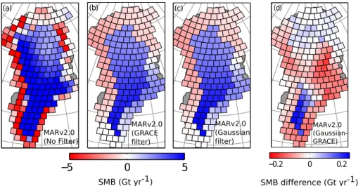
and temporally filtered to match GRACE-LM. The e_ffect of spatial smoothing on the MAR v2.0 aggregated outputs (Fig. 2a), along with the impact of di_fferent constraint

10

regions above and below 2000 m in elevation, can be seen in Fig. 2b, which shows the mean 2000–2010 MAR v2.0 outputs filtered using the resolution matrix. As expected, the spatial filtering decreases the magnitude of mass change for individual mascons by redistributing mass change accross other surrounding mascons.

Unfortunately, the methods discussed above (hereafter referred to as “GRACE-LM

15

filtering”) are computationally expensive and time consuming to perform. We only ap-plied GRACE-LM filtering to MAR v2.0 outputs as only these outputs were available when the GRACE-LM filtering procedure was applied. To filter MAR v3.5.2 and ISSM data, we employed an approximation to the GRACE-LM filtering procedure, which is described further below.

20

2.4.3 A Gaussian approximation to GRACE-LM filtering

As discussed by Luthcke et al. (2013), the leakage associated with individual GRACE-LM mascons is roughly equivalent to a spatial Gaussian filter with a radius of 300 km, with the mascons within a 600 km radius accounting for almost 100 % of the mass changes within a mascon. To allow for spatial filtering of MAR v3.5.2 and ISSM outputs,

25

(13)

TCD

9, 6345–6393, 2015

and GRACE

Title Page

Tables Figures

◭ ◮

Back Close

Full Screen / Esc

Discussion

P

a

per

|

Discussion

P

a

per

|

Discussion

P

a

per

|

Discussion

P

a

per

|

distribution (x₋µ) and a standard deviation (σ) as:

g(x)₌ 1 σ√2π

e−12(

x−µ σ )

2

(5)

We used a gaussian function to weight the data for all surrounding mascons (j) as a function of radial distance from a central mascon (i). In this case,x₋µis replaced by the distance from a central location to another mascon (r_{i j}), and a discrete

approxi-5

mation to the Gaussian is used, as follows:

g(r_{i j})=e−

1 2

_rij

σi

2

(6)

w_j ₌_P_ng(ri j) j=1g(ri j)

(7)

The weight, w_j, assigned to a given mascon, j, at a distance r_{i j} from mascon i, is given by the value of the Gaussian function at the center of masconj divided by the

10

sum of all Gaussian values surrounding masconi. A different σ_i value is chosen for each mascon.

We further modify Eq. (7) to account for the constraint regions discussed in the pre-vious section, which for the GrIS, includes areas above and below 2000 m in eleva-tion (Luthcke et al., 2013). For a given mascon within a constraint region (masconi),

15

weights for mascons outside of the constraint region were multiplied by a leakage pa-rameter,λ_j, which was set to 1 within the constraint region, and a fixed value between 0 and 1 outside of the constraint region. Accounting for these constraints, Eq. (7) be-comes:

w_j ₌_P_ng(ri j)λi j j=1g(ri j)λi j

(8)

20

(14)

TCD

9, 6345–6393, 2015

and GRACE

Title Page

Tables Figures

◭ ◮

Back Close

Full Screen / Esc

Discussion

P

a

per

|

Discussion

P

a

per

|

Discussion

P

a

per

|

Discussion

P

a

per

|

The weights for mascons j surrounding a central mascon i are then used to cre-ate a weighted average of mass change for mascon i (_∆m_i_,new) as a function of the modeled changes for masconi (∆m_i) and masconsj (∆m_j):

∆m_i_,new_{= ∆}m_iw_i₊ n X

j=1

∆m_jw_j (9)

Finally, we added a time component to the filtering procedure, as the regularization

5

matrix (Phh) discussed in Sect. 2.4.2 also includes a temporal component (Sabaka et al., 2010), and because GRACE-LM-filtering alters both the amplitude and timing of the seasonal cycle of mass change (as discussed in Sect. 2.4.5). After applying the spatial filter described by Eqs. (6) and (8), timeseries of cumulative mass from MAR v2.0 were interpolated onto GRACE-LM time-intervals. We then applied a temporal

10

Gaussian filter to the cumulative mass timeseries for each mascon, using the temporal radius_∆t_t₀_tk, wheret_k is a time before or after the timet₀and_∆t_t₀_tk₌_|t_k₋t₀_|:

g(_∆t_t₀_tk)₌e−

1 2

_∆tt

0tk σ_time

(10)

w_tk=_P_mg(∆tt0tk)

k=ng(∆tt0tk)

(11)

wherenis the first value in the timeseries being filtered andmis the last value.

15

We applied the spatial and temporal filters discussed above to the aggregated un-filtered MAR v2.0 data, and compared the resulting cumulative mass timeseries’ from each mascon to the GRACE-LM filtered MAR v2.0 timeseries. Two filtering procedures were employed, one in which only spatial filtering was performed, and another in which both spatial and temporal filtering were performed to determine the impact of

tem-20

(15)

TCD

9, 6345–6393, 2015

and GRACE

Title Page

Tables Figures

◭ ◮

Back Close

Full Screen / Esc

Discussion

P

a

per

|

Discussion

P

a

per

|

Discussion

P

a

per

|

Discussion

P

a

per

|

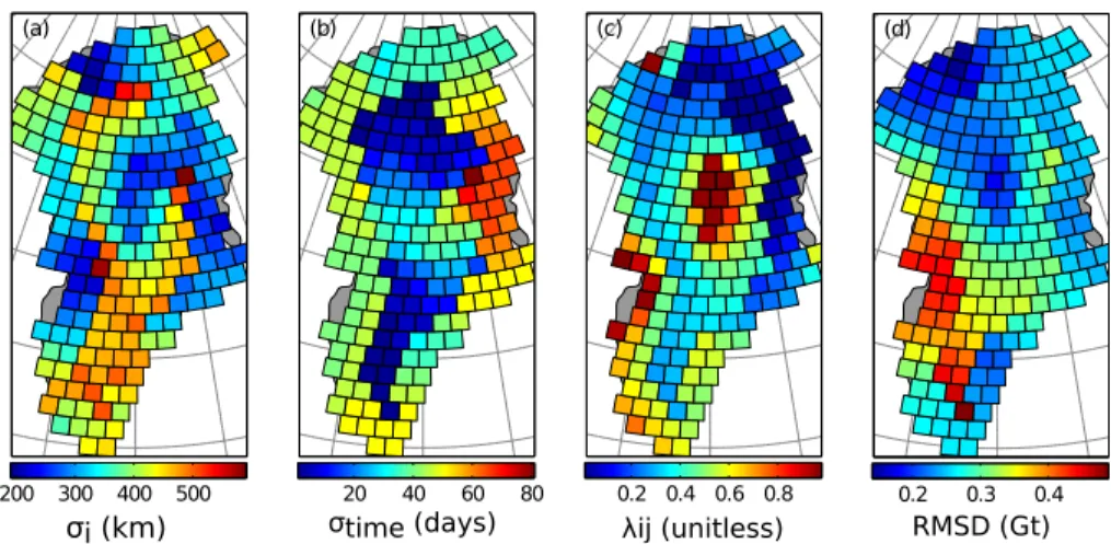
Initially, the same values ofσ_I,σ_time, and λ_{i j} were used for all mascons i, but it was found that by spatially varying the values of these parameters the errors were reduced. We also set λ_{i j} equal to zero outside of the island of Greenland as defined by the GRACE-LM mascons, as this improved the agreement with the GRACE-LM-filtered re-sults. Values ofσ_i were varied at 10 km increments over a range of 1 to 600 km, while

5

values ofσ_time ranged between 1 and 91 days at increments of 5 days, andλ_{i j} ranged between 0 and 1 at increments of 0.01. We tried larger values ofσ_i beyond the indi-cated range at larger increments, but did not find a reduction in RMSE for values larger than 600 km.

Average Gaussian-filtered MAR v2.0 SMB (with both spatial and temporal filtering

10

applied) for the period 2003–2010 is shown in Fig. 2c. The Gaussian-filtered MAR v2.0 SMB is similar to GRACE-LM-filtered SMB. Differences between the GRACE-LM-filtered and Gaussian-GRACE-LM-filtered results (Fig. 2d) are an order of magnitude smaller than the average SMB values (ranging from₋0.2 to 0.2 vs.₋2 to 5 Gt), although in some regions where trends in SMB are small, the di_fferences are a large percentage of the

15

average SMB. Optimal values forσ_i,σ_time, andλ_{i j} and the RMSE for the Gaussian vs. the GRACE-LM-filtered MAR v2.0 data are shown in Fig. 3. Further discussion of the impacts of filtering on model outputs is provided in Sect. 2.4.5.

2.4.4 Application of Gaussian filters and seasonal cycle analysis

Following the choice of the optimal Gaussian filter using MAR v2.0, we applied the

20

same chosen filter to MAR v3.5.2 and ISSM data forced by MAR v3.5.2, aggregated to the GRACE-LM grid. MAR v3.5.2 exhibits a less negative SMB along the Greenland coast and GrIS margins and a less positive SMB within the GrIS interior (Fig. S1 in the Supplement) compared with MAR v2.0 (as there is more coastal accumulation and less interior accumulation in MAR v3.5.2). These di_fferences do not a_ffect our ability

25

(16)

TCD

9, 6345–6393, 2015

and GRACE

Title Page

Tables Figures

◭ ◮

Back Close

Full Screen / Esc

Discussion

P

a

per

|

Discussion

P

a

per

|

Discussion

P

a

per

|

Discussion

P

a

per

|

then interpolated onto GRACE-LM time steps, and temporal filtering was performed. We then summed the timeseries of cumulative mass change from MAR v3.5.2 and ISSM, to generate timeseries of integrated MB.

We examined differences between the modeled and GRACE-LM seasonal cycles of cumulative mass change by first interpolating filtered cumulative model and

GRACE-5

LM timeseries to a daily temporal resolution, removing linear trends from the time-series, and averaging the data for a given day of the year across all available years. This was performed for the GrIS-wide timeseries, as well as for individual mascons and GrIS sub-regions. A two-year composite seasonal cycle was constructed for GRACE-LM and model data, and the timing of the highest local maximum and lowest local

10

minimum in this cycle were identified.

GRACE data from Luthcke et al. (2013) include estimates of the error associated with the timeseries of cumulative mass change for each mascon. When examining ag-gregated data, we summed the error for all mascons. The error for a given day for the GRACE-LM seasonal cycle was determined to be the total GRACE-LM error for the

cu-15

mulative timeseries divided by√n, wherenwas the number of years being averaged. Errors in the GRACE-LM timeseries can lead to errors in the timing of the seasonal cycle because random errors can cause a shift in the timing of a local maximum or minimum point. To account for these errors, we performed 10 000 Monte Carlo simu-lations with the GRACE-LM seasonal data, assuming that the errors in the timeseries

20

were normally distributed. For each of these simulations, we identified the local maxi-mum and minimaxi-mum peaks in the seasonal cycle, allowing us to generate a distribution of dates for maximum and minimum peaks. If the model peaks fell outside of the 95 % confidence interval for this distribution, the timing of the GRACE-LM and model peaks was deemed to differ.

25

2.4.5 Effect of filtering on seasonal variations in mass

(17)

TCD

9, 6345–6393, 2015

and GRACE

Title Page

Tables Figures

◭ ◮

Back Close

Full Screen / Esc

Discussion

P

a

per

|

Discussion

P

a

per

|

Discussion

P

a

per

|

Discussion

P

a

per

|

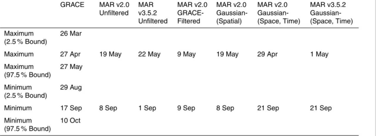
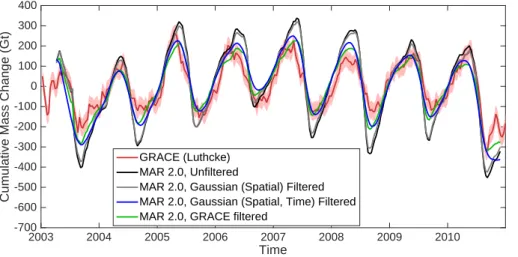
cumulative timeseries of GrIS-wide mass changes, in relation to the seasonal cycle of mass change from GRACE-LM. While it is not possible to compare GRACE-derived mass changes directly to MAR, given that GRACE also records the effects of changes in DMB, a comparison of de-trended timeseries of cumulative mass can be performed, if it is assumed that seasonal variations in ice discharge are small relative to those

5

of SMB. A qualitative comparison of de-trended unfiltered and filtered MAR v2.0 and GRACE-LM cumulative mass timeseries for the GrIS over 2003–2010 (Fig. 4), sug-gests that this is a reasonable first-order assumption for the entire GrIS. Fluctuations in mass, coinciding with net loss of mass during summer months, and net gain of mass during winter months, are captured by both GRACE-LM and MAR v2.0. The average

10

seasonal cycle of cumulative mass change in Fig. 5a indicates a larger amplitude of mass fluctuations for unfiltered and spatially Gaussian-filtered MAR v2.0 results (of 524 and 500 Gt respectively) relative to GRACE-LM (287_±30 Gt), and a closer agreement between the amplitudes of LM-filtered MAR v2.0 data (339 Gt) and GRACE-LM. On average, during periods of net ablation, GRACE-LM begins losing mass earlier

15

(by 25 days), and starts gaining mass later (by 8 days) as compared with MAR v2.0 unfiltered data (Table 1). GRACE-LM-filtering changes the timing of the start of mass loss such that the period of simulated mass loss begins 10 days sooner, extending the length of the mass loss period.

When both spatial and temporal Gaussian filtering are applied to the MAR v2.0 data,

20

the amplitude of the seasonal cycle is reduced (to 351 Gt), resulting in a better agree-ment with GRACE-LM and with the GRACE-LM-filtered MAR v2.0 data (Fig. 5a). The timing of peaks in maximum and minimum mass are also changed, with the temporally Gaussian-filtered MAR v2.0 data exhibiting an extended period of mass loss (145 days) relative to that of the GRACE-LM-filtered MAR v2.0 data (123 days), resulting in the

fil-25

(18)

TCD

9, 6345–6393, 2015

and GRACE

Title Page

Tables Figures

◭ ◮

Back Close

Full Screen / Esc

Discussion

P

a

per

|

Discussion

P

a

per

|

Discussion

P

a

per

|

Discussion

P

a

per

|

Temporal Gaussian-filtering improves the agreement between the Gaussian-filtered MAR v2.0 timeseries and the GRACE-LM-filtered timeseries in terms of amplitude, and lengthens the period of net ablation (perhaps too much relative to the period for GRACE-LM-filtered data). For both methods of Gaussian filtering, the timing of the peaks for filtered MAR v2.0 data fall within the 95 % confidence bounds on the timing

5

of the GRACE-LM seasonal cycle.

The comparison of GRACE and MAR timeseries and seasonal cycles in the case of MAR v3.5.2 (Figs. S2 and 5b respectively) is similar to that for MAR v2.0. MAR v3.5.2 features a seasonal cycle of smaller amplitude, likely as a result of snow falling more frequently along the coast, where it is more likely to be balanced by ablation

10

during periods of net accumulation, and where it mitigates ablation during periods of net mass loss. The Gaussian filtering has a similar effect on the MAR v3.5.2 outputs, which are similar in timing to MAR v2.0 outputs (Table 1), by reducing the amplitude of seasonal variability and extending the length of the ablation season to be similar to that of GRACE-LM (Fig. 5b and Table 1). In our analysis of ISSM and MAR v3.5.2

15

outputs, we have chosen to focus on results obtained with temporal Gaussian filtering applied, as it results in reduced errors relative to the GRACE-LM filtering method. We consider this to be a statistically conservative approach. Because we are not able to fully capture the effect of filtering on the timing of the seasonal cycle, we choose the filter that brings the timing of the seasonal cycle closer to that of GRACE-LM. Thus, in

20

locations where the timing of the Gaussian-filtered cycle falls outside of the range of dates from GRACE-LM, it is very likely that there is a difference between the modeled and GRACE-LM seasonal cycles that is not associated with filtering. In locations where the timing of the Gaussian-filtered cycle falls within the range of dates from GRACE-LM, we cannot confirm a difference.

(19)

TCD

9, 6345–6393, 2015

and GRACE

Title Page

Tables Figures

◭ ◮

Back Close

Full Screen / Esc

Discussion

P

a

per

|

Discussion

P

a

per

|

Discussion

P

a

per

|

Discussion

P

a

per

|

3 Results

3.1 Trends and spatial differences in modelled vs. measured mean MB

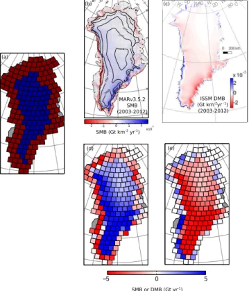
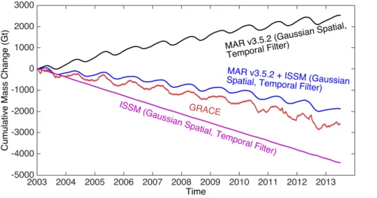
We first examine the timeseries of GrIS cumulative mass as simulated by MAR v3.5.2, ISSM, and GRACE-LM over the 2003–2012 period, as shown in Fig. 6. MAR v3.5.2 cumulative SMB shows a net accumulation of mass over Greenland (of 247 Gt yr−1),

5

which varies seasonally in response to cycles of melting and accumulation. ISSM ex-hibits a net loss of mass (₋426 Gt yr−1on average), with little seasonal variability rela-tive to the long-term trend. There is a small seasonal cycle in ISSM dynamics driven by the SMB cycle (visible in the detrended timeseries shown in Fig. S3) which com-plements the mass changes from MAR (increased mass loss from MAR leads to

de-10

creased mass loss from ISSM, and vice versa), with an amplitude roughly an order of magnitude smaller than the SMB fluctuations. Together, ISSM and MAR v3.5.2 results produce a net loss of mass over 2003–2012, although the trend in simulated mass loss (₋179 Gt yr−1) is smaller in magnitude than that of GRACE-LM (₋240 Gt yr−1) by 61 Gt yr−1.

15

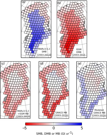
The roughly complementary nature of modeled SMB and DMB is evident on a sub ice-sheet wide scale, as indicated by the unfiltered MAR v3.5.2 and ISSM 2000–2012 mean SMB and DMB (Fig. 1) as well as the Gaussian filtered data (Fig. 7a and b). Areas with a large positive SMB from MAR v3.5.2 show large dynamic mass loss from ISSM (e.g. areas higher than 2000 m in elevation), while areas with negative SMB

20

from MAR v3.5.2 show smaller losses from ISSM. Summing SMB and DMB from MAR v3.5.2 and ISSM produces the pattern of MB shown in Fig. 7c, which indicates that the majority of modeled mass loss for the 2003–2012 period occurs below 2000 m in elevation. This is similar to pattern of MB from GRACE-LM (Fig. 7d). A map of the di_fference between modeled and GRACE-LM MB (Fig. 7e) indicates that the majority

25

(20)

TCD

9, 6345–6393, 2015

and GRACE

Title Page

Tables Figures

◭ ◮

Back Close

Full Screen / Esc

Discussion

P

a

per

|

Discussion

P

a

per

|

Discussion

P

a

per

|

Discussion

P

a

per

|

2000 m, overall mass loss is underestimated by 92 Gt yr−1(with a trend of₋150 Gt yr−1 as compared with₋242 Gt yr−1 from GRACE). For areas above 2000 m, GRACE-LM suggests a mass gain of₊3 Gt yr−1while the models suggest a loss of₋30 Gt yr−1.

The di_fferences between simulated and GRACE-LM MB may be due to a modeled MAR v3.5.2 SMB that is too high below 2000 m in elevation, or alternately, to

simu-5

lated velocities that are underestimated in ISSM and vice versa at higher elevations. A comparison of ice thicknesses from Morlighem et al. (2015) and velocities from Rig-not and MougiRig-not (2012) with ISSM velocities and thicknesses for 1 January 2003 is shown in Fig. S4. Some di_fferences may result from the model outputs and observa-tions not being coincident in time, but Fig. S3 indicates that temporal variability in ISSM

10

is small (<10 %) relative to long-term changes. (This relatively small variability is to be expected given that the ISSM simulation used here only considers forcing from SMB and not other factors that may lead to larger fluctuations in ice motion.) In particular, the ice thickness is underestimated in central northwestern Greenland, but overesti-mated along the coast and in southern Greenland. In areas of underestioveresti-mated

thick-15

ness, ISSM velocities tend to be underestimated, resulting in a dynamic accumulation of mass that should be leaving the ice sheet. It is difficult to determine if the observed differences are a result of errors in the MAR v3.5.2 SMB forcing (as the spinup relies primarily on the simulated SMB for forcing), simplifications to full-Stokes ice flow in ISSM, processes not considered in the ISSM simulation such as the role of hydrology

20

in ice dynamics and ice–ocean interactions, or errors associated with the assumption that during the spin-up period, the ice sheet is in steady state. The assumption of 2-D flow (SSA) in the current ISSM simulation probably contributes to errors in dynamic mass balance, particularly at higher elevations, but it is not clear whether this would lead to faster or slower ice flow. A comparison between MAR v3.5.2 SMB and in situ

25

(21)

be-TCD

9, 6345–6393, 2015

and GRACE

Title Page

Tables Figures

◭ ◮

Back Close

Full Screen / Esc

Discussion

P

a

per

|

Discussion

P

a

per

|

Discussion

P

a

per

|

Discussion

P

a

per

|

tween model results and GRACE-LM is the 25 km resolution of the MAR outputs used in this study. ISSM is forced by a downscaled version of MAR v3.5.2. Using a higher resolution simulation or downscaled outputs could result in different SMB estimates (e.g. Franco et al., 2012). This could be particularly important along the borders of the GrIS, or for mountainous areas outside the ice sheet boundaries. In these areas,

5

high spatial variability of topography can strongly influence SMB. To properly identify the source of the differences, further independent evaluations of MAR SMB and ISSM DMB are needed.

3.2 Seasonal mass changes from MAR, ISSM and GRACE

The average seasonal cycle of filtered cumulative MAR v3.5.2+ISSM for the 2003

10

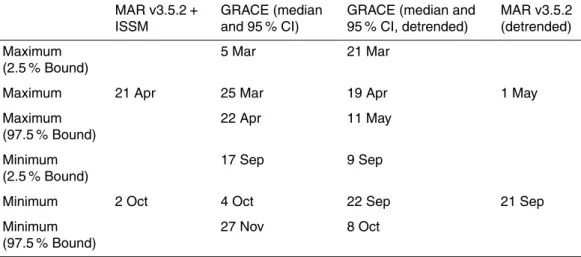
through 2012 period agrees well with that of GRACE-LM, as shown in Fig. 8a and Table 2. The amount of mass loss during the period of net ablation is similar for MAR v3.5.2+ISSM (333 Gt) and GRACE-LM (355_±32 Gt). The dates of simulated maximum and minimum mass fall within the range of uncertainty for these dates from GRACE-LM. It is possible, however, that di_fferences in modeled and GRACE-LM trends alter the

15

timing of the seasonal cycle, because changing the overall trend of a timeseries can al-ter the timing of local maxima and minima by alal-tering local rates of change. Therefore, we also show the seasonal cycle for the de-trended timeseries in Fig. 8b and Table 2. For the de-trended seasonal cycle, the timing of the seasonal maximum occurs roughly 1 month before the maximum peak from the original seasonal cycle, and the timing of

20

the seasonal minimum occurs roughly 1 week earlier for both MAR v3.5.2₊ISSM and GRACE-LM. In either case, the model timing for the filtered model data falls within the range of dates from GRACE-LM, and therefore we cannot confirm any difference be-tween the modeled and GRACE-LM Greenland-wide seasonal cycles of mass change. The results are consistent with the comparison between the detrended MAR v3.5.2

25

(22)

TCD

9, 6345–6393, 2015

and GRACE

Title Page

Tables Figures

◭ ◮

Back Close

Full Screen / Esc

Discussion

P

a

per

|

Discussion

P

a

per

|

Discussion

P

a

per

|

Discussion

P

a

per

|

increasing discharge during periods of high SMB, and vice versa, with an amplitude roughly an order of magnitude smaller than that of MAR (Fig. S5). As noted earlier, this magnitude of simulated flow variability is the expected response to the SMB forcing applied to ISSM.

3.3 Spatial variability in the seasonal cycle from MAR, ISSM and GRACE 5

Maps of the timing of peaks in the seasonal cycle of de-trended cumulative mass change from GRACE-LM (Fig. 9) suggest that the timing of seasonal cycle peaks is spatially variable. Maps of the median GRACE-LM date for the maximum and minimum peaks (Fig. 9a and d) show that in some locations (e.g. northwest Greenland), GRACE-LM suggests that the peak in the seasonal cycle can occur as early as 1 November

10

(i.e. mass loss begins during the fall), where in other areas it occurs as late as 1 July (for an area in north Greenland). The range of possible dates suggested by 95 % of the GRACE-LM distribution, when taking into account GRACE-LM uncertainty, is fairly large, spanning the full 1 November to 1 July period in some locations in northern Greenland (Fig. 9b, c, e and f), but spatial di_fferences in seasonal timing are preserved

15

even with these large ranges. The GRACE-LM data suggest that the period of net mass loss begins in late winter and ends in early summer in the northwestern portion of the ice sheet, while in most other parts of the ice sheet, mass loss begins in early or late spring, and mass begins to increase again beginning in late autumn. The pe-riod of summer mass loss over most of the ice sheet is consistent with what would

20

be expected, given the cycle of climate forcing (warm conditions leading to increased melt), but the timing of the cycle in the northwest suggests that other processes may dominate seasonal variability in that region.

MAR v3.5.2₊ISSM suggest a more uniform pattern of timing in seasonal cycle peaks (Fig. 10a and b), consistent with the SMB forcing. The models suggest that

25

(23)

TCD

9, 6345–6393, 2015

and GRACE

Title Page

Tables Figures

◭ ◮

Back Close

Full Screen / Esc

Discussion

P

a

per

|

Discussion

P

a

per

|

Discussion

P

a

per

|

Discussion

P

a

per

|

ending_∼1 month later for mascons below 2000 m in elevation relative to those above 2000 m in elevation. These results are consistent with what would be expected given warmer temperatures at lower elevations and a longer period available for melting.

For many mascons in the Northwest, the modeled cycle maximum and minimum peaks can occur up to 3 months after and 2 months before the GRACE-LM peaks

5

(Fig. 10c and d), with differences of _∼1 month being quite common. Given the rela-tively large uncertainty in the timing of the GRACE-LM peaks, the model peaks often fall within the distribution of peaks from GRACE-LM. Along the northwest coast, however, the timing of the seasonal maximum occurs in May according to the models, roughly one or two months after the 95 % confidence limit on the timing of maximum mass from

10

GRACE-LM, and more than three months after the median peak from GRACE-LM. Despite the large uncertainty in the GRACE timing, the timing of GRACE-LM peaks tends to be clustered in groups, suggesting that the spatial variations in GRACE-LM timing are not random, but actually reflect seasonal variations in mass not captured by the models. The timing of seasonal minimum falls within 95 % of the distribution from

15

GRACE-LM, with the exception of six mascons at high elevations along the southeast coast.

3.4 The average seasonal cycle within ice sheet sub-regions

In order to further examine discrepancies at regional scales, we created eight sub-regions of the GrIS based on the median timing of the maximum and minimum peaks

20

of the average de-trended annual cycle from GRACE-LM (Fig. 9a and d). Mascons were grouped together if the timing of their maximum and minimum peaks were within 30 days of each other. The eight sub-regions are shown in Fig. 11a, along with the average seasonal cycle from four of these sub-regions (Fig. 11b–e). The average cycles for other regions are provided in Fig. S6a–d in the Supplement. The average

25

(24)

TCD

9, 6345–6393, 2015

and GRACE

Title Page

Tables Figures

◭ ◮

Back Close

Full Screen / Esc

Discussion

P

a

per

|

Discussion

P

a

per

|

Discussion

P

a

per

|

Discussion

P

a

per

|

a result of the SMB signal. For Region 6 (Fig. 11e), the maximum modeled mass oc-curs in early May (although the ice sheet does not appear to start losing a substantial amount of mass until July), while the GRACE-LM peak occurs in early November. The entire modeled cycle appears to be offset by three months relative to GRACE-LM in this region, although seasonal mass changes are relatively small (on the order of 5 Gt).

5

For Regions 4 and 5 (Fig. 11c and d), the model maximum and minimum peaks fall within the distribution for GRACE-LM peaks. For Regions 2, 7 and 8 (Fig. S6a, c, and d in the Supplement) the cycles are similar to those of Regions 1 and 6. For Region 3 (Fig. S6b in the Supplement), the cycle is similar to the cycle of Region 4, except for a sharp peak in mass in early July, which leads the GRACE-LM peak to occur after the

10

peak from the models.

Dividing the GrIS into high and low elevation areas (above and below 2000 m in elevation) also produces differences in the seasonal cycle (Fig. 12). For areas below 2000 m in elevation (Fig. 12a), there is a good agreement between the GRACE-LM and simulated seasonal cycles; the timing of MAR v3.5₊ISSM maximum and minimum

15

peaks fall within the distribution of peaks for GRACE-LM as the signal is dominated by the summer surface mass loss. For areas higher than 2000 m in elevation (Fig. 12b), the period of simulated net mass loss is shortened relative to that of GRACE-LM. The good agreement between cycles at low elevations suggests that the timing of ablation and accumulation at low elevations on an ice sheet wide scale is well captured by MAR

20

v3.5.2₊ISSM.

As for Greenland-wide fluctuations in mass, most of the simulated seasonal variabil-ity within sub-regions of the ice sheet is dominated by MAR, as expected given that the only forcing applied to ISSM is the SMB from MAR. ISSM exhibits a seasonal cycle that is a lagged inverse of the MAR cycle with less than 10 % of the amplitude of MAR v3.5.2

25

(25)

TCD

9, 6345–6393, 2015

and GRACE

Title Page

Tables Figures

◭ ◮

Back Close

Full Screen / Esc

Discussion

P

a

per

|

Discussion

P

a

per

|

Discussion

P

a

per

|

Discussion

P

a

per

|

The differences in the GRACE-LM and modeled seasonal cycles within individual regions and at high elevations seem unlikely to be caused by errors in the simulated timing of surface ablation, as they occur either during times of the year when melting does not occur at the surface (i.e. the “early” start to the period of net mass loss in the northeast from November through February), or in areas where the net ablation due

5

to melting is small (i.e. above 2000 m in elevation). The results therefore suggest that the observed changes could be associated with errors in seasonal accumulation from MAR v3.5.2, or processes not currently incorporated into ISSM, which induce seasonal fluctuations in ice discharge or liquid water. These processes are difficult to validate, and therefore it is difficult to determine which processes are most responsible for the

10

observed di_fferences. As discussed in the following section, significant seasonal vari-ations in glacier velocities have been observed and could contribute to the observed discrepancies. Additionally, although the GRACE-LM solution includes error estimates associated with the forward models used in GRACE processing, there is also a possi-bility that other non-ice-sheet-related processes may contribute to the di_fferences.

15

4 Discussion and conclusions

The above results show several areas of agreement as well as areas of disagreement between modeled and GRACE-derived Greenland mass balance. We have shown that in order to compare spatial and temporal variations in GrIS mass from RCM, ISM re-sults and the GRACE-LM solution, it is necessary to spatially and temporally filter the

20

model outputs. We have developed a Gaussian approximation to the GRACE-LM res-olution operator, which accurately captures the effect of the GRACE-LM solution on spatial variations in mean MB. We also find that applying temporal filtering reduces di_fferences between the modeled and GRACE-LM seasonal cycles. We have there-fore implemented a temporal Gaussian filter with the goal of reproducing this effect.

25

(26)

TCD

9, 6345–6393, 2015

and GRACE

Title Page

Tables Figures

◭ ◮

Back Close

Full Screen / Esc

Discussion

P

a

per

|

Discussion

P

a

per

|

Discussion

P

a

per

|

Discussion

P

a

per

|

the period of mass loss simulated by the models further than the period obtained from GRACE-LM filtering. As the filter brings the timing of the Greenland-wide cycle of mass changes closer to that of GRACE-LM, in cases where it disagrees with the Greenland-wide cycle, differences in the timing of the modeled and GRACE-LM cycle are likely.

A comparison between Gaussian-filtered MAR v3.5.2₊ISSM and GRACE-LM

5

Greenland mass trends for 2003–2012 indicates that the models tend to underesti-mate the magnitude of this mass loss, as a result of underestiunderesti-mated mass loss below 2000 m in elevation. This di_fference is either due to an overestimation of SMB from MAR v3.5.2 in low elevation areas, or to intrinsic errors in ice flow from ISSM. MAR v3.5.2 SMB for low elevation areas is higher than that of MAR v2.0, in part due to a

rel-10

atively high bare ice albedo (as described by Alexander et al., 2014; a higher albedo persists despite modifications made to MAR v3.5.2 albedo), and in part due to a shift in precipitation from high to low elevation areas. A comparison at in situ stations suggests that MAR v3.5.2 SMB is closer to in situ measurements (Colgan et al., 2015), but few SMB measurements are available within the GrIS ablation area. The only means of

15

determining the relative contribution of ISSM and MAR v3.5.2 to underestimated mass loss would be to conduct an independent evaluation of each model against DMB and SMB estimates over large portions of the GrIS; this analysis is beyond the scope of this study.

We examined the mean seasonal cycles of de-trended cumulative mass change from

20

GRACE-LM and MAR v3.5.2₊ISSM as a means of examining the ability of the models to capture mass changes at a relatively high spatial and temporal resolution. We have shown that on a Greenland-wide scale, the timing of modeled and GRACE seasonal cycles agree, within the limits of GRACE uncertainty, but on sub-ice-sheet-wide scales, there are significant differences in the timing of annual cycle peaks. On the scale of

in-25

(27)

TCD

9, 6345–6393, 2015

and GRACE

Title Page

Tables Figures

◭ ◮

Back Close

Full Screen / Esc

Discussion

P

a

per

|

Discussion

P

a

per

|

Discussion

P

a

per

|

Discussion

P

a

per

|

reflect real differences in the seasonal variability within different regions, particularly as the di_fferences are not random, but spatially clustered. In particular, in northwestern Greenland, the simulated period of mass loss is shorter than that of GRACE-LM, and the timing of the simulated maximum in the seasonal cycle occurs up to three months after the GRACE-LM peak in some areas.

5

Spatial and seasonal differences in the seasonal cycle may result from various fac-tors including (1) underestimation or overestimation of accumulation and ablation by MAR v3.5.2, (2) cycles of ice sheet motion associated with processes not incorporated into ISSM, (3) cycles of water storage and release, and (4) errors in the GRACE-LM solution. We have attempted to account for the last factor by considering the impact

10

of errors of the GRACE-LM solution estimated by Luthcke et al. (2013) on the timing of the seasonal cycle, and by filtering our model results to match GRACE-LM. How-ever, as GRACE does not provide direct observations of mass changes, and different methods of processing can produce somewhat di_fferent mass change solutions (Shep-herd et al., 2012), it is possible that some of the observed discrepancies may be due

15

to errors not considered in this solution. With regard to MAR v3.5.2 accumulation, the Colgan et al. (2015) study suggests that MAR v3.5.2 e_ffectively captures spatial varia-tions in SMB, but few observavaria-tions of SMB are available in areas of net ablation. The seasonal cycle of MAR v3.5.2 has not been evaluated against observations, as few sub-annual estimates of accumulation are available. With regard to GrIS discharge, an

20

analysis of ISSM annual discharge has not been conducted, although comparison with satellite-derived ice velocities suggests that ISSM velocities may be underestimated in some areas at the ice sheet margins. Data on seasonal velocities are not available for the entire GrIS, but various studies have indicated seasonal variations in the flow of GrIS glaciers occur, particularly in association with meltwater that reaches the ice

25