www.atmos-chem-phys.net/15/7703/2015/ doi:10.5194/acp-15-7703-2015
© Author(s) 2015. CC Attribution 3.0 License.
Climate-forced air-quality modeling at the urban scale: sensitivity to
model resolution, emissions and meteorology
K. Markakis1, M. Valari1, O. Perrussel2, O. Sanchez2, and C. Honore2
1Laboratoire de Meteorologie Dynamique, IPSL Laboratoire CEA/CNRS/UVSQ, Ecole Polytechnique, 91128 Palaiseau CEDEX, France
2AIRPARIF, Association de surveillance de qualité de l’air en Île-de-France, 7 rue Crillon, 75004, Paris, France
Correspondence to: K. Markakis ([email protected])
Received: 12 November 2014 – Published in Atmos. Chem. Phys. Discuss.: 20 February 2015 Revised: 12 June 2015 – Accepted: 1 July 2015 – Published: 14 July 2015
Abstract. While previous research helped to identify and pri-oritize the sources of error in air-quality modeling due to an-thropogenic emissions and spatial scale effects, our knowl-edge is limited on how these uncertainties affect climate-forced air-quality assessments. Using as reference a 10-year model simulation over the greater Paris (France) area at 4 km resolution and anthropogenic emissions from a 1 km reso-lution bottom-up inventory, through several tests we estimate the sensitivity of modeled ozone and PM2.5concentrations to different potentially influential factors with a particular inter-est over the urban areas. These factors include the model hor-izontal and vertical resolution, the meteorological input from a climate model and its resolution, the use of a top-down emission inventory, the resolution of the emissions input and the post-processing coefficients used to derive the temporal, vertical and chemical split of emissions. We show that urban ozone displays moderate sensitivity to the resolution of emis-sions (∼8 %), the post-processing method (6.5 %) and the horizontal resolution of the air-quality model (∼5 %), while annual PM2.5levels are particularly sensitive to changes in their primary emissions (∼32 %) and the resolution of the emission inventory (∼24 %). The air-quality model horizon-tal and vertical resolution have little effect on model predic-tions for the specific study domain. In the case of modeled ozone concentrations, the implementation of refined input data results in a consistent decrease (from 2.5 up to 8.3 %), mainly due to inhibition of the titration rate by nitrogen ox-ides. Such consistency is not observed for PM2.5. In contrast this consistency is not observed for PM2.5. In addition we use the results of these sensitivities to explain and quantify the discrepancy between a coarse (∼50 km) and a fine (4 km)
resolution simulation over the urban area. We show that the ozone bias of the coarse run (+9 ppb) is reduced by∼40 % by adopting a higher resolution emission inventory, by 25 % by using a post-processing technique based on the local in-ventory (same improvement is obtained by increasing model horizontal resolution) and by 10 % by adopting the annual emission totals of the local inventory. The bias of PM2.5 con-centrations follows a more complex pattern, with the positive values associated with the coarse run (+3.6 µg m−3), increas-ing or decreasincreas-ing dependincreas-ing on the type of the refinement. We conclude that in the case of fine particles, the coarse sim-ulation cannot selectively incorporate local-scale features in order to reduce its error.
1 Introduction
Recent epidemiological findings stress the need to resolve the variability of pollutant concentrations at the urban scale. The International Agency for Research on Cancer recently classified outdoor air pollution as a “leading environmental cause of cancer deaths” (Loomis et al., 2013) while new find-ings reveal that living near busy roads substantially increases the total burden of disease attributable to air pollution (Pas-cal et al., 2013). Research on future projections of air-quality should be addressed primarily at such scale especially given the fact that the efforts to mitigate air-pollution are more in-tense in areas where the largest health benefits are observed (Riahi et al., 2011).
atmo-spheric feedback. A significant portion of the published lit-erature on this issue uses global-scale models to focus on the impact of climate on tropospheric ozone at the global or re-gional scale (Brasseur et al., 1998; Liao et al., 2006; Prather et al., 2003; Szopa et al., 2006; Szopa and Hauglustaine, 2007). More recent studies have integrated advanced chem-istry schemes capable of resolving the variability of pollu-tant concentrations at regional scale, which spans from sev-eral hours up to a few days, with chemistry transport mod-els (CTMs) (Colette et al., 2012, 2013; Forkel and Knoche, 2006, 2007; Hogrefe et al., 2004; Katragkou et al., 2011; Kelly et al., 2012; Knowlton et al., 2004; Lam et al., 2011; Langner et al., 2005, 2012; Nolte et al., 2008; Szopa and Hauglustaine, 2007; Tagaris et al., 2009; Zanis et al., 2011). Global models with a typical resolution of a few hundreds of kilometers and regional CTMs used at resolutions of a few tens of kilometers, and their parameterization of physical and chemical processes make them inadequate for modeling air-quality at the urban scale (Cohan et al., 2006; Forkel and Knoche, 2007; Markakis et al., 2014; Sillman et al., 1990; Tie et al., 2010; Valari and Menut, 2008; Valin et al., 2011; Vautard et al., 2007).
The challenge we face is how to model climate-forced at-mospheric composition with CTMs at fine resolution over urban areas, where emission gradients are particularly sharp, without introducing large errors due to emissions and mete-orology related uncertainties as well as to CTMs numerical resolution. In the absence of plume-in-grid parameterization, emissions in CTMs are instantly mixed within the volume of model grid-cells before chemical reaction transport and mixing take place. When the volume of these cells is large compared to the characteristic time scale of these processes, sub-grid scale errors occur such as over-dilution of emissions leading to unrealistic representation of urban-scale chem-istry such as ozone titration. The resolution of meteorologi-cal modeling is another issue: Leroyer et al. (2014) argue that only high-resolution meteorological modeling can correctly capture the urban heat island, also Flagg and Taylor (2011) showed that high-resolution modeling is very much depen-dent on the resolution of the surface layer input data.
Another key issue is the representativeness of top-down emission inventories over cities. The starting point of these inventories is annual totals for families of pollutants at conti-nental, regional or national scale that are temporally and spa-tially downscaled based on proxies such as land-use and pop-ulation data, activity-dependent time profiles and chemical speciation to provide gridded hourly emission fields suitable for modeling with CTMs. It has been shown that these inven-tories cannot adequately portray the plethora and complexity of the anthropogenic emissions over large cities (Gilliland et al., 2003; Markakis et al., 2010, 2012; Russell and Den-nis, 2000). In Markakis et al. (2014) we showed that ozone formation occurs under a VOC-limited chemical regime in the 10-year simulations that used the bottom-up emission in-ventory. This result is consistent with previous studies over
the Paris area (Beekmann and Derognat, 2003; Beekmann and Vautard, 2010; Deguillaume et al., 2008). On the con-trary, when the regional top-down inventory was used in-stead, ozone formation occurred under a NOx-limited chem-ical regime. Such a discrepancy is critchem-ical when mitigation scenarios are investigated because they may lead to contro-versy when studying the ozone response in the future. As shown in Markakis et al. (2014), regional-scale modeling and the use of top-down emissions can result to higher future reductions than the urban-scale modeling using bottom-up emissions. Other challenges stem from the fact that emission projections are mostly based on scenarios developed to rep-resent changes at the global scale and are rarely suited for assessment at the regional let alone urban scale. Long-term projections are constrained by the evolution of large-scale en-ergy supply and demand, and the link between global and regional-scale projections is a laborious task (Kelly et al., 2012).
The major caveat of simulating regional scales at high res-olution is the enormous computational demands, and that is particularly relevant to climate studies where the simulated periods extend over several decades. To fill the gap between regional and city-scale assessments we need to combine in a single application the advantages of each scale; on one hand, the high spatial coverage (but with low resolution) and on the other a good representation of emissions over cities. To achieve this goal, we need to understand the major sources of error and their respective impact on climate-forced atmo-spheric composition simulations at the urban scale.
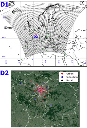
param-Figure 1. Overview of the coarse (D1 having 50 km resolution) and
local scale (D2, illustrated by the red rectangle having 4 km reso-lution) simulation domains. In D2, the city of Paris in located in the area enclosed by the purple line. Circles correspond to sites of the local air-quality monitoring network (AIRPARIF), with red for urban, blue for suburban and black for rural.
eters of model configuration to help improve regional-scale climate change assessments.
2 Materials and methods
2.1 Meteorological and air-quality models’ setup The IdF region is located at 1.25–3.58◦ east and 47.89– 49.45◦ north with a population of approximately 11.7 mil-lion, more than 2 million of which live in the city of Paris (Fig. 1). The area is situated away from the coast and is characterized by uniform and low topography, not exceeding 200 m a.s.l.
In order to simulate air quality in the study region, we em-ploy a dynamical downscaling approach: at first the IPSL-CM5A-MR global circulation model (Dufresne et al., 2013) is used to derive projections of the main climate drivers
(tem-perature, solar radiation etc.) using the RCP-4.5 data set of greenhouse gas emissions (van Vuuren et al., 2011). Global climate output is downscaled with the Weather Research and Forecasting (WRF) mesoscale climate model (Skamarock and Klemp, 2008) over Europe at a 0.44◦ horizontal res-olution grid (details on these simulations can be found in Kotlarski et al., 2014). For the purpose of the sensitivities presented in the paper we also employ meteorology driven by ERA reanalysis data at two resolutions; 0.11◦and 0.44◦ (Vautard et al., 2013). The vertical resolution of the meteo-rological input consists of 31σ-p layer extending to 500 hPa. Pollutant concentrations at the global scale are mod-eled with the LMDz-INCA chemistry model (Hauglustaine et al., 2004, 2014) forced with RCP-4.5 emissions. These concentration fields are downscaled at the regional scale with the CHIMERE (2013a version) off-line chemistry-transport model (http://www.lmd.polytechnique.fr/chimere) in two steps: initially at 0.44◦resolution grid (∼50 km) over Europe and subsequently at 4 km resolution over the IdF re-gion. The nesting scheme is presented in Fig. 1. CHIMERE is a cartesian mesh-grid model including gas-phase, solid-phase and aqueous chemistry, biogenic emissions modeling with the MEGAN model (Guenther et al., 2006), dust emis-sions (Menut et al., 2005) and resuspension (Vautard et al., 2005). Gas-phase chemistry is based on the MELCHIOR mechanism (Lattuati, 1997) which includes more than 300 reactions of 80 gaseous species. The aerosols model species are sulfates, nitrates, ammonium, organic and black carbon and sea-salt (Bessagnet et al., 2010), and the gas–particle partitioning of the ensemble Sulfate/Nitrate/Ammonium is treated by the ISORROPIA code (Nenes et al., 1998) imple-mented on-line in CHIMERE. CHIMERE has been bench-marked in the past in a number of model inter-comparison experiments (see Menut et al., 2013a, and references therein). For the reference run at the urban scale (hereafter REF), we use the same model setup as in Markakis et al. (2014): the modeling domain has a horizontal resolution of 4 km and consists of 39 grid cells in the west–east direction, 32 grid cells in the north–south direction and 8σ-p hybrid vertical layers from the surface (999 hPa) up to approximately 5.5 km (500 hPa) with the surface layer being 25 m thick. The con-figuration of the reference run represents the best compro-mise between local-scale emission data and the high compu-tational demand of a long-term simulation at fine resolution. 2.2 Climate and emissions
simulations at the global scale. The choice of the RCP-4.5 was dictated by the availability of chemical simulations on the regional scale.
The regional-scale simulations for the present-time (2010) employ an emission database developed in the framework of the ECLIPSE (Evaluating the Climate and Air Quality Im-pacts of Short-Lived Pollutants) project (Klimont et al., 2013, 2015) implementing emission factors from GAINS (Amann et al., 2011). Present-time emissions (as areas sources) are compiled by the International Institute for Applied Systems Analysis (IIASA) and regarding Europe, they include the re-sults of the work undergone in the UNECE Convention on Long-Range Transboundary Air Pollution (CLRTAP). The emission estimates are available at a 0.5◦×0.5◦ resolution grid.
Present-time (2008) emission estimates for the IdF region are also available in hourly basis over a 1 km resolution grid. This emission inventory is compiled by the Île-de-France en-vironmental agency and combines a large quantity of city-specific information (AIRPARIF, 2012) based on a bottom-up approach. The spatial allocation of emissions is either source specific (e.g., locations of point sources) or com-pleted with proxies such as high-resolution population maps and a detailed road network. The inventory includes emis-sions of CO, NOx, Non-methane volatile organic compounds (NMVOCs), SO2, PM10 and PM2.5with a monthly, weekly and diurnal – source specific – temporal resolution. Emis-sions from point sources are inputted as area emisEmis-sions in the model, and the grid cells containing those sources adopt a vertical distribution across model layers which varies in time-dependent from several meteorological variables such as temperature and wind inputted in a plume-rise algorithm (Scire et al., 1990). Consequently the distribution of emis-sions among different activity sectors reveals that in the IdF region the principal emitter of NOx, on annual basis, is the road transport sector (50 %), for NMVOCs the use of solvents (50 %) and for fine particles the residential sector (37 %). The raw data of the 1 km resolution emissions were aggregated to the 4 km resolution modeling grid.
2.3 Data and metrics for model evaluation
Model results from the different sensitivity runs are com-pared against observational data for O3, NO, NO2and PM2.5. Pollutant concentrations measured at 29 sites of the air-quality network of AIRPARIF (17 urban, 4 suburban and 8 rural) are compared to first-layer modeled concentrations on the grid-cells containing the corresponding monitor sites. To benchmark model performance we use the skill scoreS, which is based on the equations of Mao et al. (2006): S=1
2 1− BIAS MGE + MGE RMSE , (1)
where MGE represents the absolute mean gross error and RMSE the root mean square error. A skill score close to 1
is indicative of an unbiased model with no significant errors present, but in the case of biased results this rating masks the information on the magnitude of the bias and the corre-sponding error. For this reason, alongsideS, we employ the mean normalized bias (MNB) and mean normalized gross er-ror (MNGE) regarding ozone evaluation and the mean frac-tional bias (MFB) and mean fracfrac-tional error (MFE) regarding PM2.5(EPA, 2007).
We extract these metrics from the daily concentration val-ues and not the decade average bearing in mind that this is not typical for runs forced by climate simulations but for opera-tional forecast evaluation. We should note here, that it is rea-sonable to expect lower scores than those achieved in opera-tional forecast analysis due to the presence of climate biases (Colette et al., 2013; Menut et al., 2013a). As in Markakis et al. (2014) we aim to evaluate our simulations by utilizing metrics that are time averaged on a scale finer than a clima-tological one.
2.4 Description of the sensitivity simulations
Through a number of test cases we study the ability of the model to predict present-time decadal air-quality with re-spect to emission and meteorological input as well as the CTM’s horizontal and vertical resolution. For that purpose we conduct five sets of 10-year-long simulations (1996– 2005) over a 4 km resolution grid covering the IdF region (see Table 1). In all our comparisons we use as a measure of sensitivity of modeled ozone and PM2.5the absolute dif-ference between the mean of daily averaged concentrations (|1c|) as well as the absolute change in the skill scoreS. For ozone we also compare the MNB, MNGE and for PM2.5the MFB and MFE. All scores are calculated to represent an av-erage of all urban, suburban or rural stations. For PM2.5for which only observations from urban stations are available we represent the results for summer, winter and in annual basis of urban stations.
in-Table 1. Parameterization of the different sets of simulations presented in the paper. Changes with respect to the REF case are marked in
bold. Changes with respect to a simulation other than REF are marked in italics.
Annual emission Air-quality Emission inventory Emission post- climate/reanalysis Number of layers totalsa model resolution resolution processingb meteorology and resolution in air-quality model
REF AIRPARIF 4 km 4 km Bottom-up RCP-4.5 (0.44◦) 8 REGc ECLIPSE 0.5◦ 0.5◦ Top-down RCP-4.5 (0.44◦) 8
Sensitivity simulation
ERA05 AIRPARIF 4 km 4 km Bottom-up ERA (0.44◦) 8
ERA01d AIRPARIF 4 km 4 km Bottom-up ERA (0.11◦) 8
VERT AIRPARIF 4 km 4 km Bottom-up RCP-4.5 (0.44◦) 12 ANN ECLIPSE 4 km 4 km Bottom-up RCP-4.5 (0.44◦) 8 POSTe ECLIPSE 4 km 4 km Top-down RCP-4.5 (0.44◦) 8 AVERf ECLIPSE 4 km 0.5◦ Top-down RCP-4.5 (0.44◦) 8 aThe resolution of the emission inventory of AIRPARIF is 1 km (aggregated to 4 km for the purpose the local simulations) and the ECLIPSE inventory 50 km. bTemporal, vertical allocation and chemical speciation.
cThis simulation is used as boundary conditions for all local-scale simulations. dThe ERA01 simulation is compared with the ERA05, not with the REF. eThe POST simulation is compared with the ANN, not with the REF.
fThis is not a standalone simulation. Concentrations modeled at 4 km resolution with the POST run are averaged spatially to match the cells of REG (0.5◦resolution simulation). AVER results are compared to REG to quantify the effect of model resolution and with POST to quantify the effect of the resolution of the emission inventory.
terpolating the 0.44◦ resolution meteorology over the 4 km resolution CHIMERE grid adds a source of uncertainty in modeled pollutant concentrations, but due to the flat topog-raphy of the area and as shown in previous research studies in the same region, increasing the resolution of the meteo-rological input does not improve model performance (Menut et al., 2005; Valari and Menut, 2008). To study the impact of the resolution of the input meteorology here, we conduct a second sensitivity run where meteorological input stems from a WRF simulation using ERA40 reanalysis data over a finer resolution mesh with grid spacing of 0.11◦(ERA01) and compare with the ERA05 run.
The third sensitivity test addresses the issue of the CTM’s vertical resolution (VERT). A previous sensitivity analy-sis conducted with the same air-quality model showed only small changes in modeled ozone and PM10 concentrations over the IdF region due to increase in the CTM’s vertical res-olution (Menut et al., 2013b). On the other hand, Menut et al. (2003) showed that vertical diffusivity was one of the most influential parameters to the observed daily peak concentra-tions of ozone for a typical summertime episode in IdF. Here, we undertake a similar analysis but in a climate modeling framework, where enhanced meteorological bias is expected. VERT implements a 12 verticalσ-p layers instead of 8. The major difference between the two configurations (REF vs. VERT) is not the number of layers but the depth of the first model layer, which is reduced from 20 to 8 m in VERT. We note that because the WRF meteorology (resolved in 31 lay-ers) is interpolated to the CTM’s vertical grid, technically, increasing the number of vertical layers in CHIMERE from 8 to 12 will result in a refinement of the meteorological input used for the chemical simulations as well.
The fourth sensitivity case estimates the discrepancy in modeled ozone and PM2.5 concentrations between two
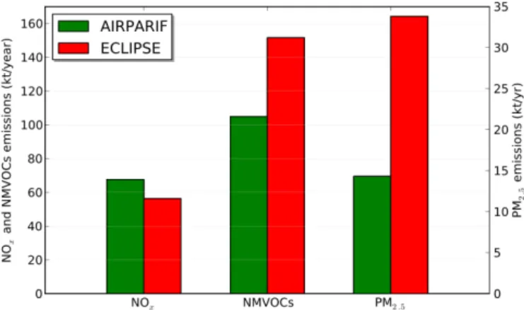
allo-Figure 2. Domain-wide annual emissions of NOx, NMVOC (left-axis) and PM2.5(right-axis) from the local (bottom-up) and the re-gional (top down) inventory (summed across the vertical column).
cate wintertime emissions from wood-burning. We note here, that the interest of comparing the two emission inventories is strictly to quantify the added value of implementing local-scale information in city-local-scale climate studies and not by any means to compare qualitatively the two data sets. It should be made clear that the ECLIPSE data set is not meant to ac-curately represent emissions at such fine scales.
In the fifth sensitivity case we study the impact of the post-processing methodology e.g., the process followed in order to split the annual emission totals into hourly emis-sion fluxes for all the species and vertical layers required by the air-quality model. Menut et al. (2012a) showed that model performance improves when time-variation profiles developed on the basis of observations are applied for the temporal allocation of emissions instead of the EMEP co-efficients. Mailler et al. (2013) found that model results are highly sensitive to the coefficients used for the vertical dis-tribution of emissions. Makar et al. (2014) investigated the response of modeled concentrations to the refinement of the spatial and temporal allocation of input emissions and found that the model was as sensitive to these improvements as to the vertical mixing parameterization. Also they conclude that the temporal distribution of emissions in particular, could be very important in stable urban atmospheres and that this sensitivity is reduced with increased mixing conditions. For our test emission totals must match between the two emis-sion data sets. We compile a new emisemis-sion data set (POST) where the ECLIPSE annual totals are spatially (both hori-zontally and vertically) and temporally downscaled on the 4 km-resolution IdF grid. This procedure is based on coeffi-cients extracted from the ECLIPSE post-processed inventory which, in turn, derive from the EMEP model. Comparing be-tween the POST and ANN runs (Table 1) we can model the impact on pollutant concentrations of integrating a bottom-up approach in regional emission modeling.
Finally the impact of model horizontal resolution is a cru-cial issue for air-quality modeling. Regarding urban ozone,
there are plentiful studies on the effect of model resolu-tion refinement with an overall tendency to show improve-ment of the model’s quality when increasing resolution from about 30–50 to 4–12 km (Arunachalam et al., 2006; Cohan et al., 2006; Tie et al., 2010; Valari and Menut, 2008). On the other hand, reports are scarce for fine particles: Punger and West (2013) show that increasing the resolution from 36 to 12 km improved the 1 h daily maximum concentrations but not the daily average, Stroud et al. (2011) reported bet-ter agreement of fine particles of organic origin with mea-surements from a modeling exercise at a 2.5 km resolution domain over a 15 km resolution domain, while Queen and Zhang (2008) also show improvement but their results in-clude the effect of increasing the resolution of the meteoro-logical input as well. Valari and Menut (2008) showed that the impact of the resolution of emissions on modeled con-centrations of ozone may be higher than the model resolution itself. This question has not yet been raised in the framework of climate-driven atmospheric composition modeling at the local scale. In our study we disentangle the impact of the res-olution of the emission data set from the effect of model reso-lution itself by conducting two more tests. In the first test we employ the 0.5◦resolution simulation (REG hereafter) from which all aforementioned simulations take their boundary conditions. We also compile the AVER database which uses as a starting point the modeled concentrations at 4 km res-olution from the POST run spatially averaged over the 0.5◦ grid-cells of the REG resolution mesh. REG vs. AVER (see Table 1) can provide information on the influence of model resolution while comparing AVER against POST provides the sensitivity to the resolution of the emission inventory.
3 Model evaluation
3.1 Evaluation of present-time meteorology
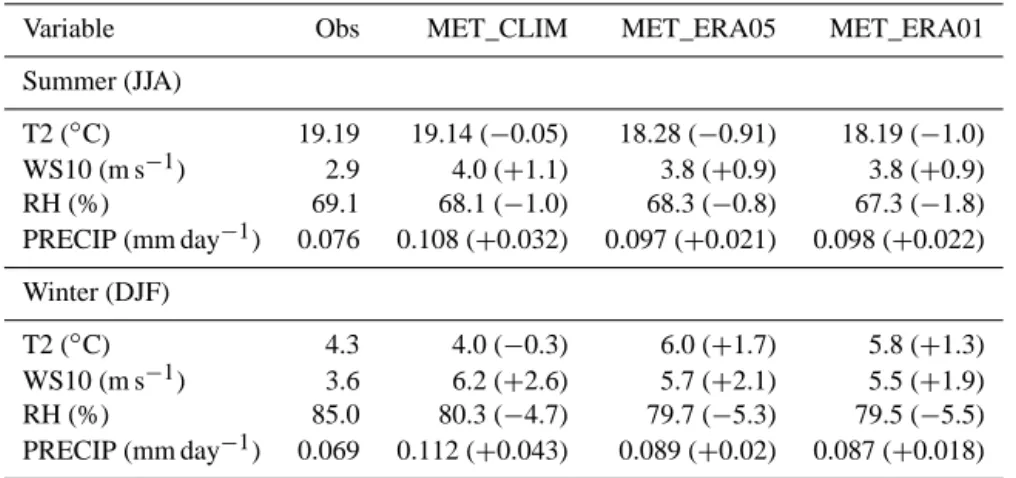
There are three WRF simulations involved in the study: (i) climate-model-driven meteorology downscaled from a global-scale climate model (MET_CLIM); (ii) meteorology from reanalysis data sets at 0.5◦resolution (MET_ERA05) and (iii) meteorology downscaled from reanalysis data at 0.11◦(MET_ERA01). In this section we present a short eval-uation of these data sets comparing model results against surface observations from seven meteorological monitoring sites existing in the domain. We note here, that from these monitors, only one is located inside the highly urbanized city of Paris. A thorough evaluation of the reanalysis data set in Europe may be found in Menut et al. (2012b).
Table 2. Observed and modeled daily average meteorological variables over the Île-de-France region. MET_CLIM data set stems from a
climate model and MET_ERA05, MET_ERA01 from reanalysis data at 0.5 and 0.1◦resolution, respectively. Absolute model bias is given in parenthesis.
Variable Obs MET_CLIM MET_ERA05 MET_ERA01
Summer (JJA)
T2 (◦C) 19.19 19.14 (−0.05) 18.28 (−0.91) 18.19 (−1.0)
WS10 (m s−1) 2.9 4.0 (+1.1) 3.8 (+0.9) 3.8 (+0.9)
RH (%) 69.1 68.1 (−1.0) 68.3 (−0.8) 67.3 (−1.8)
PRECIP (mm day−1) 0.076 0.108 (+0.032) 0.097 (+0.021) 0.098 (+0.022)
Winter (DJF)
T2 (◦C) 4.3 4.0 (−0.3) 6.0 (+1.7) 5.8 (+1.3)
WS10 (m s−1) 3.6 6.2 (+2.6) 5.7 (+2.1) 5.5 (+1.9)
RH (%) 85.0 80.3 (−4.7) 79.7 (−5.3) 79.5 (−5.5)
PRECIP (mm day−1) 0.069 0.112 (+0.043) 0.089 (+0.02) 0.087 (+0.018)
MET_ERA05 meteorology especially during the winter pe-riod. Such a bias, consistent with previous studies (see e.g., Jimenez and Dudhia, 2012 for WRF or Vautard et al., 2012 for other models), is expected to enhance pollutants’ dis-persion and lead to less frequent stagnation episodes. The bias is stronger for the MET_CLIM data set than for the MET_ERA05. A systematic wet bias in both summertime and wintertime precipitation is observed for the two data sets. This can significantly reduce PM concentrations through rain scavenging (Fiore et al., 2012; Jacob and Winner, 2009). MET_ERA05 fields provide a better representation of pre-cipitation especially in wintertime where the bias is reduced by a factor of more than 2 compared to MET_ CLIM. Sum-mertime temperature is adequately represented in the climate data set, whereas a wintertime weak cold bias (−0.3◦C) is observed. A strong hot bias during the winter is found for the reanalysis meteorology. A warmer climate can increase ozone formation through thermal decomposition of PAN re-leasing NOx (Sillman and Samson, 1995). RH is generally well represented in both cases.
Finally we notice that the finer resolution reanalysis data set (MET_ERA01) is not able to reduce the observed domain-wide biases of the coarse meteorological run with the exception of specific locations such as the Montsouris station in Paris where the bias in wintertime precipitation and wind speed bias is reduced by 22 and 40 %, respectively.
3.2 Evaluation of the reference simulation (REF)
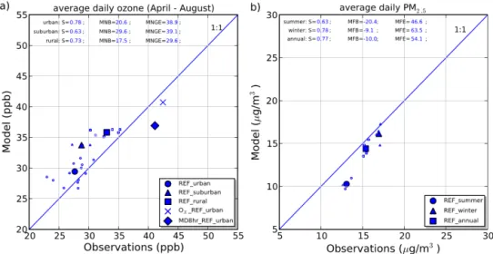
Mean modeled daily surface ozone and the daily maximum of 8 h running means (MD8hr) are compared against surface measurements in urban, suburban and rural stations (Fig. 3a). The results presented are averaged over the ozone period (April–August). We also use odd oxygen Ox=O3+NO2− 0.1×NOx(Sadanaga et al., 2008) as an indicator of the effi-ciency of the model to represent photochemical ozone
build-up. Contrary to O3, the concentration of Oxis conserved dur-ing the fast reaction of ozone titration by NO, and is therefore a useful metric for the evaluation of the photochemical ozone build-up by ruling out titration near high NOxsources (Vau-tard et al., 2007).
The model performs well in the urban areas capturing the mean daytime ozone levels (bias+1.8 ppb), while Oxis also accurately represented with an underestimation of only 4.1 %, illustrating the efficiency of the model to reproduce both daytime formation and titration of urban ozone. The bias in daytime average is smaller and less than 1 ppb. The Ox bias in daily averages is similar to the daytime one, sug-gesting underestimation of nighttime titration. This is consis-tent with other studies using CHIMERE (Szopa et al., 2009; Van Loon et al., 2007; Vautard et al., 2007). Model bench-mark ratings show a high skill score (0.78) while MNB and MNGE are+20.6 and 38.9, respectively.
We observe an overestimation of mean daytime suburban ozone (+5 ppb). The small bias in Ox (+0.6 ppb) suggests that the problem stems from the representation of local titra-tion and more specifically daytime titratitra-tion; the daily average ozone bias drops to+3.9 ppb while Ox is accurately repre-sented in this case (−0.2 ppb). Suburban stations present the lowest skill score (0.63) compared to urban and rural. Model performance over rural stations is adequate, with an over-estimation in mean daily ozone of 8.2 % (bias= +2.8 ppb) and a good skill score (0.73). The two major downwind loca-tions in the IdF domain which present the lowest biases (less than 0.1 and 1.1 ppb for the southwest and northeast direc-tions, respectively). The bias of the daytime average reaches
+2.1 ppb.
Figure 3. (a) Scatter plots and scores of daily average ozone concentrations at urban, suburban and rural stations from the REF simulation.
Odd oxygen (Ox)and daily maximum values at urban locations are also shown. textbf(b) daily average PM2.5concentrations in wintertime (DJF), summertime (JJA) and on annual basis over urban stations.
highlighting model sensitivity to accumulated errors (Valari and Menut, 2008). Modeled peak concentrations are particu-larly sensitive to temperature compared to the daily averages as shown in Menut at al. (2003). This could also be due to the fact that 4 km is still an insufficient model resolution.
The evaluation of PM2.5(Fig. 3b) shows a good represen-tation of daily average levels during wintertime where the highest annual concentrations are presented (bias less than 1 µg m−3). In annual basis the bias is also small while a larger underestimation is predicted for the summertime sea-son (bias=2.8 µg m−3). The latter can be due to underesti-mation of summertime emission fluxes (resuspension emis-sions are not considered in our simulations) and underesti-mation of secondary organic aerosols forunderesti-mation (Hodzic et al., 2010; Markakis et al., 2014; Solazzo et al., 2012). The overestimation in wind and precipitation also contributes to the observed PM underestimation. Wintertime and annual statistics show a high skill score. Interestingly, in wintertime and in the annual basis, the site located in downtown Paris presents the lowest bias (<0.3 µg m−3). Overall the results indicate that the fine-scale setup is able to predict the main patterns of ozone and fine particle pollution in the area.
4 Sensitivity cases
4.1 Sensitivity to climate-model-driven meteorology (REF vs. ERA05)
This case study estimates the discrepancy between an air-quality model run where regional meteorology is downscaled with WRF from reanalysis data (ERA05) and a simulation where meteorology is downscaled from a global-scale cli-mate model (REF). The wet bias in MET_CLIM
meteorol-ogy is significantly reduced with meteorolmeteorol-ogy from reanal-ysis data (Sect. 3.1). This is expected to have a significant role in the modeled PM concentrations. Another influential factor is the colder bias found in summertime temperature in the MET_ERA05 data set. This could lead to decreased reaction rates, less biogenic emissions and consequently to less ozone. The lower bias in 10 m wind speed under MET_ ERA05 is bound to increase surface concentrations through reduced dispersion. We also compare the average modeled boundary layer height (PBL) for the summer and winter pe-riods between the two data sets: PBL is reduced by 5 and 12 %, respectively, in summer and winter (not shown) when reanalysis data are used instead of climate model output. This may result in less dilution of emissions, and therefore higher surface concentrations for primary emitted species, such as PM and NOx.
Comparing the results of the two air-quality model runs for ozone (Fig. 4a and Table 3) we find only a small sensitiv-ity to using meteorology from a climate model or reanalysis data over all three types of monitor sites (|1c| ∼1 ppb or 3.4 %). The small improvement of model performance with the reanalysis data set (ozone decreases through higher NOx emissions following the PBL scheme described above) is due to the fact that titration is more realistically represented in ERA05 (the difference is Oxbetween the two runs is negli-gible). The response of urban daily maximum values to the meteorological data set is also negligible (|1c| =0.1 ppb or 0.3 %).
Figure 4. Scatter plots and scores for the sensitivity test on climate-model-driven meteorology for ozone and PM2.5.
Table 3. Absolute difference (and percentage in parenthesis) between daily averaged ozone (ppb) and PM2.5(µg m−3)from two climate-forced air-quality runs. The most influential factor for each sensitivity test is marked in bold.
Ozone Urban Suburban Rural
Climate meteo (REF vs. ERA05) 1.0 (3.4 %) 1.1 (3.2 %) 0.9 (2.5 %)
Meteo. resolution (ERA05 vs. ERA01) 0.2 (0.6 %) 1.4 (4.3 %) 0.3 (0.8 %)
Vertical resolution (REF vs. VERT) 0.3 (1.2 %) <0.1 (0.2 %) <0.1 (1.5 %)
Annual emis. totals (REF vs. ANN) 0.8 (2.5 %) 1.1 (3.2 %) 0.3 (1.0 %)
Emission post-proc. (ANN vs. POST) 1.9 (6.4 %) 0.1 (0.4 %) <0.1 (0.02 %)
Emission resolution (POST vs. AVER) 2.8 (8.3 %) 0.7 (1.9 %) 0.2 (0.5 %)
Model resolution (AVER vs. REG) 1.7 (4.7 %) 0.5 (1.4 %) 0.2 (0.5 %)
PM2.5 Summer Winter Annual
Climate meteo (REF vs. ERA05) <0.1 (0.05 %) 3.1 (17.6 %) 1.4 (9.4 %)
Meteo. resolution (ERA05 vs. ERA01) 0.3 (3.4 %) 1.3 (6.8 %) 0.6 (4.0 %)
Vertical resolution (REF vs. VERT) <0.1 (0.3 %) 0.5 (2.2 %) <0.1 (0.2 %)
Annual emis. totals (REF vs. ANN) 4.1 (33.0 %) 6.6 (33.8 %) 5.5 (31.9 %)
Emission post-proc. (ANN vs. POST) 3.4 (24.8 %) 4.5 (18.3 %) 0.2 (0.7 %)
Emission resolution (POST vs. AVER) 2.1 (20.3 %) 7.1 (30.0 %) 4.3 (24.2 %)
Model resolution (AVER vs. REG) 0.4 (4.1 %) 0.4 (1.9 %) 0.7 (0.5 %)
run (|1c| =1.4 µg m−3or 9.4 %). The use of the reanalysis data leads to a strong overestimation of wintertime concen-trations (Fig. 4b), which stems directly from the reduction (and improvement) of precipitation by a factor of 2 in the meteorology from reanalysis. This leads to the conclusion that the small bias observed in the REF simulation during wintertime (Fig. 4b) could be due to model error compen-sation such as unrealistically high precipitation and possible inhibition of vertical mixing or overestimation of wintertime emissions. The scores suggest a slight deterioration in model performance when passing from meteorology from a climate model to reanalysis meteorology in both winter and summer but improvement when focusing on the annual statistics.
We conclude that using climate-model-driven meteorol-ogy has a small impact on modeled ozone, whereas larger sensitivity is observed for wintertime PM2.5levels due to the accuracy of modeled precipitation.
4.2 Sensitivity to the resolution of the meteorological input (ERA01 vs. ERA05)
def-Figure 5. Scatter plots and scores for the sensitivity test on the resolution of meteorology for ozone and PM2.5.
initely higher than over urban or rural sites. Ox change at the suburban area (not shown) is much weaker compared to ozone (|1c| ∼0.5 ppb or 1.2 %) showing that the increase in the resolution of meteorology has an impact on the represen-tation of ozone titration leading to improved model perfor-mance. The skill score over suburban sites increases by 9 % while NMB improves by 22 % from 26.1 in ERA05 to 20.3 in ERA01. Interestingly, the response of suburban ozone to the resolution of the meteorological input is the strongest mod-eled sensitivity for this variable amongst all studied cases.
Weak sensitivities are modeled for PM2.5(Table 3) during summertime (|1c| =0.3 µg m−3or 3.4 %) and on annual ba-sis (|1c| =0.6 µg m−3or 4 %), but stronger during the win-ter season (|1c| =1.3 µg m−3or 6.8 %). In fact, wintertime statistics suggest that model bias actually increases with the refinement of the meteorological grid as a consequence of the reduced modeled precipitation (less scavenging), and PBL by 20 % (weaker dispersion) in MET_ERA01 compared to the climate-model-driven meteorology (Sect. 3.1). Again, this points to the same error compensation scheme described in the REF vs. ERA05 comparison (Sect. 4.1).
We conclude that the resolution of the meteorological in-put has a small impact on modeled ozone, while moder-ate sensitivity is observed for suburban ozone and winter-time PM2.5. Never the less, this result could reflect the lo-cal area’s characteristics (flat terrain, situated away from the coast) confirming previous studies (Menut et al., 2005; Valari and Menut, 2008). In regions with more complex topography or those close to the coast, the resolution of the meteorolog-ical input could have a profound effect on the simulated me-teorological conditions (Leroyer et al., 2014). We note here that the refinement in the resolution of the meteorological model from 0.5 to 0.1◦may not be sufficient for the CTM to simulate noticeable concentration responses. For example Leroyer et al. (2014) (see also references therein) observed
that substantial changes in vertical and horizontal transport in an urban environment occurred mostly in the transition from resolutions of 2.5 to 1 km and even higher (250 m).
4.3 Sensitivity to the resolution of the CTM’s vertical grid (REF vs. VERT)
This study addresses the impact of the resolution of the CTM’s vertical mesh and more specifically of the thickness of the first CTM layer, on modeled ozone and PM2.5 con-centrations (Fig. 6). Mean daily ozone is practically insensi-tive to the refinement of the vertical mesh at the urban, sub-urban and rural areas (Table 3). Similarly, maximum ozone at the urban area changes by only 0.5 ppb (1.4 %) with in-creased bias in the VERT run. Changes in summertime and annual modeled PM2.5 concentrations are also small, while the wintertime daily average shows some weak sensitivity (|1c| =0.5 µg m−3or 2.2 %). Scores are hardly affected.
Figure 6. Scatter plots and scores for the sensitivity test on the CTM’s vertical resolution for ozone and PM2.5.
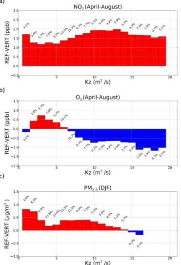
NO2 concentrations increase with the refinement of the first vertical layer of the CTM for all vertical mixing con-ditions (Fig. 7a). However it is only under low vertical mix-ing (1< Kz<5 m2s−1) that ozone sensitivity becomes pos-itive (Fig. 7b). Under stronger turbulence (Kz>5 m2s−1), the 12-layer setup leads to higher first-layer NO2 concentra-tions (stronger titration) leading to negative values for ozone sensitivity (such conditions account for the 93 % of the sim-ulated period). On the other hand, the refinement of the ver-tical mesh primarily affects NO2deposition rates which ac-celerate by 14.3 % but leaving ozone deposition rates unaf-fected. We may assume that under low mixing conditions, the increased deposition rate of NO2slows down the increase in NO2concentration due to the emission effect and dynamical processes become more influential than titration. As a result the surface layer is enriched in ozone by getting mixed with air from higher atmospheric layers (Menut et al., 2013b).
For almost the entireKz range, PM2.5concentrations in-crease with VERT (Fig. 7c). This is due to the fact that emis-sions are released in smaller volumes as discussed above. On the other hand, also here the refinement of the vertical reso-lution of the CTM enhances deposition rate. These two con-flicting effects explain the small impact of the CTM’s vertical resolution on PM2.5concentrations.
We conclude that both ozone and PM2.5 sensitivities to the refinement of the vertical mesh are small. Our analysis suggests that in both cases, this is the result of two compet-ing processes, either titration against vertical mixcompet-ing (ozone) or emission vs. deposition (PM2.5). Although in the Île-de-France area (low topography), the overall effect is insignifi-cant, it may not be the case in other regions with more com-plex topography.
4.4 Sensitivity to the annual emission totals (REF vs. ANN)
Figure 7. Difference in average daily simulated NO2(a), ozone (b) and PM2.5 (c) concentrations between VERT (12 vertical layers) and REF (8 vertical layers) at urban areas per range of Kz (bins of 1 m2s−1). Positive differences indicate that the refined vertical mesh leads to increased pollutant concentration and vice versa. The occurrence of sensitivity values within eachKzrange is also pro-vided.
concentrations modeled with the ANN run are significantly higher than those modeled with the REF run (Fig. 8b). Win-tertime bias in ANN reaches+5.8 µg m−3showing that fine particle emissions from the ECLIPSE inventory are overes-timated (see also Fig. 2). The main source of primary win-tertime PM2.5 emissions over the IdF region as well as in Paris in the ANN run is wood burning (see discussion in Sect. 2.4), which is unrealistic for a city like Paris and stems directly from the use of the population proxy to spatially al-locate national totals over the finer scale. This is consistent with the fact that the summertime bias in the ANN run is much lower (+1.4 µg m−3). In fact, in this case the ANN bias is even smaller than the REF bias (−2.8 µg m−3)enhancing our hypothesis that summertime fine particle emissions in the AIRPARIF inventory are underestimated (see also Sect. 2.1).
The skill score in REF is higher than in ANN in wintertime and lower in summertime.
We conclude that ozone sensitivity to the annual emission totals is low but strong for fine particles.
4.5 Sensitivity to emission post-processing (ANN vs. POST)
Here we use identical annual totals but two different meth-ods for their vertical and temporal allocation to obtain hourly fluxes over the 4 km-resolution domain as well as different matrices for their chemical speciation. The ANN data set uses the AIRPARIF bottom-up approach, whereas the EMEP methodology is applied to the POST data set. To compile the ANN inventory we had to extract the post-processing coef-ficients of the bottom-up inventory and apply them on the ECLIPSE annual totals. This procedure, however, was not emission-source-sector-oriented, and this inconsistency def-initely affects model results. On the other hand, the post-treatment of the (sectoral) raw emissions in large-scale ap-plications are typically based on sectoral coefficients that do not link back to the same quantified emissions either. For ex-ample, in the regional application used this study (REG), the sectoral ECLIPSE raw emissions quantified in SNAP level are treated with the respective sectoral coefficients that stems from the EMEP inventory having a very different synthe-sis of sub-SNAP sources from that of ECLIPSE. Therefore when we compare ANN with POST we consider that what we observe is the bias of this inconsistency in regional mod-eling. The question raised is the following: what is the benefit of adopting bottom-up post-processing for regional-scale air-quality modeling?
The effect on ozone concentrations over the urban area is considered moderate (|1c| =1.9 ppb or 6.4 %) (Fig. 9a and Table 3). Model bias is reduced from+4.5 ppb in POST to
Figure 8. Scatter plots and scores for the sensitivity test on the annual emission totals for ozone and PM2.5.
Figure 9. Scatter plots and scores for the sensitivity on the post-processing (temporal analysis and chemical speciation) technique applied
on the annual emission totals for ozone and PM2.5.
zones are located and assigns only 70 % of the total NOx emissions over Paris in the first model layer.
Another important piece of information id the diurnal vari-ation of emissions. Although the time scale of a climate-forced run largely exceeds the hourly basis, we aim to illus-trate how important the choice of the diurnal patterns can be to the final modeled concentrations. Figure 10a shows the average diurnal variation of modeled and observed urban ozone for ANN and POST (for the modeled fields we use the grid cells of the monitoring sites). The two downscal-ing approaches compared here, apply different diurnal pro-files on emissions to provide hourly fluxes. Between 10:00 and 15:00 LT, ANN underestimates ozone concentrations due to too much NO emissions, enhancing titration, and this is maximized in the local peak (15:00 LT) where NO concen-trations are overestimated by a factor of 2 (not shown). The
Figure 10. Mean diurnal variation of (a) ozone concentrations
aver-aged over the April–August period and (b) wintertime PM2.5 con-centrations in the urban area.
Modeled PM2.5sensitivity is significant for both summer and wintertime (|1c| =3.4 µg m−3or 24.8 % and 4.6 µg m−3 or 18.3 % respectively) (Table 3). POST wintertime bias is al-most 2 times higher than ANN (Fig. 9b). This is because the coarse resolution annual post-processing coefficients weight towards allocating more of the annual emissions into the win-ter period significantly influenced by the residential sector emissions which are overstated in the ECLIPSE inventory. A late afternoon peak is modeled with ANN accounting for the traffic emissions, whereas PM2.5evening levels modeled with the POST run (after 20:00 LT) are related to the residen-tial heating activity (Fig. 10b).
What we can conclude is that in a climate-forced air-quality framework, the model response for daily average ozone by 6.2 % is rather small considering the significant dif-ferences that the two post-processing approaches prescribe for the vertical distribution of emissions and their diurnal variation. Fine particle concentrations are much more sen-sitive to the applied emission post-processing technique. We note here, that recent work has pointed out that the sensitiv-ity of modeled concentrations the spatiotemporal resolution of the emission inventory is model-dependent (Makar et al., 2014).
4.6 Sensitivity to the emission inventory resolution (POST vs. AVER)
Here, we quantify the effect of the resolution of the emis-sion input. Results show that in the urban areas, this sen-sitivity is the most influential amongst all tests presented in this paper with ozone changes reaching 2.8 ppb or 8.3 % (Fig. 11a). The change in daily average Ox is smaller but comparable (|1c| =1.2 ppb or 2.9 %), suggesting that ozone titration is not the only model process that is affected by the increase in the resolution of the emission data set. The skill score and MNB improve significantly in the POST run (Ta-ble 3). Ozone precursors’ emissions from urban sources are mixed with the lower emissions from the surrounding subur-ban and rural areas inside the large cells of the coarse mesh-grid (AVER). This leads to lower titration rates and there-fore, higher ozone levels. Therefore the increase in the reso-lution of the emission input leads to a reduced positive bias from+7.3 ppb (AVER) to+4.5 ppb (POST). AVER overes-timates ozone peaks by 0.8 ppb while POST underesoveres-timates them by−1.2 ppb. The sensitivity of ozone concentration at the hour of the afternoon peak is linked to NOx concentra-tion at the same hour, which reaches a local maximum due to the evening rush hour (see also Sect. 4.5). Suburban and rural ozone is less sensitive than urban (|1c| =0.7 ppb), with scores practically unchanged (Table 3).
Fine particle concentrations are also very sensitive to the resolution of the emission input, especially in winter-time (|1c| =7.1 µg m−3or 30 %), with higher concentrations modeled with the refined emission inventory in POST (Ta-ble 3). As is also the case with ozone, this is because in the coarser inventory represented here by AVER, emissions in the high emitting areas in the city are smoothed down and di-luted when averaged with emissions of the less poldi-luted outer areas.
We conclude that the resolution of the emission input is the most influential factor from all the studied cases, even more than model resolution itself. PM2.5showed higher sen-sitivity than ozone concentrations. The non-linear nature of ozone chemistry suggests that it is important for the ozone precursor emissions to be concentrated correctly to the high emitting areas such as the urban centers.
4.7 Sensitivity to model horizontal resolution (AVER vs. REG)
Figure 11. Scatter plots and scores for the sensitivity test on the resolution of the emission inventory for ozone and PM2.5.
titration rates. Suburban and rural ozone has low sensitivity to model resolution (|1c| =0.5 ppb or 1.4 % and 0.2 ppb or 0.5 % respectively) because photochemical build-up occurs at larger time and space scales compared to titration, and the refinement of the model grid does not increase performance. This confirms the results in Markakis et al. (2014). The effect on modeled PM2.5is very small with concentrations slightly higher over the finer mesh grid as a result of the lower pri-mary emissions in REG.
We may conclude that the benefit of increasing the CTM’s resolution is insignificant for both ozone and PM2.5 espe-cially taking into account the large refinement attempted here (0.5◦to 4 km).
5 Sources of error in regional climate-forced atmospheric composition modeling
In this paper we utilize simulations at two spatial scales: at the urban scale over a grid of 4 km resolution using the AIRPARIF bottom-up inventory of anthropogenic emissions (REF) and a regional-scale run at 0.5◦resolution where emis-sions stem from the ECLIPSE top-down inventory (REG). Both realizations implement identical climate-driven mete-orology (at 0.44◦ resolution) and an 8-layer vertical mesh; therefore, they are susceptible to the same sources of error due to climate-model-driven meteorology, the resolution of the meteorological input and the resolution of the CTM’s ver-tical grid. However the remaining biases presented in Table 3 over urban areas e.g., the emissions resolution, the model horizontal resolution, the annual quantified fluxes and the post-processing method concern mainly the REG run. Re-garding ozone, REG has a positive bias of 9 ppb over the city of Paris while the bias of REF is only+1.8 ppb (Fig. 13a). The question we raise is “what are the main sources of
uncer-Table 4. The top row presents the coarse resolution application
(REG) model bias of the April–August average urban ozone and wintertime urban PM2.5. Subsequently, marked with italics the sig-nals – measured as the absolute concentration change from REG – of several refinements such as increase of resolution (model or emissions) and adaptation of annual quantified fluxes and post-processing of a bottom-up inventory. The individual signals sum up to the absolute bias found under the fine resolution simulation (REF).
Ozone (ppb) PM2.5(µg m−3)
REG (50 km) +9.0 +3.6
Model resolution −1.7 −0.4
Emissions resolution −2.8 +7.1
Annual emission totals −0.8 −6.6
Emissions post-processing −1.9 −4.5
REF (4 km) +1.8 −0.8
tainty in regional-scale climate-driven air-quality simulations and how these could be eliminated or at least reduced?”
With this study, we are able to identify the source of the excess of |1c| =7.2 ppb of ozone modeled with the REG run compared to REF (Table 4); 26.4 % (|1c| =1.9 ppb) is related to the post-processing of the annual emissions totals which are based on the EMEP factors, 11.1 % (|1c| =0.8 ppb) to the annual emission totals in the ECLIPSE inventory, 23.6 % (|1c| =1.7 ppb) to coarse model resolution and 38.9 % (|1c| =2.8 ppb) to the coarse resolu-tion of the ECLIPSE emission inventory.
an-Figure 12. Scatter plots for the sensitivity test on model resolution for ozone and PM2.5.
Figure 13. (a) Scatter plots of daily average ozone concentrations at urban, suburban and rural stations from the REF and REG simulations.
The odd oxygen (Ox)and daily maximum at urban locations is also shown. (b) Daily average PM2.5concentrations in wintertime (DJF), summertime (JJA) and on annual basis over urban stations.
nual totals alone but a more important gain would stem from the application of the AIRPARIF post-processing methodol-ogy. The added value from both of these factors would re-duce the positive bias of REG by 2.7 ppb. Even largest im-provement comes through the better spatial representation of ozone precursors emissions in the local emission inventory (|1c| =2.8 ppb) leading to more faithful titration process; Oxlevels are very close in REF and REG (Fig. 13a). It could therefore be argued that without increasing model resolution of which the gain would reach only 1.7 ppb, the REG sim-ulation would benefit significantly by simply integrating the aforementioned local-scale information.
The difference in modeled ozone between REF and REG is much smaller over the suburban area (|1c| =2.4 ppb), and the most influential factor to this difference is the annual
a strong wet bias reducing significantly PM2.5 concentra-tions (see also Sect. 3.1). Contrary to ozone, where infor-mation from the local scale improves in all cases model per-formance, the resolution of the emission inventory seems to deteriorate the modeling performance of PM2.5with an in-crease in the bias by 7.1 µg m−3. This only means that if the emission totals from ECLIPSE are used over Paris in the coarse REG application, then refining the resolution will only accumulate additional emissions in the city augment-ing the modeled concentrations. The remainaugment-ing features have also a positive effect; model resolution reduces the bias by 0.4 µg m−3, annual emission totals by 6.6 µg m−3and post-processing of the annual totals by 4.5 µg m−3. This essen-tially means that the regional realization cannot selectively incorporate any combination of local-scale features in order to improve performance as in the case of ozone. But the re-sults indicate that by simply integrating a bottom-up post-processing technique would result in an overall bias of the regional application of−0.9 µg m−3.
6 Conclusions
In the present paper we assess the sensitivity of ozone and fine particle concentrations with respect to emission and me-teorological input with a 10-year-long climate-forced atmo-spheric composition simulation at fine resolution over the city of Paris.
As a general observation, our study shows that overall ozone response is considered low to moderate, while PM2.5 concentrations were generally very sensitive for the pre-sented cases. The largest sensitivity in modeling the av-erage daily ozone concentrations was observed in the ur-ban areas primarily due to the resolution of the emission inventory (|1c| =2.8 ppb or 8.3 %) and secondly to the post-processing methodology applied on the annual emis-sion totals (|1c| =1.9 ppb or 6.2 %). These sensitivities are attributed to changes in the titration process. When post-processing coefficients were derived from the bottom-up AIRPARIF inventory instead of EMEP, too much ozone titra-tion takes place at the hour of the ozone peak, and the sen-sitivity of daily maximum reached its highest value among all the studied cases (|1c| =2.2 ppb or 5.8 %). It is interest-ing that despite the fact that ozone-precursor emissions are very different between the bottom-up and the top-down in-ventories, ozone sensitivity to the annual totals was shown to be very small (|1c| =0.8 ppb or 2.5 %). Also, modeled ozone is fairly insensitive to the use of climate model or re-analysis meteorology. Finally all cases of suburban and rural ozone both for average and maximum concentrations showed a sensitivity of less than 5 %.
Regarding PM2.5 concentrations, amongst all the pre-sented factors, the emissions related were those shown to be the most influential. The corresponding sensitivity to the use of annual emission totals from a top-down and a
bottom-up inventory reached 33 % in summer, 33.8 % in win-ter and 31.9 % for the daily average concentrations. This is connected to the downscaling methodology applied in the regional-scale totals of the ECLIPSE inventory; using pop-ulation as proxy for their spatial allocation, leads to overes-timation of particle emissions from wood-burning over the Paris area. Large sensitivity was also shown due to the reso-lution of the emission inventory (20.3 % in the summer, 30 % in the winter and 24.2 % in annual basis) because the coarser inventory smoothens the sharp emission gradients over the urban area leading to less primary emissions. Fine particle concentrations were also sensitive to the applied emission post-processing technique (22.1 % in summer and 16.7 % in winter). Only wintertime PM2.5concentrations were signif-icantly affected by the meteorological related sensitivities; by 17.6 % due to the use of meteorology from reanalysis in-stead of climate (mainly because the prescribed changes in modeled precipitation) and by 6.8 % due to refinement of the meteorological grid.
Both ozone and PM2.5are not very sensitive to the CTM’s vertical resolution (changes of less than 2.2 %). Nevertheless we provide evidence that this low sensitivity may be the re-sult of counteracting factors such as ozone titration, dry de-position and vertical mixing, too much dependent on local topography to be able to generalize for other regions. We also note the weak sensitivity of modeled concentrations to the in-crease in the CTM’s and the meteorological model’s horizon-tal resolution at least for the area and the range of resolutions studied here.
Excluding the sensitivities having the smallest impact (roughly less than 2 %, see Table 3) we observe a very consistent trend in ozone concentration: daily average and maximum ozone decrease as input data become more re-fined, namely passing from climate meteorology to reanal-ysis, increasing the resolutions of the horizontal and ver-tical CTM grid, of meteorology, of emissions and by us-ing bottom-up emissions and post-processus-ing instead of top-down. This decrease in ozone concentrations, from 2.5 up to 8.3 %, is observed mainly in the urban and suburban areas and in all cases stems from enhanced NOx emission fluxes in the surface-layer leading to titration inhibition. Trends and the underlying changes in emissions are highly variable for PM2.5with an increase in concentrations that may be as low as 2 % or as high as 30 % for climate meteorology and resolu-tion of the vertical mesh and also cases where concentraresolu-tion decreases in a wide range of values from 3 up to 34 % (annual emissions, model resolution) depending on the season.
urban areas. These biases could be taken into account in pol-icy relevant assessments.
The difference in modeled daily average ozone between the local and regional application over the urban areas (|1c| =7.2 ppb) is attributed to several sources of error: 38.9 % is related to the resolution of the emission inven-tory, 26.4 % stems from the post-processing of national an-nual emission totals, 23.6 % is due to model resolution (4 km or 0.5◦), and 11.1 % is associated with the annual emis-sions used as starting point for the compilation of the an-thropogenic emission data set. Although the greatest benefit in the regional-scale modeling seems to come through the increase in the resolution of the emission inventory, simpler actions may also be meaningful, such as the integration of the locally developed annual totals and the downscaling co-efficients derived from the existing bottom-up modeling sys-tems which, when combined, could reduce the bias of the re-gional application by 37.5 %. We note here that PM2.5levels in the urban regions are likely mostly controlled by primary emissions; increasing the emissions inventory resolution will concentrate the PM2.5emissions into a smaller spatial extent of the urban area (the reverse side of the artificial dilution is-sue taking place at coarse resolution); if the emissions totals are themselves biased high, then the resulting error will only become apparent at higher resolution. Therefore, the emis-sions resolution may show that the emisemis-sions totals are too high, and this only becomes apparent at high resolutions.
Regarding PM2.5modeling, our study shows that the re-gional realization cannot selectively incorporate any com-bination of local-scale features in order to improve perfor-mance as in the case of ozone. The simulation at the re-gional scale (REG) predicts an excess of 3.6 µg m−3 dur-ing wintertime compared to the fine-scale simulation (REF) showing a bias of −0.8 µg m−3, and this is attributed to the allocation of wood-burning emissions over the Paris area. Therefore, the most influential factor for PM2.5 mod-eling is the resolution of the emission input (REG-REF= +7.1 µg m−3). But the implementation of the refined emis-sion resolution of the local inventory alone would not ben-efit the regional simulation (which would increase the over-all bias to 10.7 µg m−3), neither the implementation of the annual emissions of the bottom-up inventory alone (REG-REF= −6.6 µg m−3)which would generate an overall neg-ative bias of 3 µg m−3. A simpler action would be to inte-grate the post-processing bottom-up technique (REG-REF= −4.5 µg m−3)giving an overall bias in REG of−0.9 µg m−3.
Acknowledgements. This work is supported by the ERA-ENVHEALTH project (grand agreement no 219337), co-funded by the European Commission under the 7th Framework Programme. The authors would also like to acknowledge Laurent Menut (LMD/Institute Pierre-Simon Laplace) and Augustin Colette (INERIS) for their insightful comments that helped improve this manuscript.
Edited by: K. Tsigaridis
References
AIRPARIF: Evaluation Prospective des emissions et des con-centrations des pollutants atmospheriques a l’horizon 2020 en Ile-De-France – Gain sur les emissions en 2015, Re-port available at: http://www.airparif.asso.fr/_pdf/publications/ ppa-rapport-121119.pdf (last access: 7 July 2015), 2012. Amann, M., Bertok, I., Borken-Kleefeld, J., Cofala, J., Heyes,
C., Höglund-Isaksson, L., Klimont, Z., Nguyen, B., Posch, M., Rafaj, P., Sandler, R., Schöpp, W., Wagner, F., and Winiwarter, W.: Cost-effective control of air quality and greenhouse gases in Europe: Modeling and policy applications, Environ. Model. Soft-ware, 26, 1489–1501, 2011.
Arunachalam, S., Holland, A., Do, B., and Abraczinskas, M.: A quantitative assessment of the influence of grid resolution on pre-dictions of future year air quality in North Carolina, USA, At-mos. Environ., 40, 5010–5026, 2006.
Beekmann, M. and Derognat, C.: Monte Carlo uncertainty anal-ysis of a regional-scale transport chemistry model constrained by measurements from the Atmospheric Pollution Over the Paris Area (ESQUIF) campaign, J. Geophys. Res., 108, 8559, doi:10.1029/2003JD003391, 2003.
Beekmann, M. and Vautard, R.: A modelling study of pho-tochemical regimes over Europe: robustness and variability, Atmos. Chem. Phys., 10, 10067–10084, doi:10.5194/acp-10-10067-2010, 2010.
Bessagnet B., Seigneur, C., and Menut, L.: Impact of dry deposi-tion of semi-volatile organic compounds on secondary organic aerosols, Atmos. Environ., 44, 1781–1787, 2010.
Brasseur, G. P., Jeffrey, T. K., Muller, J.-F., Schneider, T., Granier, C., Tie, X., and Hauglustaine, D.: Past and future changes in global tropospheric ozone: impact and radiative forcing, Geo-phys. Res. Lett., 25, 3807–3810, 1998.
Cohan, D. S., Hu, Y., and Russell, A. G.: Dependence of ozone sensitivity analysis on grid resolution, Atmos. Environ., 40, 126– 135, 2006.
Colette, A., Granier, C., Hodnebrog, Ø., Jakobs, H., Maurizi, A., Nyiri, A., Rao, S., Amann, M., Bessagnet, B., D’Angiola, A., Gauss, M., Heyes, C., Klimont, Z., Meleux, F., Memmesheimer, M., Mieville, A., Rouïl, L., Russo, F., Schucht, S., Simpson, D., Stordal, F., Tampieri, F., and Vrac, M.: Future air quality in Europe: a multi-model assessment of projected exposure to ozone, Atmos. Chem. Phys., 12, 10613–10630, doi:10.5194/acp-12-10613-2012, 2012.
Colette, A., Bessagnet, B., Vautard, R., Szopa, S., Rao, S., Schucht, S., Klimont, Z., Menut, L., Clain, G., Meleux, F., Curci, G., and Rouïl, L.: European atmosphere in 2050, a regional air quality and climate perspective under CMIP5 scenarios, Atmos. Chem. Phys., 13, 7451–7471, doi:10.5194/acp-13-7451-2013, 2013. Deguillaume, L., Beekmann, M., and Derognat, C.: Uncertainty
R., Bony, S., Bopp, L., Braconnot, P., Brockmann, P., Cadule, P., Cheruy, F., Codron, F., Cozic, A., Cugnet, D., de Noblet, N., Duvel, J.-P, Ethé, C., Fairhead, L., Fichefet, T., Flavoni, S., Friedlingstein, P., Grandpeix, J.-Y., Guez, L., Guilyardi, E., Hauglustaine, D., Hourdin, F., Idelkadi, A., Ghattas, J., Jous-saume, S., Kageyama, M., Krinner, G., Labetoulle, S., Lahel-lec, A., Lefebvre, M.-P., Lefevre, F., Levy, C., Li, Z. X., Lloyd, J., Lott, J., Madec, G., Mancip, M., Marchand, M., Masson, S., Meurdesoif, Y., Mignot, J., Musat, I., Parouty, S., Polcher, J., Rio, C., Schulz, M., Swingedouw, D., Szopa, S., Talandier, C., Terray, P., Viovy, N., and Vuichard, N.: Climate change projections us-ing the IPSL-CM5 Earth System Model: from CMIP3 to CMIP5, Clim. Dynam., 40, 2123–2165, 2013.
EPA: Guidance on the Use of Models and Other Analyses for Demonstrating Attainment of Air Quality Goals for Ozone, PM2.5 and Regional Haze, EPA -454/B-07-002, April, 2007. Fiore, A. M., Naik, V., Spracklen, D. V., Steiner, A., Unger, N.,
Prather, M., Bergmann, D., Cameron-Smith, P. J., Cionni, I., Collins, W. J., Dalsøren, S., Eyring, V., Folberth, G. A., Ginoux, P., Horowitz, L. W., Josse, B., Lamarque, J.-F., MacKenzie, I. A., Nagashima, T., O’Connor, F. O., Righi, M., Rumbold, S. T., Shindell, D. T., Skeie, R. B., Sudo, K., Szopa, S., Takemura, T., and Zeng, G.: Global air quality and climate, Chem. Soc. Rev., 41, 6663–6683, 2012.
Flagg, D. D. and Taylor, P. A.: Sensitivity of mesoscale model urban boundary layer meteorology to the scale of urban representation, Atmos. Chem. Phys., 11, 2951–2972, doi:10.5194/acp-11-2951-2011, 2011.
Forkel, R. and Knoche, R.: Regional climate change and its impact on photo-oxidant concentrations in southern Germany: Simula-tions with a coupled regional climate–chemistry model, J. Geo-phys. Res., 111, D12302, doi:10.1029/2005JD006748, 2006. Forkel, R. and Knoche, R.: Nested regional climate–chemistry
sim-ulations for central Europe, CR Geosci., 339, 734–746, 2007. Gilliland, A. B., Dennis, R. L., Roselle, S. J., and Pierce,
T. E.: Seasonal NH3 emission estimates for the eastern United States based on ammonium wet concentrations and an inverse modeling method, J. Geophys. Res., 108, 4477, doi:10.1029/2002JD003063, 2003.
Guenther, A., Karl, T., Harley, P., Wiedinmyer, C., Palmer, P. I., and Geron, C.: Estimates of global terrestrial isoprene emissions using MEGAN (Model of Emissions of Gases and Aerosols from Nature), Atmos. Chem. Phys., 6, 3181–3210, doi:10.5194/acp-6-3181-2006, 2006.
Hauglustaine, D. A., Hourdin, F., Jourdain, L., Filiberti, M.-A., Walters, S., Lamarque, J. F., and Holland, E. A.: Interac-tive chemistry in the Laboratoire de Meteorologie Dynamique general circulation model: Description and background tropo-spheric chemistry evaluation, J. Geophys. Res., 190, D04314, doi:10.1029/2003JD003957, 2004.
Hauglustaine, D. A., Balkanski, Y., and Schulz, M.: A global model simulation of present and future nitrate aerosols and their direct radiative forcing of climate, Atmos. Chem. Phys., 14, 11031– 11063, doi:10.5194/acp-14-11031-2014, 2014.
Hodzic, A., Jimenez, J. L., Madronich, S., Canagaratna, M. R., De-Carlo, P. F., Kleinman, L., and Fast, J.: Modeling organic aerosols in a megacity: potential contribution of semi-volatile and inter-mediate volatility primary organic compounds to secondary
or-ganic aerosol formation, Atmos. Chem. Phys., 10, 5491–5514, doi:10.5194/acp-10-5491-2010, 2010.
Hogrefe, C., Lynn, B., Civerolo, K., Ku, J.-Y., Rosenthal, J., Rosen-zweig, C., Goldberg, R., Gaffin, S., Knowlton, K., and Kin-ney, P. L.: Simulating changes in regional air pollution over the eastern United States due to changes in global and re-gional climate and emissions, J. Geophys. Res., 109, D22301, doi:10.1029/2004JD004690, 2004.
Im, I., Markakis, K., Koçak, M., Gerasopoulos, E., Daskalakis, D., Mihalopoulos, N., Poupkou, A., Tayfun, K., Unal, U., and Kanakidou, M.: Summertime aerosol chemic al composition in the Eastern Mediterranean and its sensitivity to temperature, At-mos. Environ., 50, 164–173, 2012.
Im, U., Markakis, K., Poupkou, A., Melas, D., Unal, A., Gerasopou-los, E., Daskalakis, N., Kindap, T., and Kanakidou, M.: The im-pact of temperature changes on summer time ozone and its pre-cursors in the Eastern Mediterranean, Atmos. Chem. Phys., 11, 3847–3864, doi:10.5194/acp-11-3847-2011, 2011.
Jacob, D. J. and Winner, D. A.: Effect of climate change on air qual-ity, Atmos. Environ., 43, 51–63, 2009.
Jimenez, P. A. and Dudhia, J.: Improving the Representation of Re-solved and UnreRe-solved Topographic Effects on Surface Wind in the WRF Model, J. Applied Meteorol. Climatol., 51, 300–316, 2012.
Katragkou, E., Zanis, P., Kioutsioukis, I., Tegoulias, I., Melas, D., Krüger, B. C., and Coppola, E.: Future climate change im-pacts on summer surface ozone from regional climate-air qual-ity simulations over Europe, J. Geophys. Res., 116, D22307, doi:10.1029/2011JD015899, 2011.
Kelly, J., Makar, P. A., and Plummer, D. A.: Projections of mid-century summer air-quality for North America: effects of changes in climate and precursor emissions, Atmos. Chem. Phys., 12, 5367–5390, doi:10.5194/acp-12-5367-2012, 2012. Klimont, Z., Kupiainen, K., Heyes, C., Cofala, J., Rafaj, P.,
Höglund-Isaksson, L., Borken, J., Schöpp, W., Winiwarter, W., Purohit, P., Bertok, I., and Sander, R.: ECLIPSE V4a: Global emission data set developed with the GAINS model for the pe-riod 2005 to 2050. Key features and principal data sources, avail-able at: http://eccad.sedoo.fr/eccad_extract_interface/JSF/page_ login.jsf (last access: 7 July 2015), 2013.
Klimont, Z., L. Hoglund, Heyes, Ch., Rafaj, P., Schoepp, W., Co-fala, J., Borken-Kleefeld, J., Purohit, P., Kupiainen, K., Wini-warter, W., Amann., M , Zhao, B., Wang, S. X., Bertok, I., and Sander, R.: Global scenarios of air pollutants and methane: 1990–2050, in preparation, 2015.
Knowlton, K., Rosenthal, J.vE., Hogrefe, C., Lynn, B., Gaffin, S., Goldberg, R., Rosenzweig, C., Civerolo, K., Ku, J.-Y., and Kin-ney, P. L.: Assessing Ozone-Related Health Impacts under a Changing Climate, Environ. Health Perspect., 112, 1557–1563, 2004.
Kotlarski, S., Keuler, K., Christensen, O. B., Colette, A., Déqué, M., Gobiet, A., Goergen, K., Jacob, D., Lüthi, D., van Meij-gaard, E., Nikulin, G., Schär, C., Teichmann, C., Vautard, R., Warrach-Sagi, K., and Wulfmeyer, V.: Regional climate model-ing on European scales: a joint standard evaluation of the EURO-CORDEX RCM ensemble, Geosci. Model Dev., 7, 1297–1333, doi:10.5194/gmd-7-1297-2014, 2014.