Lisboa, Portugal
Artificial Intelligence in Geospatial Analysis:
applications of Self-Organizing Maps in the context of
Geographic Information Science
A thesis submitted in partial fulfilment
of the requirements for the degree of
Doctor of Philosophy in Information Systems
by
Roberto André Pereira Henriques
Copyright by Roberto Henriques
Abstract
The size and dimensionality of available geospatial repositories increases every day, placing additional pressure on existing analysis tools, as they are expected to extract more knowledge from these databases. Most of these tools were created in a data poor environment and thus rarely address concerns of efficiency, dimensionality and automatic exploration. In addition, traditional statistical techniques present several assumptions that are not realistic in the geospatial data domain. An example of this is the statistical independence between observations required by most classical statistics methods, which conflicts with the well-known spatial dependence that exists in geospatial data.
Artificial intelligence and data mining methods constitute an alternative to explore and extract knowledge from geospatial data, which is less assumption dependent. In this thesis, we study the possible adaptation of existing general-purpose data mining tools to geospatial data analysis. The characteristics of geospatial datasets seems to be similar in many ways with other aspatial datasets for which several data mining tools have been used with success in the detection of patterns and relations. It seems, however that GIS-minded analysis and objectives require more than the results provided by these general tools and adaptations to meet the geographical information scientist‟s requirements are needed. Thus, we propose several geospatial applications based on a well-known data mining method, the self-organizing map (SOM), and analyse the adaptations required in each application to fulfil those objectives and needs. Three main fields of GIScience are covered in this thesis: cartographic representation; spatial clustering and knowledge discovery; and location optimization.
which is a geospatial-aware variant of SOM, was extended and implemented in the GeoSOM Suite tool, providing a useful and efficient framework for knowledge extraction and spatial clustering tasks. Using a different approach, a hierarchical SOM is proposed to explore and cluster geospatial datasets. Tests are performed using Lisbon‟s Metropolitan Area 2001 census data.
Resumo
O tamanho e a dimensionalidade dos repositórios de dados geoespaciais aumenta, a cada dia, exigindo das ferramentas de análise existentes um maior esforço para a extracção de conhecimento. A maioria destas ferramentas foram desenvolvidas num ambiente pobre em dados, razão pela qual aspectos como a eficiência, a elevada dimensionalidade e a exploração automática dos dados não são normalmente abordados nestas técnicas. A juntar a este facto, as técnicas estatísticas tradicionais apresentam diversas premissas que geralmente não são reais no contexto geoespacial. Um exemplo é a independência estatística entre os dados que é ponto de partida para a maioria dos métodos estatísticos clássicos, e que no caso dos dados geoespaciais não se verifica devido ao fenómeno de autocorrelação espacial.
Os métodos de inteligência artificial e data mining, que são menos dependentes de modelos, constituem assim uma alternativa na exploração e extracção de conhecimento de dados geoespaciais. Nesta tese, estudamos a possível adaptação de métodos gerais de data mining para analisar dados geoespaciais. As características destes dados parecem semelhantes em diversos aspectos aos dados não espaciais, para os quais diversas ferramentas de data mining têm sido usadas com sucesso na detecção de padrões e relações. Parece, contudo, que as análises típicas e os objectivos na maioria dos problemas da Ciência da Informação Geográfica, exigem uma adaptação dos métodos gerais que possam corresponder às expectativas dos cientistas geoespaciais. Assim, propomos nesta tese, diversas aplicações geoespaciais baseadas num método famoso em data mining, os mapas auto-organizáveis de Kohonen (SOM), e estudamos para cada caso as adaptações necessárias para garantir o cumprimento desses objectivos. Três áreas da Ciência da Informação Geográfica são abordadas nesta tese: a representação cartográfica; a descoberta de conhecimento e clustering espaciais; e a optimização de posicionamento.
Estados Unidos da América (baseado nos estados e nos condados), o cartograma da população portuguesa ou o cartograma da população mundial.
A segunda área da Ciência da Informação Geográfica abordada neste tese é a descoberta de conhecimento e clustering espaciais. Dois métodos são apresentados neste campo. O GeoSOM, que é uma adaptação do método SOM para lidar com dados geoespaciais, foi melhorado e implementado numa ferramenta (GeoSOM Suite) que permite de forma fácil e eficiente a extracção de conhecimento de dados geoespaciais. Usando uma abordagem diferente, é proposto um SOM hierárquico para exploração dos dados e criação de clustering temático. Como exemplo, diferentes análises foram feitas usando os dados censitários para a Área Metropolitana de Lisboa, referentes a 2001.
List of publications
List of published publications resulting from this thesis:
Henriques, R., F. Bacao and V. Lobo (2009). "Carto-SOM: cartogram creation using self-organizing maps." International Journal of Geographical Information Science 23(4): 483 -
511.
Henriques, R., F. Bacao and V. Lobo (2009). Spatial Clustering with SOM and GeoSOM Case study of Lisbon‟s Metropolitan Area. The Second International Conference on Advanced Geographic Information Systems, Applications, and Services International. GEOProcessing 2010
Henriques, R., F. Bacao and V. Lobo (2009). GeoSOM Suite: A Tool for Spatial Clustering. Computational Science and Its Applications - ICCSA 2009. 5592: 453-466.
Henriques, R., F. Bacao and V. Lobo (2009). UAV Path Planning Based on Event Density Detection. International Conference on Advanced Geographic Information Systems & Web Services, 2009. GEOWS '09.
Henriques, R., F. Bação and V. Lobo (2009). Cartograms, Self-Organizing Maps, and Magnification Control. Advances in Self-Organizing Maps: 89-97.
Henriques, R. and R. M. Rocha (2009). Sensor Network Deployment based on Data Variability. Proceedings of the 7th Conference on Telecommunications CONFTELE 2009, Santa Maria da Feira, Instituto de Telecomunicações.
Henriques, R., F. Bação and V. Lobo (2008). Planeamento de percursos em UAVs baseado em densidades de eventos. Jornadas do Mar 2008. O OCEANO - Riqueza da Humanidade, Escola Naval, Alfeite, Marinha Portuguesa.
Publications to be published:
Henriques, R., F. Bacao and V. Lobo "Exploratory geospatial data analysis using the GeoSOM suite." In submission.
Acknowledgements
Reaching this stage, I feel that the work presented in this thesis was not possible without the contribution of many persons and institutions though, of course, the final responsibility of this work remains mine. To them, I would like to express my great gratitude:
First, my supervisors, Professor Doutor Fernando Bação and Professor Doutor Victor Lobo, for their guidance, support, patience and friendship. They made me feel part of the team, and working with them was very compensating. May our collaboration and Chinese food dinners continue for many years.
The friendship and support from all my colleagues from LabNT. My special thanks to Paula Curvelo for all the discussions we had about this thesis.
To all the colleagues and Professors from ISEGI-UNL and IST who were somehow involved in this journey.
In addition, the reviewers of the different publications made from this work, which suggestions and comments allowed an improvement on the quality of this work.
Finally, to my family and friends for being my support in this thesis. To my wife Nucha, I must thank all the patience, love and help she gave me in this time. To my parents I must thank all the opportunities and belief they give me allowing the conclusion of this stage. To my brothers, parents in law and friends Paulo, Pedro and Carlos for their support and encouragement. Also, Thomas and Jutta, for their hospitality in Munster at the IFGI Spring School.
Acronyms
Acronyms are ordered by appearance in the text.
GIS Geographic Information Systems GISc Geographic Information Science SOM Self-Organizing Map
U-Mat Unified Matrix
UAV Unmanned Aerial Vehicle HSOM Hierarchical Self-Organizing Map SOAP Simple Object Access Protocol GPS Global Positioning System API Application Programming Interface GPX GPS Exchange Format
KML Keyhole Markup Language
VGI Volunteered Geographic Information
UCGIS University Consortium for Geographic Information Science NCGIA National Center for Geographic Information and Analysis AI Artificial Intelligence
CI Computational Intelligence HPC High Performance Computing TFL Tobler‟s First Law of Geography
MAUP Modifiable Areal Unit Problem
NUTS3 Nomenclature of Territorial Units for Statistics (level 3) ESDA Exploratory Spatial Data Analysis
EDA Exploratory Data Analysis DM Data Mining
GDM Geographic Data Mining BMU Best Matching Unit
PCA Principal Components Analysis MDS Multidimensional Scaling PCP Parallel Coordinate Plots ESOM Emergent Self-Organizing Maps GA Genetic Algorithms
STFM Spatial Temporal Feature Map KDD Knowledge Discovery and Data Mining LISA Local Indicators of Spatial Association ED Enumeration Districts
LMA Lisbon Metropolitan Area GUI Graphical User Interface MLP Multilayer Perceptron
Short index
1. Introduction ... 1
2. State of art ... 13
3. Building cartograms using the SOM ... 57
4. GeoSOM Suite: a tool for geospatial clustering ... 87
5. Hierarchical SOM for geospatial clustering ... 113
6. Mobile sensor network path definition problem ... 145
Index
Abstract ... iii
Resumo ... v
List of publications ... vii
Acknowledgements ... ix
Acronyms ... xiii
Short index ... xv
Index ... xvii
List of figures ... xxi
List of tables ... xxvii
1. Introduction ... 1
1.1. Context ... 2
1.1.1. GIScience & Geocomputation ... 4
1.2. The Problem ... 6
1.3. Objectives ... 9
1.4. Methodology ... 10
1.5. Thesis organization ... 11
2. State of art ... 13
2.1. Introduction ... 13
2.2. Self Organizing Maps ... 13
2.2.1. Overview ... 14
2.2.2. SOM algorithm ... 16
2.2.2.1. Sequential training ... 17
2.2.2.2. Batch Training ... 18
2.2.3. Parameterisation of the SOM ... 20
2.2.3.1. Size and dimension of the map ... 20
2.2.3.2. Topology, shape and initialisation ... 20
2.2.3.3. Number of iterations ... 22
2.2.4.2. Input space: non-linear projection ... 27
2.2.4.3. Output space: categorical maps ... 28
2.2.4.4. Output space: distance maps ... 30
2.2.4.5. Output space: frequency maps ... 31
2.2.4.6. Output space: temporal maps ... 32
2.2.4.7. Both spaces: linked maps ... 33
2.2.5. Quality of the SOM ... 35
2.2.6. Available Software ... 36
2.2.7. General considerations on SOM ... 37
2.2.8. Supervised variants of SOM ... 38
2.3. SOM & georeferenced data ... 40
2.3.1. Survey of SOM applied to the GIScience ... 41
2.3.1.1. Geovisualisation ... 43
A. Location visualisation ... 44
B. Context based visualisation ... 46
2.3.1.2. Spatial Clustering ... 47
A. Examples of geometric spatial clustering ... 48
B. Examples of implicit spatial clustering ... 50
C. Examples of explicit spatial clustering ... 50
2.3.1.3. Classification ... 53
2.3.2. Comparison of methods proposed in the literature ... 54
2.4. Discussion... 56
3. Building cartograms using the SOM ... 57
3.1. Introduction ... 58
3.1.1. Problem definition ... 59
3.2. Methods for building cartograms ... 60
3.2.1. Quantitative evaluation of cartograms ... 64
3.2.2. Global cartogram error ... 64
3.3. A New approach for building cartograms ... 65
3.3.1. Building Cartograms using SOM ... 65
3.3.2. Compensating for the magnification effect of SOM ... 69
3.3.3. Carto-SOM algorithm ... 71
3.4. Results ... 72
3.4.2. Sensitivity Analysis of Carto-SOM ... 74
3.4.2.1. Carto-SOM robustness test ... 74
3.4.2.2. Magnification effect ... 75
3.4.2.3. SOM parameters evaluation ... 76
A. Neighbourhood radius ... 76
B. Learning rate ... 77
C. Number of epochs ... 78
3.4.2.4. SOM dimension parameters ... 78
A. Number of units ... 78
B. Number of input data points ... 79
3.4.3. Comparison between Carto-SOM, Dougenik and Diffusion Cartograms ... 80
3.4.4. Related issues ... 83
3.5. Discussion... 86
4. GeoSOM Suite: a tool for geospatial clustering ... 87
4.1. Introduction ... 88
4.2. Related work ... 91
4.3. GeoSOM outline ... 92
4.4. Datasets used in this chapter ... 94
4.4.1. Squareville dataset... 94
4.4.2. Lisbon census ... 95
4.5. GeoSOM Suite tool ... 96
4.5.1. Views ... 97
4.5.2. Clustering in the GeoSOM Suite ... 100
4.5.3. Clustering spatial data ... 101
4.5.4. Combining multiple cluster in GeoSOM Suite ... 102
4.6. Case study: Lisbon‟s census ... 104
4.7. Discussion... 112
5. Hierarchical SOM for geospatial clustering ... 113
5.1. Introduction ... 113
5.2. Hierarchical SOM ... 116
5.2.1. Why use Hierarchical SOMs? ... 118
List of figures
Figure 1 - Self Organizing Map‟s output space (two-dimensional) and input space (three-dimensional). Blue circles represent the units of the SOM while the red circles represent the input patterns ... 15
Figure 2 – SOM training phase. A training pattern (red dot) is presented to the network and the closest unit is selected (BMU). Depending on the leaning rate, this unit moves towards the input pattern (represented by the red arrow). Based on the BMU and on the neighbourhood function, neighbours are selected on the output space (blue lightness represents the degree of neighbourhood). Neighbours are also updated towards the input pattern ... 16
Figure 3 - Voronoi regions. Space division where all the interior points are closer to the corresponding generator than to any other ... 19
Figure 4 – SOM topology: a) square topology with four neighbours and; b) hexagonal topology with six neighbours. The units considered neighbours of the black unit are presented in dark grey. All other units are in light grey ... 21
Figure 5 – Different SOM shapes implemented in SOM Toolbox using a square topology: a) sheet is the default SOM shape; b) cylinder shape and; c) toroid shape (Vesanto, Himberg et al. 2000)
... 21
Figure 6 – Comparison of the two-dimensional and spherical SOM (Wu and Takatsuka 2006) .. 22 Figure 7 - Learning rate functions... 23
Figure 8 - Neighbourhood functions. ... 24
Figure 9 - Taxonomy for SOM visualisation methods ... 25
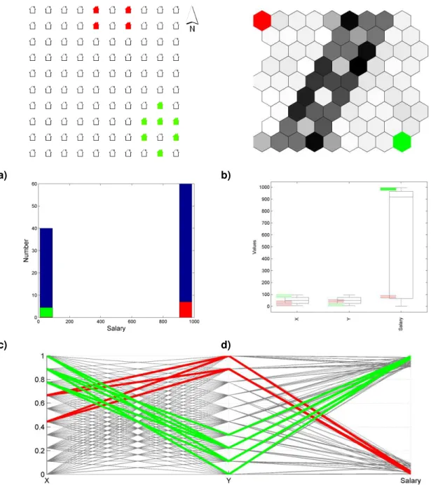
Figure 10 –Linear projections of the SOM‟s input space: a) Scatter plot of the SOM‟s input space using the unit‟s weights for the houses location (x and y coordinates) and the average salary; b)
scores from the two principal components obtained from the principal components analysis... 27
Figure 11 – Non-linear projections of the SOM‟s input space using Sammon mapping projection of the original three dimensions into a two-dimensional map ... 28
Figure 14 – Squareville variables histograms plotted on the SOM‟s output space. Black represents the x coordinate; grey represents the y coordinate and white represents the average
salary: a) SOM pie chart and; b) SOM bar chart ... 30
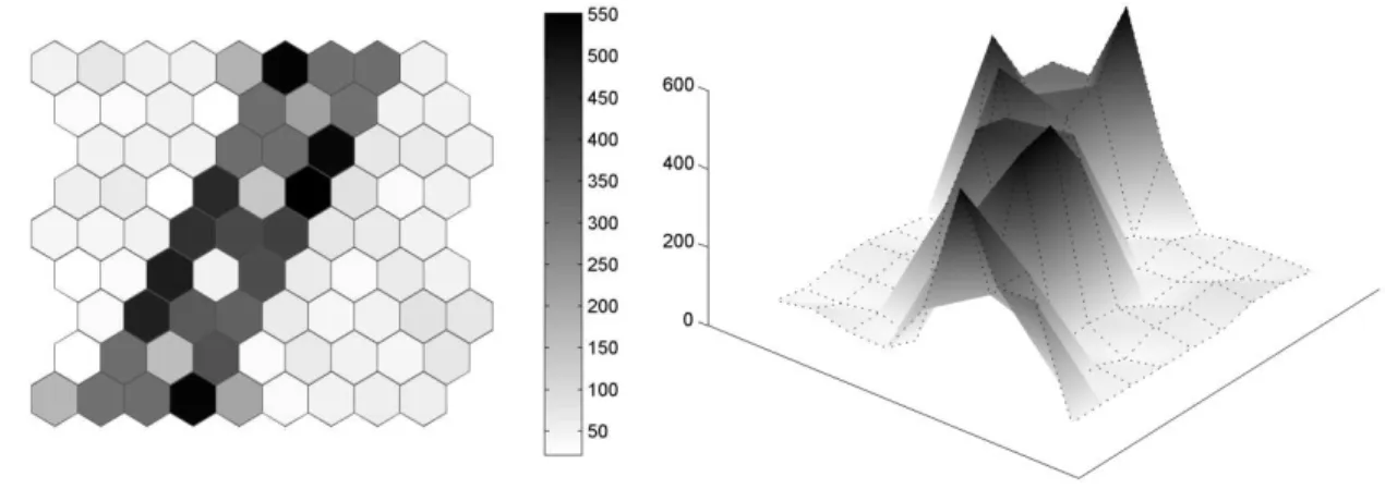
Figure 15 – U-matrix using Squareville data: a) two-dimensional U-matrix and; b) three-dimensional U-matrix ... 31
Figure 16 – Distance matrices using Squareville data: a) size coded distances; b) colour coded distances ... 31
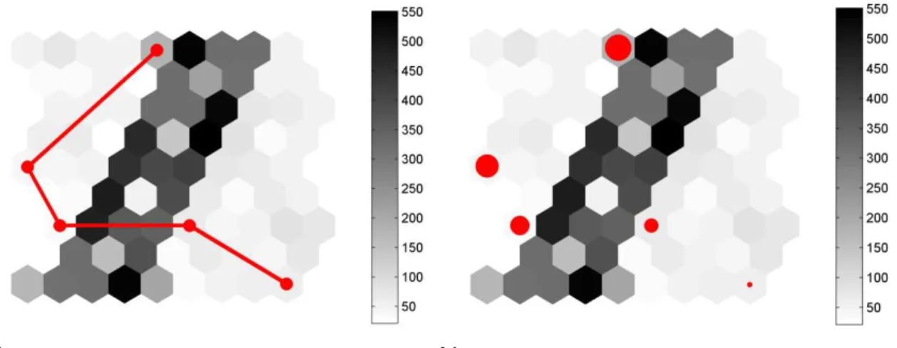
Figure 17 – Hits-map plot: a) using all data from Squareville, the size of the red hexagons represent the number of input patterns belonging to each unit and; b) using only input patterns where the average salary is less than 950, the size of the blue hexagons represent the number of input patterns belonging to each unit... 32
Figure 18 – Trajectories maps: a) trajectory map using a line to present the evolution and; b) comet map, in this case a comet like drawing presents the evolution (from larger to smaller circles) ... 33
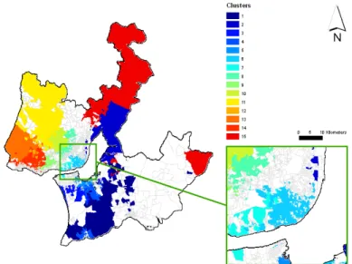
Figure 19 – Several linked space visualisations: a) geographical map, with classes obtained from the SOM; b) U-matrix presenting the same classes; c) combined histogram of the average salary for all the input patterns and input patterns from the selected classes; d) boxplot of the dataset presenting the distribution of the input patterns belonging to the classes and; e) parallel coordinate plot showing the classes‟ input pattern distribution ... 34 Figure 20 – Visualising the SOM in a geographic map. This example presents SOM based clusters of Lisbon Metropolitan Area, which will be further explained in chapter 4 ... 35
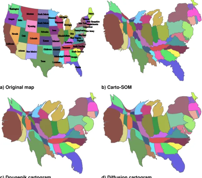
Figure 21 – Taxonomy for Self-Organizing Maps applications in GIScience ... 42 Figure 22 – Cartograms of USA population by state, using different cartogram building algorithms ... 63
Figure 23 – Proposed method example ... 67 Figure 24 – Rectangular shaped SOM superposed on a non-regular shaped dataset; a) random point creation based on a region feature; b) SOM units after training; c) Produced cartogram .... 68
Figure 25 – Input space nomenclature; a) SOM mapped in the input space; b) input space area definition: is the region area, and is the buffer area ... 68
Figure 29 – Carto-SOM error as a function of neighbourhood radius ... 77 Figure 30 – Carto-SOM error as a function of learning rate ... 77 Figure 31 – Carto-SOM error as a function of the number of epochs used ... 78 Figure 32 – Carto-SOM error as a function of the number of units ... 79 Figure 33 – SOM error as a function of the number of input data points ... 80 Figure 34 – Original map, Carto-SOM, Dougenik and diffusion cartograms of the artificial dataset ... 81
Figure 35 – Portuguese population cartograms using the Carto-SOM, Dougenik and Diffusion methods ... 81
Figure 36 – USA population cartograms using the Carto-SOM, Dougenik and Diffusion methods ... 82
Figure 37 – World countries population cartogram ... 84 Figure 38 – USA counties population cartogram ... 85 Figure 39 – Squareville (x and y represent the geographic coordinates while the colour represents
the average salary by house) ... 94
Figure 40 – Lisbon metropolitan area enumeration districts ... 95 Figure 41 – GeoSOM Suite architecture ... 96 Figure 42 – GeoSOM Suite window. From the left to the right, top to bottom: GeoSOM Suite main window (a) with a tree-list of available analysis, and the full dataset with all attributes; U-matrix (b) obtained using census data; geographic map (c) of Lisbon Metropolitan Area; and a boxplot (d) showing the distribution of two variables ... 97
Figure 43 – Dynamically linked views created by GeoSOM Suite (selection made in the U-matrix is in red); a) GeoSOM Suite main interface, with a tabular view of the dataset; b) boxplot view of the three variables; c) the average salary component plane, with a hit-map (in green) superimposed; d) the U-matrix; e) parallel coordinate plot of all the data and f) the geographic map ... 99
produced from the SOM. The average salary plane (c), the geographic map (d) and the parallel coordinate plot (e) are also presented (right column) showing the clusters ... 102
Figure 46 – Comparison between SOM and GeoSOM clustering. GeoSOM has the capability of detecting spatial contiguous clusters, while SOM produces global clusters. The selection in red shows one region with high average salary in the west part of the map. This region is not detected in the SOM due to the presence of another region with similar average salary in another region. a) Main GeoSOM window; b) U-matrix produced from a standard SOM; c) U-Matrix produced from GeoSOM; d) Average salary component plane of the standard SOM; e) Geographic map and f) parallel coordinate plot ... 103
Figure 47 – U-matrix (a) for Lisbon Metropolitan Area SOM and box plot (b) showing the outliers (red features both in U-matrix and in the boxplot) ... 105
Figure 48 – U-matrix (a) and component planes (b) for Lisbon Metropolitan Area dataset after exclusion of the outliers. The top row of component planes refers to the age of the building. The next row refers to the age of the residents, the third one the student status, the forth the achieved education levels, and the last the employment sector... 106
Figure 49 – U-matrix with outlines of some component plane hotspots. Areas of the component planes that have high values are shown with colours (one for each thematic group of variables) on top of the U-matrix. There are two areas where age (in green) plays a predominant role: on the right there is an area with many people over 65, and on the lower left an area with infants (under 13 years of age). There are three areas where education level (in blue) plays a predominant role: on the extreme right, upper left, and middle bottom, there are many people with tertiary education. Finally there are 5 areas (in red) where buildings have a well defined age structure: in the top right there are many old buildings (built before 1945), in the bottom right buildings built in the 60‟s (before 1970), in the top left, buildings of the 70‟s (before 1980), in the middle-left bottom the 80‟s (before 1990), and in the bottom left the 90‟s (before 2001) ... 107 Figure 50 – Component planes for the variables Id65 (a), E1945 (b) and E1970 (c) and Lisbon
map (d) showing the selection of the units with higher percentage of elder people ... 108
Figure 51 – U-matrix (a), parallel coordinate plot (b) and Lisbon Metropolitan Area map (c) with the highest percentage of buildings built before 1945‟ enumeration districts in red ... 109 Figure 52 – U-matrix obtained with GeoSOM for Lisbon‟s Metropolitan Area dataset after exclusion of outliers. The original cluster of old buildings detected by the standard SOM is mapped to the red units ... 110
Figure 53 – Oldest buildings cluster selected on the ED1945 component plane (a) and on the
Figure 54 – Clusters created for Lisbon‟s Metropolitan Area presented in the: a) U-matrix b) parallel coordinate plot of clustered units and c) Lisbon Metropolitan Area map ... 111
Figure 55 – HSOM taxonomy ... 119 Figure 56 – Types of hierarchical SOMs: a) agglomerative and; b) divisive ... 120 Figure 57 – Thematic HSOMs ... 121 Figure 58 – HSOMs based on clusters ... 122 Figure 59 – Static HSOMs: a) structure in which each unit will origin a new SOM and; b) structure in which a group of units will origin a new SOM ... 123
Figure 60 – Dynamic HSOMs ... 124 Figure 61 – Hierarchical SOM (HSOM) used. Labels a, b and c refer to different themes ... 127
Figure 62 – HSOM implementation in GeoSOM Suite. In this example, two SOMs are trained using buildings and population age data. An HSOM is parameterised using these two SOM‟s outputs (BMU coordinates and quantization error) and the geographical coordinates of each ED ... 129
Figure 63 – Lisbon metropolitan area enumeration districts ... 130 Figure 64 – Visualisation of U-Matrices. Outlier selection (in red) on the a) Standard SOM, and selection update on: b) HSOM; c) Lodgings; d) Buildings; e) Families; f) Age structure; g) Education level and; h) Employment ... 132
Figure 65 – Boxplot of all the variables used showing their distribution in the dataset (in grey). The black line connects the mean value of the selected EDs for each variable. The top graph has the variables grouped by themes, while in the bottom graph they are ordered by decreasing difference between the selection, and total average ... 133
Figure 66 – Visualisation of U-Matrices. Outlier selection (in red) on the b) HSOM, and selection update on: a) Standard SOM; c) Lodgings; d) Buildings; e) Families; f) Age structure; g) Education level and; h) Employment ... 134
Figure 67 –Bela Vista neighbourhood ... 135
Figure 68 – Selection (in red) of two EDs belonging to the Bela Vista: a) U-matrix from the
standard SOM and b) U-matrix created from the HSOM ... 135
Figure 71 – Selection of similar EDs (in red) to Bela Vista in the standard SOM: a) SOM U-matrix;
b) HSOM U-matrix; c) geographical map with EDs selection; d) Lodgings‟ U-matrix; e) Buildings‟ U-matrix; f) Families‟ U-matrix; g) Age structure U-matrix; h) Education level U-matrix and; i) Employment U-matrix ... 138
Figure 72 – Boxplot of all the variables used showing the distribution of the selected EDs. Variables were normalized using z-score (mean equals zero) ... 138
Figure 73 – Selection of similar EDs (in red) to Bela Vista in the HSOM: a) geographical map of
the Bela Vista selected ED, b) SOM U-matrix; c) HSOM U-matrix; d) Lodgings‟ U-matrix; e)
Buildings‟ U-matrix; f) Families‟ U-matrix; g) Age structure U-matrix; h) Education level U-matrix and; i) Employment U-matrix ... 139
Figure 74 – Geographic representation of the 150 clusters created using: a) standard SOM and; b) HSOM. Each cluster is represented by a unique colour. Since the two methods create different partitions, the colours are not comparable between the two solutions. However, for each solution the colour codes guarantee that similar clusters in the SOM share similar colours ... 140
Figure 75 – Modified quantization error for each standard SOM and HSOM, using only geographical coordinates, only aspatial variables, and using both ... 141
Figure 76 – Neighbourhood cluster ratio (ncr) calculated for k=1 to k=14. ncr gives the percentage
of total EDs sharing k spatial neighbours with the same cluster ... 142
Figure 77 – The ship simulator: a) fishing boats versus merchant ships behaviour b) initial distribution of the ships ... 149
Figure 78 – Benchmark methods: fixed locations and zigzag trajectories for the sensors ... 150 Figure 79 – Ship detection using an SOM based, fixed and zigzag UAV methods in a area of 10000x10000 meters, at for different instants: a) instant t; b) instant t+1; c) instant t+2 and; d)
instant t+3 ... 151
List of tables
Table 1 - Comparison table of SOM-based analysis in the GISc context ... 54
Table 2 - Best SOM parameters used in the Artificial, Portuguese and USA datasets ... 74
Table 3 - SOM parameters used to test input data points influence ... 75
Table 4 - Magnification factor ( ) variation ... 75
Table 5 - Variation of the neighbourhood radius ... 76
Table 6 - Variation on the learning rate ... 77
Table 7 - Variation on the number of epochs ... 78
Table 8 - Variation on the number of units used ... 79
Table 9 - Variation of the number of input data points ... 79
Table 10 - Keim error evaluation using different criteria on the various datasets ... 83
Table 11 - Variables used in the cluster analysis of LMA census ... 104
Table 12 - Comparison table of HSOM methods ... 127
1. Introduction
“Such systems [GIS] are basically concerned with describing the Earth‟s surface rather than analysing it. Or if you prefer, traditional 19th century geography reinvented and
clothed in 20th century digital technology” (Openshaw, Charlton et al. 1987).
“Techniques are wanted that are able to hunt out what might be considered to be localised patterns or „database anomalies‟ in geographically referenced data but without being told either „where‟ to look, or „what‟ to look for, or „when‟ to look” (Openshaw 1994).
1.1. Context
We live in a digital world. Nowadays data acquisition methods continuously record all sort of events occurring in the physical world. Improvements on both hardware and software technologies allow us to collect huge amounts of data, producing, every day, more complete, accurate and detailed pictures of human activity and interaction with the environment. All this torrent of data is being stored in ever increasing data warehouses.
These developments have increased the relevance of information in modern society, which in turn has led to even higher rate of information production developed in this area. It is a generally shared idea that information is an important resource in any organization. Possibly, the answer to many human/world problems may in fact depend on our ability to tap into this digital picture that we have of the world. However, organizations often collect raw data and produce sparse information but fail to create knowledge. A step further is needed, where this data/information is analysed, explored and converted into knowledge and ultimately used to solve problems and create value. Data Mining can be an important tool in bridging the gap between data and knowledge, through automated analysis which enables the extraction of knowledge from these databases (Hand, Smyth et al. 2001).
An important evolution has occurred in most databases, related with the global demand for a geospatial context, which forced the inclusion of space in these repositories. This
demand has been underlined by major technological advances leading to a new paradigm in the creation/use of contents. Major changes started around 2000, and were caused by factors such as:
the dot-com boom and the increase of broadband use;
the browsers‟ improvement in supporting new technologies such as SOAP and XML;
the fall in prices of data storage;
the changes in the way software developers and end-users use the Web (known as WEB 2.0 (O'Reilly 2005));
the creation of Web services and simplified APIs;
widespread use of low-cost position-aware devices such as GPS-navigation devices and cell phones.
The combination of these factors led to an increase in the number of people using the Web to create, assemble and disseminate geographic information. These new users have, in general, new needs and objectives in dealing with geospatial data and technologies. To deal with this new perspective, Turner (2006) proposes a new subfield in Geography, which he called Neogeography and defines it as the “set of techniques and tools that fall outside the realm of traditional GIS [Geographic Information Systems] (...). Where historically a professional cartographer might use ArcGIS, talk of (...)
projections, and resolve land area disputes, a neogeographer uses a mapping API1 like
Google Maps, talks about GPX2 versus KML3 and geotags his photos to make a map of his summer vacation”.
Goodchild called this new paradigm “volunteered geographic information” (VGI) and
defined it as “... a special case of the more general Web phenomenon of user generated content” (Goodchild 2007). Goodchild thinks that, although some quality issues must be
thought over carefully, these new sources of data can be useful to several applications such as military and commercial intelligence.
Some examples of the most common geospatial databases come from Earth Observation Satellites, census surveys and climate/environmental monitoring systems. Examples where the geospatial component has surfaced recently can be found in
1 API (application programming interface) is an interface that defines the ways by which an application program may request services from libraries and/or operating systems Wikipedia. (2009). "Application programming interface." Retrieved 19-08-2009, from http://en.wikipedia.org/wiki/Application_programming_interface.
2 GPX (GPS Exchange Format) is a XML data format for the interchange of GPS data (waypoints, routes, and tracks) between applications and Web services on the Internet Foster, D. (2009). "GPX: the GOS exchange format." Retrieved 19-08-2009, from http://www.topografix.com/gpx.asp.
customer/supply databases and product transaction repositories. Finally, some examples of Neogeography or VGI paradigm include geo-referenced data collected by position aware devices such as GPS receivers or cell phones or even wireless internet clients and cameras. This data is then uploaded by its creators to web based data repositories such as Google Maps (Google 2005), OpenStreetMap (OpenStreetMap 2004) or Wikimapia (Wikimapia 2006).
1.1.1.
GIScience & Geocomputation
Geographic Information Science (GISc or GIScience) is the scientific discipline that deals with the geospatial data. This discipline emerged 30 years after the creation of the first “modern” Geographic Information System (GIS) by Tomlinson in 1960, called Canada Geographic Information System (Tomlinson 1984; Tomlinson 1998). The term GISc was introduced by Goodchild (1992) and it is concerned with “the development and use of theories, methods, technology, and data for understanding geographic processes,
relationships, and patterns. The transformation of geographic data into useful
information is central to geographic information science” (UCGIS 2001). Mark (2003) on
the other hand, compiled a GISc definition by including the word geographic in an
Information Science definition due to Shuman (1992). In his proposal, “(Geographic) Information science is very difficult to define. (...) the field of (geographic) information
science, however, may be defined as one that investigates the properties and behaviour
of (geographic) information, how it is transferred from one mind to another, and optimal
means for making that transfer, in both natural and artificial systems. Finally,
(geographic) information science is concerned with the effects of (geographic)
information on people and on machines.”
A generally accepted definition of GIS (Geographic Information Systems) is given by the
National Center for Geographic Information and Analysis (NCGIA) which proposes“GIS as a system of hardware, software and procedures to facilitate the management, manipulation, analysis, modelling, representation and display of georeferenced data to solve complex problems regarding planning and management of resources” (NCGIA 1990).
with the amount, diversity and characteristics of modern geospatial data. As a reaction to the limits imposed by GIS software, Stan Openshaw proposes the “artificial intelligence paradigm as a core geographic skill” (Openshaw and Openshaw 1997).
The problems of using traditional statistical techniques in geospatial data derive from the following points (Atkinson and Martin 2000):
1) assumption of statistical independency of the data;
2) generalization of geography using global measures (e.g. average);
3) use of stationary models and;
4) use of model-based statistics for inference instead of letting data speak for themselves.
As an answer to these limitations, a new field called GeoComputation emerged. GeoComputation “is concerned with new computational techniques, algorithms, and paradigms that are dependent upon and can take advantage of high performance
computing (Openshaw 2000). In fact, Openshaw considers that GeoComputation is
founded on four technologies: the GIS for gathering data; artificial intelligence (AI) and computational intelligence (CI) providing the tools; computing power provided by high performance computing (HPC); and (geographic) science, which provides the philosophy or “raison d‟etre” (Openshaw 2000). To Openshaw, combining these factors makes GeoComputation the basis for a new paradigm for doing Geography. In fact, the letters
G and C in GeoComputation are purposely capitalized to distinguish this new field of
spatial analysis.
A different view is proposed by Couclelis who believes that “we have been doing geocomputation for years without realizing it”, under the quantitative geography umbrella
(Couclelis 1998). Her vision of GeoComputation is the “eclectic application of computational methods and techniques to portray spatial properties, to explain
geographical phenomena and to solve geographical problems” (Couclelis 1998).
Three main aspects make GeoComputation unique (Openshaw 2000). First, it is applied to geospatial data, assuming its distinctiveness. Many methods in quantitative geography were brought from other fields assuming no particularity exists in geospatial data. Secondly, GeoComputation uses an unparalleled computing power that provides new solutions and new ways of solving problems. Finally, GeoComputation requires a change in the way of thinking, because it is data-driven in the sense that knowledge is
deduced from data, instead of predefined or deduced by reasoning.
Longley et.al. (2005) assume GeoComputation as a synonym of GIScience, since they
both “suggest a scientific approach to the fundamental issues raised by the use of GIS and related technologies“.However, they adopted the idea that GeoComputation is more focused on the use of high-performance computers and artificial intelligence.
While agreeing in general with most of these views, in this thesis we assume that GeoComputation is a specialized branch of GIScience, which differs from the more general concepts of quantitative geography and GIS, in the sense that it is more focused on taking advantage of artificial intelligence techniques and computing power to develop new methods to solve GIScience problems.
1.2. The Problem
The amount of data in current geospatial repositories along with their high-dimensional nature requires a sophisticated set of analysis capabilities in order to extract new and unexpected patterns, trends, and relationships embedded in that data. General-purpose methods of data mining and knowledge discovery may not be suitable to geospatial data. This lack of suitability results from the fact that the spatial dimension cannot be seen just as two or three extra variables (such as x, y and z coordinates). It has been
said that geospatial data is particular and calls for special methods and analysis (Anselin 1989; Goodchild 1992; Openshaw 1999). These particularities fall into four major categories concerning aspects related to:
So, what is special in the attributes of geospatial data? First, the observations, the uncertainty and the error distribution are spatially dependent. This concept of spatial dependency was postulated in Tobler‟s first law (TFL) which states that “everything is related to everything else but near things are more related than distant things” (Tobler
1970). Directly related to the spatial dependency is the concept of spatial autocorrelation (Goodchild 1986). Spatial autocorrelation is the computational expression of spatial dependency. Another characteristic of geospatial data is spatial heterogeneity (Anselin 1988). Spatial heterogeneity is the property that makes each place on Earth unique, making design decisions successfully adopted in one region not always general and applicable in other regions (Goodchild 2008). These characteristics are important obstacles to standard premises used in traditional statistics.
As for distribution and dimensionality, geospatial data has, in general, a non-normal distribution and lies in a high-dimensional data space made up of two or three spatial dimensions and a potentially large number of aspatial dimensions. Also, this high-dimensional structure of data usually comprises redundancy and high correlation of some variables.
Data models and representation are also quite particular in geospatial data. The geographical space is continuous and infinite, but GIS requires the use of discrete representations. The delimitation of crisp boundaries to represent spatial continuous phenomena affects the accuracy and precision of data and consequently the analysis. One of these problems is known as the modifiable areal unit problem (MAUP) (Openshaw 1984). The MAUP consists on the fact that the variation in the spatial units used for aggregation will cause variation in statistical results. The outline of the area over which the description is obtained will influence critically the perception of the phenomena and if this aggregation is obtained at different scales, that perception will be even more biased. As an example, we can consider the criminality rate of Portugal. Assuming different aggregation levels such as Enumeration District, Civil Parish (Freguesia in Portuguese), Municipality (Concelho in Portuguese) or NUTS3, different
fallacy exists if one assumes that unemployed people are responsible for the crimes. Another particularity of geospatial data is related to its representation, which is usually made through compiled categorical layers, typically associated between them by spatial relationships.
Finally, the typical analysis performed with geospatial data has to consider the geospatial analyst‟s objectives and needs. For a geospatial analyst, space is the most important element, since the analysis is always spatially contextualized, and insights should primarily come from the specific spatial arrangements found. When exploring spatial data, the GIS scientist is searching for patterns, trends, and relationships spatially relevant. In fact, the most frequent type of analysis in geospatial data is exploratory. Exploratory spatial data analysis (ESDA) is a subset of exploratory data analysis (EDA) focused on the particular characteristics of geographic data (Anselin 1998). This set of techniques is based on user/data interaction allowing the detection of spatial patterns to build hypotheses on the dataset and evaluate its validity (Haining, Wise et al. 1998).
Data Mining (DM) is a step in the knowledge discovery process that automatically detects patterns in data (Fayyad, Piatetsky-Shapiro et al. 1996). Thus, Geographic Data
Mining (GDM) is a special type of data mining that seeks to apply standard data mining tools modified to take into account the special features of geospatial data and particular objectives and needs of GIS (Openshaw 1999; Harvey and Han 2001). Openshaw‟s perspective is that “new types of data mining tools that can handle the special nature of spatial information [are needed to] capture the spirit and essence of geographicalness that a GIS-minded data miner would expect to have available” (Openshaw 1999).
A slightly different perspective is held in (Bacao, Lobo et al. 2005) about how special
spatial data is, and consequently the necessity of new methods. In their view, most of the geospatial characteristics are not unique and may exist in aspatial secondary datasets. Secondary datasets, in opposition to primary datasets, are the sets of data not purposely collected for the analysis. Thus, geospatial data “can be considered a specific set of secondary data ... obtained with no specific analysis objectives in mind ... [with
some] characteristics similar [to] those observed in typical secondary data ... such as
the dependency issues ... selection bias, fuzziness, redundancy and even nonstationarity” (Bacao, Lobo et al. 2005). However, although machine learning methods
methods need to be made to deal with geographical perspective (Bacao, Lobo et al.
2005).
Bacao et.al. (2005) propose the adaptation of standard data mining tools whenever
possible, in opposition to the original GeoComputation proposal of developing new and specific methods to deal with geospatial data. Anyway, both visions agree that the use of standard of-the-box data mining tools in geospatial analysis will produce poor results
when compared with spatial aware methods.
The characteristics of geospatial datasets seem to be similar in many ways with other aspatial datasets for which several data mining tools exist to help in the detection of patterns and relations. It seems, however that GIS-minded analysis and objectives require more than the results provided by these general tools and possible adaptations to meet these conditions are needed.
This thesis attempts to answer the following research questions:
Is the SOM suitable for exploratory spatial data analysis? What are the possible applications of SOM in the GISc field?
What are the possible adaptations to the standard SOM algorithm to include geospatial reasoning in the analysis?
1.3. Objectives
The main objective of this thesis is to prove that data mining tools can be used to deal with geospatial data and provide examples of how they should be adapted to do so. The particular characteristics of this type of data and specific GIS-minded analysis can sometimes require adjustments in the general data mining methods, while in other cases minimal or no changes are necessary. These adjustments are dependent on the problem we are dealing with and on the expected results and analysis.
allows an improved understanding of the data. There have been several proposals to use SOM in the exploration of spatial data. One of SOM‟s most useful features is the density estimation capability. In fact, this ability can be of great usefulness in addressing several long-term problems in GIScience. In this thesis, the SOM is used in three of these GISc problems where density estimation is central: in the cartographic representation, in spatial data mining and in a particular case of the location/allocation problem.
The objectives of this thesis are:
1. to review SOM, focusing on some features that are familiar to GIS scientists like topology and visualisation techniques;
2. to review the use of SOMs in the geospatial context, comparing different approaches, results and available tools;
3. to examine more possibilities of adapting the SOM algorithm to the GIS-minded analysis;
4. to propose the use of the SOM to deal with several GIScience problems.
In line with the last objective, this thesis proposes:
a) a new method to create cartograms based on one geospatial variable;
b) an improved method to perform spatial clustering from high-dimensional datasets;
c) a new method to perform thematic spatial clustering from geospatial databases;
d) a new method to manage unmanned vehicles defining an optimised path to best cover a specific region.
1.4. Methodology
The approach we follow in this thesis starts by an in depth study of an artificial intelligence method, the SOM. This is a method widely used among data analysts with robust and reliable results. Also in the GIScience context, a growing number of proposals exist in the literature, e.g. (Agarwal and Skupin 2008). A survey of these
In our opinion, the use of SOM in the field of GISc could help in the solution of many GISs challenges and problems. From a review of the work done in the field, we identified three problems, stemming from three different areas in the GIScience field that could benefit from this particular method.
From the cartographic representation area, we test the possibility of using SOM to build cartograms. Concerning spatial analysis, we explored SOM-based methods (GeoSOM, Hierarchical SOM, and standard SOM), developing new techniques, improving others, and developing a user friendly software package that we made freely available. Finally, regarding a particular location/allocation problem, we tested SOM as the core of a method to handle the problem of path planning for a network of mobile sensors.
For each proposed problem we present a review, with special focus on the alternative methods used, benchmark datasets and evaluation measures. A detailed formulation of each problem is also presented, followed by a SOM-based method providing a possible solution. These methods are evaluated and compared with other methods using both fictional and real datasets.
1.5. Thesis organization
This thesis is organized as follows:
Chapter 2 presents the state of the art related to SOM. A review of the method is presented in the first part followed by a survey of SOM applications in the geospatial context.
Chapter 3 presents the first method developed in this thesis, where SOM is used to build cartograms in an approach called Carto-SOM. The basic idea of a cartogram is to distort a geographical map by substituting the geographic area of a region by some other variable of interest. The objective is to rescale each region according to the value of the variable of interest while keeping the map, as much as possible, recognizable.
designed to bridge the gap between clustering and the typical geographic information science objectives and needs, providing a user friendly environment. We believe that this tool can very useful to other researchers and practitioners.
In Chapter 5, we propose the use of Hierarchical SOMs to perform geospatial clustering. As we shall see, several characteristics of geospatial data make Hierarchical SOMs a natural choice for their analysis.
Chapter 6 introduces the fourth SOM based method developed. Here, SOM is used to deal with a real time location/allocation problem. The goal is to present a new method to define patrol paths for individual UAV (unmanned aerial vehicles), that compose a network of mobile sensors.
2. State of art
2.1. Introduction
The aim of this chapter is to provide an overview of the work done in the field of SOM and GeoComputation. We start by making an SOM overview, presenting its main properties and tools for exploration. Section 2.3 presents a survey of methods using SOM in the geospatial context.
2.2. Self Organizing Maps
multidimensional input data onto a lower dimension array of neurons (or units) is the Self-Organizing Map (SOM).
Self-Organizing Maps (SOMs), or Self-organizing feature maps (SOFMs) were first proposed by Tuevo Kohonen in the beginning of the 1980s (Kohonen 1982), and constitute the product of his work on associative memory and vector quantization. Since then there have been many excellent papers and books on SOM, but his book Self Organizing Maps,edited originally as (Kohonen 1995), and later revised in 1997 and 2001 (Kohonen 2001) is generally regarded as the main reference on the subject.
Kohonen's SOMs draw some inspiration from the way we believe the human brain works. Research has shown that the cerebral cortex of the human brain is divided into functional subdivisions and that the neural activity decreases as the distance to the region of initial activation increases (Kohonen 2001).
2.2.1.
Overview
SOM‟s basic idea is to map high-dimensional data onto one or two dimensions, maintaining the topological relations between data patterns. SOM‟s main objective is to “extract and illustrate” the essential structures in a dataset, through a map resulting from
an unsupervised learning process (Kaski and Kohonen 1996; Kaski, Nikkilä et al. 1998).
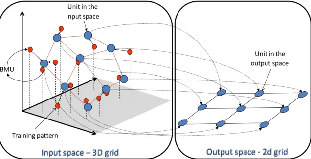
SOM is normally used as a tool for mapping high-dimensional data onto a one, two, or three dimensional discrete feature map. The grid formed by the units or neurons is what is usually referred to as the output space, as opposed to the input space, which is the original space where the data patterns lie (Figure 1).
The main advantage of SOM is that it allows us to have some idea of the structure of the data by observing the map. This is possible mainly due to preservation of topological relations, i.e., patterns that are close in the input space will be mapped, as far as
possible, to units that are close in the output space. The output space is usually 2-dimensional and in most implementations it is a rectangular grid of units (the grid can also be hexagonal) (Kohonen 2001). Single-dimensional SOMs are also common (e.g.
Gorricha and Lobo 2009). Using higher dimensional SOMs is rare because, although they pose no theoretical problem, the output space is difficult to visualise.
Figure 1 shows an example of a two-dimensional SOM with 3 x 3 units adapting to a three-dimensional input dataset.
Figure 1 - Self Organizing Map’s output space (two-dimensional) and input space (three-dimensional). Blue circles represent the units of the SOM while the red circles represent the input patterns
Each unit of the SOM, is represented by a vector mi=[mi1...,min] of dimension n, where n equals the dimension of the input space. In the training phase, a given training pattern x
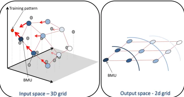
is presented to the network, and the closest unit is selected. This unit is called the best-matching unit (BMU) (Figure 1). The unit‟s vector values (synaptic weights in neural network jargon) and those of its neighbours are then modified in order to get closer to the data pattern x:
Equation I
Where is the learning rate at time t, and is the neighbourhood function
centred in unit c, and i identifies each unit. Both
and
decrease with timeOutput space - 2d grid
Input space
–
3D grid
Unit in the output space Unit in the
input space
BMU and on the neighbourhood function, neighbours are selected on the output space. These neighbours will also be updated, albeit less, towards the input pattern.
Figure 2 – SOM training phase. A training pattern (red dot) is presented to the network and the closest unit is selected (BMU). Depending on the leaning rate, this unit moves towards the input pattern (represented by the red arrow). Based on the BMU and on the neighbourhood function, neighbours are selected on the output space (blue lightness represents the degree of neighbourhood). Neighbours are also updated towards the input pattern
Independently of the quality of the training phase there will always be some residual distance between the training pattern and its representative unit. This difference is known as quantization error. This value is used to measure the accuracy of the map‟s representation of data. Section 2.2.5 presents a deeper explanation on the quality of the SOM.
2.2.2.
SOM algorithm
The SOM algorithm can be easily described as shown below:
For all training patterns
Compute the distances to all units Find the closest unit
Update that unit and its neighbours
Repeat this process until a given stopping criteria is met
Output space - 2d grid
Input space
–
3D grid
Training pattern
BMU
The first step is to define the network size, the initial learning rate and initial neighbourhood radius. There are no theoretical results indicating the optimal values for these initial parameters. This way the user‟s experience plays a major role in the definition of these parameters and can be of paramount importance in the outcome of the method. The next step is the initialisation of the unit‟s weights. These may be randomly generated, providing they have the same dimensionality as the training patterns. However, a careful choice will generally give better results. The next step is to initialise the training phase of the algorithm. For a number of iterations defined by the user, each pattern from the dataset is selected and presented to the network. The nearest unit (BMU) is found, usually based on Euclidean distance, but different measures can be used (Kohonen 2001; Lourenco, Lobo et al. 2004). The update phase
consists on the adaptation of the unit weights and depends on the distance in the output space between each unit and the BMU, and the distance in the input space between the unit and the training pattern.
In order to SOM converge to a stable solution, both the learning rate and the neighbourhood radius should converge to zero. Usually these parameters decrease in a linear fashion but other functions can be used. Additionally, the update of both parameters can be done after each individual data pattern is presented to the network (iteration) or after all the data patterns have been presented (epoch). The former case is known as sequential training and the latter is usually known as batch training.
2.2.2.1. Sequential training
Let
be the set of n training patterns
be a grid of units where and are their coordinates on that
grid
be the learning rate, assuming values in , initialised to a given
initial learning rate
be the radius of the neighbourhood function , initialised
to a given initial radius
1 Repeat
2 For to
3 For all , calculate
4 Select the unit that minimizes as the winner
5 Update each unit
6 Decrease the value of and
7 Until reaches 0
In this type of training, for each randomly selected training pattern presented to the network, a BMU, i.e. the closest unit, is found. The BMU is then updated according to
the weights of the training pattern and the learning rate. Initially this learning rate is high allowing bigger adjustments of the units. The unit‟s mobility will decrease proportionality with the decrease of the learning rate. Based on the neighbourhood rate, a group of surrounding units is also moved closer to the training pattern.
2.2.2.2. Batch Training
The difference in batch training when compared to sequential training relies on the unit‟s updating process, and on the non-obligation to randomly present the training patterns to the network. Sometimes, the learning rate may also be omitted (Vesanto 2000). In this algorithm, units are updated only after an epoch, i.e. after all training patterns are
Figure 3 - Voronoi regions. Space division where all the interior points are closer to the corresponding generator than to any other
The new units‟ weights are in this case calculated according to Vesanto (2000):
Equation II
Where is the time, is the BMU for the training pattern , and is a neighbourhood kernel centred on the winner unit. The new weight vectors are a weighted average of the training patterns where the weight of each data pattern is the neighbourhood function value to its BMU (Vesanto 2000).
Another way to get the new units‟ weights, computationally more efficient, is using the Voronoi set centroids :
Equation III
2.2.3.
Parameterisation of the SOM
Several parameters affecting the result have to be defined prior to the training phase of SOM. These include the definition of the SOM structure (size, topology, shape and initialisation of the map used) and the training parameters (number of iterations, initial learning rate and decrease function and initial neighbourhood radius and decrease function).
2.2.3.1. Size and dimension of the map
The SOM dimension and size depends on the problem at hand, which makes this definition mainly an empirical process (Kohonen, 2001). The number of units in a SOM is usually selected as big as possible, keeping in mind that as the size of the map increases the training phase becomes computationally inefficient. Depending on the SOM output space dimensionality, the size is given by the product of the number of units used in each dimension (x, y, z, etc.). For instance in a three-dimensional SOM, using x
equal to 10, y equal to 10 and z equal to 20 produces a network with 2000 units.
The size of the SOM must also take into consideration the size of the dataset of training patterns. Two fundamentally different approaches are possible when choosing the size of the SOM, commonly known as k-means SOM (Bacao, Lobo et al. 2005) and
emergent SOM (Ultsch 2005). In k-means SOM, the number of units should be equal to
the expected number of clusters, and thus each cluster should be represented by a single unit. In that case, each unit is a cluster centroid in a similar way as the k-means
clustering. In emergent SOM, a very large number of units is used (sometimes as many
or more than the number of training patterns), to obtain very large SOMs. These very large SOM allow for very clear U-Matrices (Ultsch and Siemon 1990) and are useful for detecting quite clearly the underlying structure of the data.
2.2.3.2. Topology, shape and initialisation
a) b)
Figure 4 – SOM topology: a) square topology with four neighbours and; b) hexagonal topology with six neighbours. The units considered neighbours of the black unit are presented in dark grey. All other units are in light grey
Usually, the hexagonal topology is preferred although if training is sufficiently long the network performance is independent of the topology used (Jiang, Berry et al. 2009). In
practical cases, a hexagonal topology will produce smoother maps.
The SOM can also have different shapes. While the default is the sheet, two other configurations are implemented in the MATLAB™ SOM toolbox (Vesanto, Himberg et al.
1999): the cylinder and the toroidal shape. The cylinder and toroidal shapes are very effective in eliminating the edges and creating a continuous two-dimensional surface, although a good distribution of the network to represent data is usually harder to achieve (Ultsch, Hermann et al. 2005).
MATLAB™ SOM toolbox supports both hexagonal and rectangular lattices and sheet, cylinder and toroid shapes (Figure 5).
a) b) c)
Another possible configuration of the SOM is the spherical shape (Ritter 1999). In this context, Wu et al. (2005; 2006) propose a spherical SOM based on a icosahedron
geodesic dome (Figure 6). The spherical shape has the advantage of eliminating the edge effect and of great suitability for data without underlying directional structures. In addition, spherical maps are more familiar to most people than the toroid or cylinder.
Figure 6 – Comparison of the two-dimensional and spherical SOM (Wu and Takatsuka 2006)
Finally, before the training phase starts each unit vector has to be initialised. Although SOM is very robust with respect to initialisation, a proper initialisation allows the algorithm to converge faster to a good solution (Kohonen 2001). This initialisation can be random or linear. In the case of random initialisation, the unit‟s weights are randomly selected or randomly drawn from the input training samples. If linear initialisation is used, the units‟ weights are initialised along a linear subspace that can be defined by the two principal eigenvectors of the input dataset. A particular initialisation of SOM is proposed in (Bação, Lobo et al. 2008) called geo initialisation. In this proposal, if using geospatial
input data, the geographical units‟ weights are linearly distributed along the geographical space while aspatial weights are randomly selected.
2.2.3.3. Number of iterations
of iterations to use; only that the training phase of the SOM should be large enough to allow a good adaptation to the input patterns. The degree of adaptation can be measured using SOM quality measures explained in section 2.2.5.
2.2.3.4. Learning rate and learning functions
The learning rate assumes values in [0, 1], having an initial value given by the user. As already discussed, the learning rate decreases to zero during the training phase. Several different functions can be used to control the learning rate behaviour. In MATLAB™ SOM toolbox implementation, the available functions to control the decrease of the learning rate are linear, power and inv as shown in Figure 7.
Figure 7 - Learning rate functions.
Linear (in red) ; Power (in black) and; Inv (in blue)
, where is the training length and is the learning initial rate (Vesanto, Himberg
et al. 2000)
Different decrease functions for the learning rate will influence the network‟s mobility in adjusting to the input patterns. In the three cases presented, the linear function will allow a constant decrease in the mobility while the inv function exhibits a high mobility at the
2.2.3.5. Neighbourhood
radius
and
neighbourhood
functions
The neighbourhood function, h, can have values in [0, 1], and is a function of the position
of two units (a winner unit and another unit) and a given radius r, that usually decreases
with time. h has a high value for units that are close in the output space, and decreases
with distance increase. Usually, the neighbourhood function is a radial function with a maximum at the centre, monotonically decreasing up to a radius r (sometimes called the
neighbourhood radius) and is zero from there onwards. The neighbourhood radius can have values between 0 (in this case only the BMU will be updated) and the maximum size of the network (in that case, all SOM‟s units will be updated). MATLAB™ SOM toolbox makes available several neighbourhood functions, such as bubble, gaussian, cutgass and ep. Figure 8 exemplifies the four neighbourhood functions in two and three
dimensions.
a) b)
Figure 8 - Neighbourhood functions.
From the left, bubble ; gaussian ; cutgass
and ep . Where is the neighbourhood
radius at time , and is the distance between units and in the output space. a) Neighbourhood function using a one-dimension output space; b) Neighbourhood function using a two-dimension output space and a neighbourhood radius
(Vesanto, Himberg et al. 2000)