REM, Int. Eng. J. vol.69 número3

281

REM: Int. Eng. J., Ouro Preto, 69(3), 281-286, jul. sep. | 2016

Élcio Cassimiro Alves Professor Doutor

Universidade Federal do Espirito Santo - UFES Departamento de Engenharia Civil

Vitória - Espírito Santo - Brasil [email protected]

Optimization of structures

subjected to dynamic load:

deterministic and

probabilistic methods

Abstract

This paper deals with the deterministic and probabilistic optimization of struc-tures against bending when submitted to dynamic loads. The deterministic optimiza-tion problem considers the plate submitted to a time varying load while the probabi-listic one takes into account a random loading deined by a power spectral density function. The correlation between the two problems is made by one Fourier Trans-formed. The inite element method is used to model the structures. The sensitivity analysis is performed through the analytical method and the optimization problem is dealt with by the method of interior points. A comparison between the deterministic optimisation and the probabilistic one with a power spectral density function compat-ible with the time varying load shows very good results.

Keywords: optimization; sensitivity analysis; deterministic analysis; probabilistic analysis.

http://dx.doi.org/10.1590/0370-44672015690147

Civil Engineering

_{Engenharia Civil}

1. Introduction

A deterministic dynamic load is one whose value is determined in any instant and, consequently, the response value is determined in that instant by a deter-ministic analysis. This type of analysis is well known and a variety of methods, such as modal analysis, inite differences, and Newmark can be used to obtain the solution of the problem. The structural optimization problem for this type of load is presented in the work of Falco (Falco, 2000). In this work, a study is presented for the shape optimization of shells submitted to a deterministic load.

A random loading is one that cannot be foreseen in any instant of time and can only be deined through statistical proper-ties. Therefore the analysis for this type of

load can only be tackled by statistical or probabilistic methods. Random loads stem mainly from phenomena like earthquakes, wind, trafic and the vibration of aerospace structures. The analysis of structures submitted to random loads is very well established, whereas optimization stud-ies are scarce. Some applications for this type of problem are: reduction of mass structures under the effect of earthquake without loss of stiffness; and mass reduc-tion of satellite structures during launch so that their frequencies are often disengaged from the launch vehicle. Alves et al ₍₂₀₀₀₎ present a thorough study of the sensitivity analysis of structures submitted to random loading. In this work the equations of the analytical method are validated by the

inite difference method. Alves and Vaz (2013) present the formulation and the results of the structural optimization of homogeneous and sandwich plates under random vibration.

Search is in this work presents a comparative study between the determin-istic optimization problem, ie in the time domain, and the probabilistic optimization problem in the frequency domain. The equivalent formulation in the frequency domain was obtained from the application of Fourier Transforms in the formulation in the time domain. A comparative analysis of structural optimization for plates bend-ing with random loadbend-ing and the equiva-lent deterministic loading is presented to validate the formulation.

2. The finite element model

For the structural modeling of the plate, a 6-node triangular AST6 is used, and for the other examples, the beam ele-ment is used. This triangular eleele-ment was

developed by Sze (1997) for homogeneous plates and Goto (2000) extended it for laminated plates and shells. The moti-vation for the use of this element stems

from the fact that its stiffness and mass matrices are explicitly given, permitting therefore the sensitivity analysis by the analytical method.

3. Deterministic optimization

According to Falco (2000), the de-terministic optimization problem consists

in the minimization of the structural mass subjected to a condition whereby the

282

threshold. Falco (2000) applies this formulation for the plate problem. This problem is formulated as follows:

Minimize

Σ

ρ

_i

A

_i

h

_i

Subject to:

u(t)

≤

u

_max

h

_lw

≤

hi

≤

h

_up

In Equation 1,ρi, Aiand hi are,

re-spectively, the mass density, the area, and thickness of the ith _{element; u(t)}

is the displacement in a given point; and h_lw and h_up are, respectively, the lower and upper bounds of the design

variable. The displacement u(t) is obtained by the Newmark method as follows. (1) (2) (3) (4) (5) (6) (7) (8)

t

t

t t t

t

₊

₊

=

+

+

_u

_u

_u

_u

)

1

(

t t 2 2 t t

)

2

1

(

t

t

t

t t t

t t

+

+

+

=

+

+

_u

_u

_u

_u

_u

R

u

K

u

C

u

M

t+ t

₊

t+ t

₊

t+ t

₌

t+ t

where t_{u ,} t_{u ,} t_{ü are displacement,}

veloc-ity and acceleration with the time t and

t+Δt_{u ,} t+Δt_uet+Δt_{ü are displacement,}

veloc-ity and acceleration with the time t t+Δt.

Herein, δ equal to 0.5 and Δt equal to 0.1s were adopted.

4. Probabilistic optimization

The equivalent probabilistic optimization problem is the minimi-zation of the structural mass with

the restriction that the probability of the displacement in a given point be greater than a given value that

must be less than a given probabil-ity. This problem is formulated as (Alves, 2013).

Minimize

Σ

ρ

_i

A

_i

h

_i Subjected to: Pr(u_i

>u

_max

)

≤

Pd

_max

Pr(u

_i

>u

_max

)

<

Pa

_max

h

_l

<h

_i

<h

_u

In Equation 5 ρi, Ai and hi are the same

as in Equation 1; Pr(u_i>u_max) is the probabil-ity that the displacement in a given point

be greater than a maximum displacement; Pd_max is the given probability; and h_lw and h_up are, respectively, the lower and upper

bounds of the design variables.

The probability that the displacement be greater than the maximum displacement is

=

>

max

)

(

)

(

_max u i j

i

u

p

u

du

u

Pd

Where p(u_i) is the probability density function of u_i.

The probability density function consid-ered here is the Gaussian distribution:

= 2 2 _ 2 2 1 ) ( i x i i i u u u i e u p

As the processes considered in this work are ergodics with zero mean, Equation 7 transforms into.

( )

=

2 2 2

2

1

)

(

ui

i i u u i

e

u

p

multi-degree-283

REM: Int. Eng. J., Ouro Preto, 69(3), 281-286, jul. sep. | 2016

of-freedom system, and u_i is obtained by following equation:

T y

ui

B

S

d

B

+

=

(

)

2

1

2 (9)

(10)

(11)

(12)

(13)

(14)

(15)

B is a matrix whose entries are the n_jmodal components and S_y (Ω) is a

spectral density matrix of the modal coordinates. This matrix is deined as;

S

y

(

) = ( )

S

P

(

)

H (

)

where S_p (Ω) is the spectral matrix of the nodal loads and Η ( Ω ) is the diagonal

matrix whose entries are the complex frequency response functions associated

to each normal mode. For the n generic mode:

H

_{n =}

[ (K

_n

– M

_{n n}2

) + 2i

_n

M

_{n n}

]

K_n, M_n, Ω_n and ξn being, respec-tively, the generalized stiffness and

mass and the damping ration of the n normal mode.

5. The solution of the optimization problem

The solution of the optimization

problem presented through Equations 1 and 5 is performed by the Interior Points Method, Herskovits (1995).

The method works speciically with the feasible region of the prob-lem. Where the problem is bounded

by the objective function and the constraint functions, which may be equal or unequal. It basically consists in determining some points within this feasible region and from these, con-tinue to search for the sweet spot that belongs equally to this region. Hence

all points earned in sequence always possess decreasing values. So, even though the convergence to the optimum is not guaranteed, the last point found will always be less than or equal to the other, so it will be viable. Consider the minimization problem:

Minimize f(x) Subject to c(x)≤0 i= 1...m And the Kuhn-Tucker conditions for this problem are:

g +

∑

l

_i

a

_i

= 0

m

i =1

l

*

_i

c

_i

(x*) = 0

c

_i

(x*)

≤

0

l

*

_i

≥ 0

Where A a matrix containing the gradients of the constraints, and C

a diagonal matrix that contains the values of these restrictions. Thus, the

irst two equations can be rewritten as follows:

g +

A

t

_l

_{= 0}

C

l

= 0

Using Newton's method to solve this problem, we have:

[

W

k

_A

t

[

Λ

A

C

( (

d₀

l0

=-

( (

₀g

whereby Λ is a diagonal matrix where

Λii=li, and d0 is the search direction which is the estimate of the Lagrange

multipliers. It can be shown that the search direction will always decrease, except in the case where the point x

does not change the value. In this case the search direction d₀ = 0.

284

The application example is the opti-mization of the isotropic plate depicted in Figure 1. The plate properties are: Young`s modulus= 2.6 x 1010 _{N/m², shear modulus}

1.0x1010 _{N/m²; Poison`s ratio ν=0.3 and}

mass density 25000N/m3_{. The imposed}

re-striction is that the center displacement of the plate, w_c, must be less or equal than 2,9cm.

The optimisation problem is considered with 1, 2 and 4 design variables. Figure 2 shows the distribution of the design variables in the inite element mesh.

Figure 1

Symmetrical plate.

4x4 mesh.Clamped in 4 sides.

Figure 2

a) Optimization with 1 design variable. b) 2 design variables.

c) 3 design variables.

The deterministic problem is formulated in the following way: Minimize

Subject to: w_c

(t)

≤

0.029

h

_lw

≤

h

_i

≤

h

_up

The load time history is presented in Figure 3.

(16)

Figure 3

Time variation of concentrated load for deterministic optimization.

(a) (b)

285

REM: Int. Eng. J., Ouro Preto, 69(3), 281-286, jul. sep. | 2016

Design Variables Initial Final

1 D. V. 2 D. V. 4 D. V.

h₁(m) 1x10-2 _9.615x10-2 _1.605x10-2 _2.104x10-2

h₂(m) 1x10-2 _{-- 3.657x10}-3 _1.004x10-2

h₃(m) 1x10-2 _{-- -- 5.243x10}-3

h₄(m) 1x10-2 _{-- -- 3.007x10}-3

Objective. Function(kg) 25.0 24.04 16.89 15.38

Const.(m) 2.58x10-2 _2.9x10-3 _2.9x10-3 _{2.9 x10}-3

Decrease Objective. Function(%) 3.85 29.74 8.9

The results of the optimization are shown in Table 1 and Figure 4.

Table 1 Results of the deterministic optimization.

Table 1 presents the results of the optimization problem with 1, 2 and 4 variables and reduction of the

objec-tive function when there is an increase in the number of project variables. With the increase in design variables

above, 4 had no signiicant reduction in the objective function.

Figure 4 Thickness Distribution throughout the plate considering 4 design variables.

The observation of these results indicates that the increase in the number of design variables leads to

a diminishing value of the objective function, which is to be expected.

I n t he s e quel , t he e qu

iva-lent probabilistic optimization is performed. Now the problem is deined as

Minimize

Subject to: Prw_c

(t)

≤

0.029Pd

_max

h

_lw

≤

h

_i

≤

h

_up

To attain consistence, the value of the constraint is calculated from an analysis of the results obtained

with the inal values of the design variables in the deterministic optimi-zation and the load is given from the

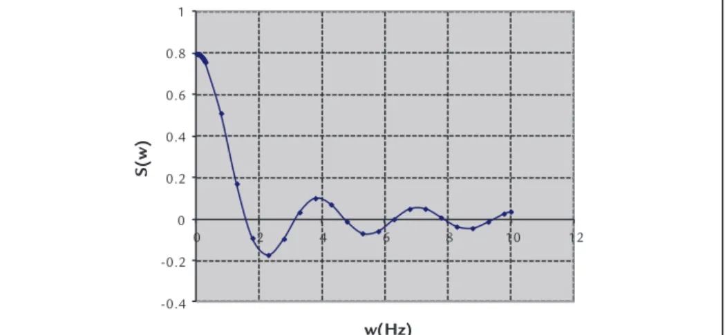
Fourier transform (Figure 5 ) of the load considered in the deterministic optimization.

-0.4 -0.2 0 0.2 0.4 0.6 0.8 1

0 2 4 6 8 10 12

S(

w

)

w(Hz)

286

The results of the optimization are tabulated in Table 2 and Figure 6.

Table 2

Results of the probabilistic optimization.

Design Variables Initial Final

1 D.V. 2 D.V. 4 D.V.

h₁(m) 1x10-2 _7.036x10-2 _1.026x10-2 _1.155x10-2

h₂(m) 1x10-2 _{-- 4.806x10}-3 _7.466x10-3

h₃(m) 1x10-2 _{-- -- 2.970x10}-3

h₄(m) 1x10-2 _{-- -- 5.776x10}-3

Obj. Func.(kg) 25.0 17.590 15.424 13.942

Const.(%) 38 44.7 44.7 44.7

Decrease Objective. Function (%) 29.64 8.76 9.6

Figure 6

Thickness Distribution throughout the plate considering 4 design variables.

7. Conclusion

A comparison of deterministic and probabilistic optimization of plate submitted to dynamic load indicates the reliability of both types of opti-mization. If there is consistency in the deinition of the deterministic and the probabilistic load, the results of both types of optimization agree quite well.

A better design in relation to the

initial design is obtained in all the analyzed cases. In Example 1, with 4 design variables, the variable least altered is variable 1 (h). This is to be expected as the elements near the point of application of the load must be more rigid. This example is illustrative, as the real plate has a constant thickness

Although the design variables

are different in the two types of op-timization, the values of the objective functions are quite similar for the cases with 2 and 4 design variables. This conclusion is to be expected as the two problems work with differ-ent design spaces and two differdiffer-ent analyses, one deterministic and the other, probabilistic.

8. References

ALVES, E. C., VAZ, L E . Optimun design of plates structures under random loadin-gs. REM-Revista Escola de Minas, v. 66, p. 41-47, 2013.

ALVES, E. C., VAZ, L. E., KATAOKA FILHO, M. Análise da sensibilidade da res-posta de estrutura submetida a carregamentos aleatório. IBERO LATIN. AMERI-CAN CONGRESS OF COMPUTATION METHODS IN ENGINEERING, 21.

Anais... Rio de Janeiro, Brazil, 2000. (Full tex in CD Rom).

FALCO, S. A. Otimização de forma de cascas submetidas a carregamento dinâmi-co. Rio de Janeiro: Pontifícia Universidade Católica do Rio de Janeiro – PUC-Rio, 2000. (Tese de Doutorado).

GOTO, S. T., NETO, E. L., KATAOKA FILHO, M. Um elemento triangular para placas e cascas laminadas. Divisão de Mecânica Espacial e Controle (DMC/ETE), Instituto Nacional de Pesquisas Espaciais – Brazil, 2000. (Proposta de Dissertação de Mestrado).

HERSKOVITS, J. Advances in structural optimization. Kluver Academic Publishers, 1995.