DETERIORATION MODELING OF STEEL MOMENT RESISTING

DETERIORATION MODELING OF STEEL MOMENT RESISTING

FRAMES USING FINITE-LENGTH PLASTIC HINGE FORCE-BASED

BEAM-COLUMN ELEMENTS

Filipe L. A. Ribeiro1

Andre R. Barbosa2

Michael H. Scott3

and Luis C. Neves4

4

Abstract

5

The use of empirically calibrated moment-rotation models that account for strength and stiffness

6

deterioration of steel frame members is paramount in evaluating the performance of steel structures prone

7

to collapse under seismic loading. These deterioration models are typically used as zero-length springs

8

in a concentrated plasticity formulation; however, a calibration procedure is required when they are used

9

to represent the moment-curvature (M₋χ)behavior in distributed plasticity formulations because the

10

resulting moment-rotation(M₋θ)response depends on the element integration method. A plastic hinge

11

integration method for using deterioration models in force-based elements is developed and validated

12

using flexural stiffness modifications parameters to recover the exact solution for linear problems while

13

ensuring objective softening response. To guarantee accurate results in both the linear and nonlinear

14

range of response, the flexural stiffness modification parameters are computed at the beginning of the

15

analysis as a function of the user-specified plastic hinge length. With this approach, moment-rotation

16

1_{Ph.D. Student, UNIC, Department of Civil Engineering, Faculdade de Ciências e Tecnologia - Universidade Nova de} Lisboa, Quinta da Torre, 2829-516 Caparica, Portugal. Visiting Ph.D. Student, School of Civil and Construction Engineering, Oregon State University, Corvallis, OR 97331-3212, USA, E-mail: f.ribeiro@fct.unl.pt

2_{Assistant Professor, School of Civil and Construction Engineering, Oregon State University, 220 Owen Hall, Corvallis,} OR 97331-3212, USA, E-mail: andre.barbosa@oregonstate.edu

3_{Associate Professor, School of Civil and Construction Engineering, Oregon State University, 220 Owen Hall, Corvallis,} OR 97331-3212, USA, E-mail: michael.scott@oregonstate.edu

models that account for strength and stiffness deterioration can be applied in conjunction with

force-17

based plastic hinge beam-column elements to support collapse prediction without increased modeling

18

complexity.

19

Keywords: Component Deterioration; Earthquake Engineering; Force-based Finite Elements; Plastic

20

Hinge Calibration; Steel

21

INTRODUCTION

22

Performance-based seismic design and assessment requires accurate nonlinear finite element models

23

that can capture the full range of structural response associated with various performance targets. In

24

the development of realistic finite element models, two main aspects need to be taken into consideration.

25

First, modes of strength and stiffness deterioration due to damage accumulation that could lead to local or

26

global collapse need to be identified. Second, the models for structural components need to be reliable,

27

robust, and computationally efficient for the entire range of the analysis. Idealized beam and column

28

models for nonlinear structural analysis vary greatly in terms of complexity and computational efficiency,

29

from phenomenological models, such as concentrated plasticity models and distributed plasticity

beam-30

column elements, to complex continuum models based on plane-stress or solid finite-elements.

31

Concentrated plasticity models (Clough et al. 1965), consist of two parallel elements, one with

32

elastic-perfectly plastic behavior to represent yielding and the other with elastic response to represent

33

post-yield hardening. Following the formal proposal by Giberson (1969), where nonlinear zero-length

34

moment rotation springs are located at both ends of a linear-elastic beam-column element, this type of

35

approach became the reference model in the development of the concentrated plasticity models. Many

36

hysteretic laws have been proposed in the last decades accounting for the most relevant phenomena

37

influencing member response up to collapse: cyclic deterioration in stiffness (Takeda et al. 1970) and

38

strength (Pincheira et al. 1999; Sivaselvan and Reinhorn 2000), pinching under load reversal (Roufaiel

39

and Meyer 1987), among many others have developed different phenomenological models that define

40

the behavior of the concentrated plastic hinges. Even though these models were developed several years

41

ago, they have been recently proposed as the main method for estimating seismic demands of frame

42

structures (Ibarra and Krawinkler 2005; Medina and Krawinkler 2005; Haselton and Deierlein 2007)

and have been presented as the preferred modeling approach in the ATC-72 guidelines (PEER/ATC

44

2010). These models allow for reliable estimation of the seismic demands in structures up to the onset

45

of collapse with limited computational cost.

46

On the opposite end of the spectrum to CPH models, continuum models are generally accepted

47

as the most reliable approach for estimating the seismic demands of structures to localized and global

48

collapse. However, these models are typically complex and require very time-consuming computations.

49

Distributed plasticity finite elements offer a compromise between concentrated plasticity models and

50

continuum finite element models.

51

Three formulations for distributed plasticity elements have been proposed in the literature:

force-52

based beam-column elements (Spacone and Filippou 1992; Neuenhofer and Filippou 1997),

displace-53

ment based column elements (Taylor 1977; Kang 1977), and the mixed formulation based

beam-54

column elements (Alemdar and White 2005). Mixed formulations typically yield the best results in

non-55

linear structural analysis, but they have not been widely adopted in the finite element software typically

56

employed in PBEE analyses.

57

Force-based beam-column elements have been shown to be advantageous over displacement-based

58

elements for material nonlinear frame analysis (Neuenhofer and Filippou 1997; Alemdar and White

59

2005; Calabrese et al. 2010) by avoiding the discretization of structural members into numerous finite

60

elements, thereby reducing the number of model degrees of freedom. In these formulations, the behavior

61

of a section is described by a fiber model or a stress resultant plasticity model (El-Tawil and Deierlein

62

1998).

63

Despite these advantages, localization issues related to non-objective strain-softening response

(Cole-64

man and Spacone 2001) led to the development of force-based finite-length plastic hinge beam-column

65

elements (FLPH elements in short) by Scott and Fenves (2006) and Addessi and Ciampi (2007).

Con-66

ceptually, these elements are composed of two discrete plastic hinges and a linear elastic region, all

67

of which are incorporated in the element integration method. Through the selection of experimentally

68

calibrated plastic hinge lengths and appropriate definition of the integration scheme, localization can be

69

avoided. The main advantages of the FLPHelements are: (i) the explicit definition of the plastic hinge

length, which allows for the recovery of meaningful local cross-section results (e.g. curvatures and

bend-71

ing moments), (ii) a clear distinction between beam-column inelasticity from the nonlinear behavior of

72

connections, and (iii) a reduced number of nodes, elements and degrees of freedom. These advantages

73

motivate the search for alternate calibration approaches as presented in this paper. Although, these

ele-74

ments have been used successfully in simulating the seismic response of structures (Berry et al. 2008),

75

they require the definition of a moment-curvature relationship and plastic hinge length to represent a

76

desired moment-rotation behavior.

77

Based on a large database of experimental results, Lignos and Krawinkler (2011) have developed and

78

validated multi-linear moment-rotation relationships that can be used to capture plastic hinge behavior

79

in simulating the deteriorating response of steel structures to collapse. Other authors have reported

sim-80

ilar moment-rotation relationships for reinforced concrete structures (Haselton and Deierlein 2007) and

81

load-displacement relationships for timber structures (Foliente 1995), which account for other modes of

82

deterioration not typically observed in steel structures. The developed moment-rotation(M₋θ)

relation-83

ships can be used directly in concentrated plastic hinge (CPH) elements following approaches presented

84

in Ibarra and Krawinkler (2005). However, several other beam-column elements formulations, such as

85

theFLPHelements, require the definition of moment-curvature relationships in the plastic hinge regions.

86

For example, for themodifiedGauss-Radau integration scheme (Scott and Fenves 2006), where the end

87

points weights are equal to the plastic hinge length Lp, moment-curvature relationships are required for

88

the two end sections. The direct scaling of the moment-rotation relationship by the plastic lengthLpin

or-89

der to obtain a moment-curvature(M₋χ)relationship (i.e. by dividing each rotation byLp(χi=θi/Lp)),

90

at first may seem a logical approach. However, this leads to erroneous results when no further calibration

91

is performed, as shown by Scott and Ryan (2013) for the common case of elasto-plastic behavior with

92

linear strain hardening under anti-symmetric bending.

93

The objective of this paper is to present a plastic-hinge calibration approach that allows for simulation

94

of structures using finite-length plastic-hinge elements that use the modified Gauss-Radau integration

95

scheme and make use of recent multi-linear moment-rotation constitutive laws that have been derived

96

from experimental results. This calibration procedure can be implemented in a finite element framework,

decreasing the user’s modeling effort, while providing accurate and reliable results.

98

The calibration procedure includes the definition of section flexural stiffness modification parameters

99

at the beginning of the nonlinear structural analysis. These modification parameters are computed as a

100

function of the plastic hinge to span length ratio by comparison of the element flexibility and the target

101

flexibility.

102

The proposed calibration methodology improves the quality and reliability of the results obtained

103

without a notable increase either in computation cost or in the complexity of structural model.

Nonethe-104

less, it is worth noting that the influence of other effects that are typically considered in 2-D frame

105

modeling of built infrastructure still need to be taken into account. Examples of relevant effects are slab

106

stiffness and strength deterioration on cyclic performance of beams, diaphragm action, load distribution,

107

and mathematical representation of damping, among others (Gupta and Krawinkler 1999). The

vali-108

dation of the calibration approach is performed for nonlinear static (pushover) analyses. However, for

109

full implementation in finite element software, nonlinear cyclic static and dynamic analyses including

110

strength and stiffness deterioration are needed in the future, as these cases fall outside the scope of this

111

paper. In addition, the proposed calibration scheme was only developed for the modifiedGauss-Radau

112

scheme, as it is found to be advantageous over other methods, namely by avoiding localization issues, in

113

the analysis of structures to seismic loading and is implemented in a finite-length plastic hinge (FLPH)

114

element (Scott and Fenves 2006). The application of the calibration approach to other integration

meth-115

ods falls outside the scope of this work.

116

PROBLEM STATEMENT

117

Empirical steel component deterioration moment-rotation behavior 118

In order to simulate component deterioration, Ibarra and Krawinkler (2005) proposed a

phenomeno-119

logical model to simulate the deterioration of steel elements, which Lignos and Krawinkler (2011)

120

adapted to define deteriorating moment-rotation relationships for plastic hinges in steel elements

us-121

ing data from a large set of experimental tests. The hysteretic behavior of the steel components is based

122

on the force-displacement envelope (backbone curve) illustrated in Figure 1. Although steel structures

123

severe ground motion, significant inelastic cyclic deformations cause deterioration of elements,

reduc-125

ing their strength and stiffness. This deterioration is significant in the analysis of steel structures under

126

cyclic lateral loads as it influences not only the resistance of the structure, but also its stiffness and its

127

resulting dynamic behavior. The backbone curve for the adopted moment-rotation model (M₋θ) is

de-128

fined in terms of: (i) yield strength and rotation (Myandθy); (ii) capping strength and associated rotation

129

for monotonic loading (Mc andθc); (iii) plastic rotation for monotonic loading (θp); (iv) post-capping

130

rotation (θpc); (v) residual strengthMr=κ×My; and (vi) ultimate rotation (θu). Other model

param-131

eters permit the definition of cyclic strength, post-capping strength, accelerated reloading stiffness and

132

unloading stiffness deterioration (Lignos and Krawinkler 2012).

133

CPHmodels 134

The empirical models described above can be used directly in the zero-length moment-rotation

135

springs of CPH elements. In the case of double curvature or anti-symmetric bending, which is the

136

reference case for the empirical moment-rotation models used in Ibarra and Krawinkler (2005) as well

137

as in Lignos and Krawinkler (2011), the global element initial flexural stiffness of the one component

138

CPH becomes 6EI/L, whereEI is the cross-section flexural stiffness andLis the element length. The

139

flexibilities of the zero-length moment-rotation springs and the element interior are additive, giving the

140

total element flexibility:

141

f=fI+fint+fJ (1)

142

where fint is the flexibility of the linear-elastic element interior andfI andfJ are the flexibilities of the

143

springs at endsIandJ, respectively.

144

The correct linear-elastic solution for the entire element is only obtained if the end rotational springs

145

are approximated as rigid-plastic. Thus, linear elastic cross-section stiffness of the springs at both ends

146

are affected by a constant n(typically greater than 1000) such that the initial stiffness of the springs is

147

large, but not so large as to pose numerical instability, as shown in Appendix I. Since the elastic stiffness

148

of the member is related to the elastic stiffness of the rotational springs and the beam-column element,

which are connected in series, the stiffness of the element interior is also affected byn, and is expressed

150

as:

151

EImod=EI

n+1

n (2)

152

which translates to spring initial stiffness given by:

153

km=n

6EImod

L , m=I,J (3)

154

Following the methodology in Ibarra and Krawinkler (2005), the ratio of post-yield to elastic stiffness

155

of the spring,α′(ratio of the tangent stiffness,kT m, to the linear elastic stiffness,km) is given by:

156

α′₌ kT m

km

= α

1+n_×(1₋α) (4)

157

where α is the nominal post-yielding to elastic stiffness ratio andα′ is assigned to the end springs in

158

theCPH model to reproduce the correct moment-rotation behavior of the member. The ratioα′is thus

159

defined such that the correct nonlinear moment-rotation stiffness of the member, defined asα_×6EI/L,

160

is recovered.

161

Finite-length plastic hinge elements 162

TheFLPHelement developed by Scott and Fenves (2006) is based on the force-based beam-column

163

finite element formulation by Spacone et al. (1996) and uses alternative numerical integration schemes

164

to account for user-defined plastic hinge lengths. The force-based beam-column finite element is

for-165

mulated assuming small displacements in a simply-supported basic system free of rigid-body

displace-166

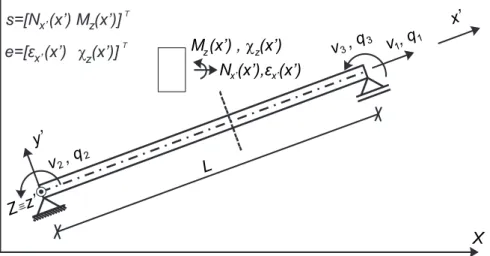
ments. Figure 2 illustrates the basic system in which the vector of element-end forces,q, the vector of

167

element deformations,v, the internal section forces,s(x), and section deformations,e(x), are shown for

168

a two-dimensional element. Section forces correspond to the axial force and bending moments, while

169

the section deformations correspond to axial strain and curvature.

Equilibrium between the section forcess(x)at a locationx, and basic element forcesqis given by:

171

s(x) =b(x)q+s0(x) (5)

172

whereb(x)is the interpolation function matrix, ands0(x)corresponds to a particular solution associated

173

with element loads. Equation 5 can be expanded into different forms depending on the number of

di-174

mensions of the problem and the beam theory selected. For the two-dimensional Euler₋Bernoulli

beam-175

column element, the basic forces areq=_{q1,q2,q3}T and the section forces ares(x) ={N(x),M(x)}T, 176

all of which are shown in Figure 2. Compatibility between element deformationsvand section

deforma-177

tionseis expressed as:

178

v=

Z L

0

b(x)Te(x)dx (6)

179

The element flexibility matrix is obtained through linearization of the element deformationsvwith

180

respect to basic forcesqand is given by:

181

f=_∂q∂v =

Z L

0

b(x)TfS(x)b(x)dx (7)

182

where fS is the section flexibility, equal to the inverse of the section stiffness fS =k−_S1. The section

183

stiffness is obtained from linearization of the constitutive relationship between section forces and section

184

deformations, kS =∂s/∂e, at the current element state. The implementation details of the force-based

185

element formulation into a displacement-based software were presented by Neuenhofer and Filippou

186

(1997) and are not reproduced here for brevity.

187

Numerical evaluation of Equation 6 is given by:

188

v=

NP

∑

bTe_|x=ξiwi (8)

189

where NP is the number of integration points over the element length, andξi andwi are the associated

locations and weights. The element flexibility is therefore given by: 191 f= NP

∑

(bTfSb|x=ξi)wi (9)

192

The main issue related to use of this formulation is the localization of strain and displacement

re-193

sponses that can be obtained in the case of strain-softening response of force-based distributed

plastic-194

ity elements (Coleman and Spacone 2001). Scott and Fenves (2006) and Addessi and Ciampi (2007)

195

proposed methods for force-based finite length plastic hinge (FLPH) integration, where the element is

196

divided in three segments, two corresponding to the plastic hinges at both ends, with lengthLpI andLpJ,

197

and a linear segment connecting both hinges (see Figure 3(a)). Thus, Equation 6 simplifies to:

198

v=

Z LpI

0

b(x)Te(x)dx+

Z L−LpJ

LpI

b(x)Te(x)dx+

Z L

L₋LpJ

b(x)Te(x)dx (10)

199

Various approaches were proposed by Scott and Fenves (2006) and Addessi and Ciampi (2007) to

200

evaluate this integral numerically; however, the focus herein is the Modified Gauss-Radau integration

201

scheme which retains the correct linear elastic solution while using the specified plastic hinge lengths as

202

the integration weights at the element ends.

203

In this method both end sections are assigned a nonlinear behavior, whereas the element interior is

204

typically assumed to have an elastic behavior, although this assumption is not necessary. The flexibility

205

of theFLPHelement can be computed as:

206

f=

Z

LpI

b(x)TfS(x)b(x)dx+

Z

Lint

b(x)TfS(x)b(x)dx+

Z

LpJ

b(x)TfS(x)b(x)dx (11)

207

whereLint is the length of the linear-elastic element interior.

208

Using themodified Gauss-Radau integration scheme for the plastic hinge regions, Equation 11 can

209

be rewritten as:

210

f=

NpI

∑

(bTfsb|x=ξi)wi+

Z

Lint

b(x)TfS(x)b(x)dx+

NpI+NpJ

∑

(bTfsb|x=ξi)wi (12)

whereNpI andNpJ are the number of integration points associated with the plastic hinges at the element

212

ends. For the modified Gauss-Radau integration NpI = NpJ =2. The element interior term can be

213

computed exactly when the element interior is elastic and there are no member loads. Nonetheless, the

214

element interior can also be analyzed numerically. In this case, the Gauss-Legendre integration scheme

215

is appropriate to integrate the element interior. If two integration points are placed in this region, a total

216

of six integration points are defined along the element length. The location ξi of the integration points

217

associated with themodifiedGauss-Radau plastic hinge integration, represented in Figure 3(a), are given

218

by:

219

ξ=_{ξI,ξint,ξJ} (13)

220

where:

221

ξI=

n

0;8L₃pI

o

ξint=

n

4Lp+L₂int ×

1₋√1

3

; 4Lp+L₂int ×

1+√1

3 o

ξJ=

n

L₋8LpJ

3 ;L o

(14)

222

The corresponding weightswiare given by:

223

w=_{wI,wint,wJ} (15)

224

where:

225

wI=

LpI; 3LpI

wint=

n Lint 2 ; Lint 2 o

wJ=

3LpJ;LpJ

(16)

226

In this case, the element flexibility is then given by:

227

f=

6

∑

(bTfsb|x=ξi)wi (17)

228

where this equation is consistent with points and weights shown in Figure 3(a).

CALIBRATION OF FORCE-BASED FINITE-LENGTH PLASTIC HINGE ELEMENTS

230

TheFLPHformulation requires the definition of moment-curvature relationships in the plastic hinge

231

region, and subsequent procedures to relate these relationships to the moment-rotation response of the

232

element. In this section, a novel method for calibration of the moment-rotation behavior of finite-length

233

plastic hinge force-based frame elements is proposed for arbitrary plastic hinge lengths. With this

ap-234

proach, moment-rotation models that account for strength and stiffness deterioration can be applied in

235

conjunction with FLPH models to support collapse prediction of frame structures. The approach

in-236

cludes an automatic calibration procedure embedded in the numerical integration of the element, freeing

237

the analyst of this task. The calibration procedure is formulated for themodifiedGauss-Radau integration

238

scheme. However, it can be applied to other plastic hinge methods proposed by Scott and Fenves (2006)

239

and Addessi and Ciampi (2007), function of the weight and location of the integration points used in the

240

calibration.

241

Calibration Procedure 242

The main goals of this procedure are to:

243

1. Use empirical moment-rotation relationships that account for strength and stiffness deterioration

244

to model the flexural behavior of the plastic hinge region;

245

2. Guarantee that the flexural stiffness is recovered for the nominal prismatic element during the

246

entire analysis; and

247

3. Allow the definition of arbitrary plastic hinge lengths by the analyst.

248

The presented calibration procedure is performed at the element level through the introduction of

249

section flexural stiffness modification parameters at internal sections of the beam-column element

mak-250

ing it possible to scale a moment-rotation relation in order to obtain moment-curvature relations for the

251

plastic hinge regions. Defining the moment-rotation stiffness of the plastic hinge regions as:

252

kM−θ= α

6EI

L (18)

and making use of a user-defined plastic hinge length at either end of the element (LpI andLpJfor ends

254

I andJ, respectively), the moment-curvature relations can be defined as:

255

kM−χ= α

6EI

L ×LP{I,J} (19)

256

As highlighted by Scott and Ryan (2013), the moment-rotation and moment-curvature relations are

iden-257

tical for L_P{I,J}/L=1/6. However, for any other plastic hinge length, the definition of the

moment-258

curvature via direct scaling of the moment-rotation given by Equation 19 yields incorrect section

stiff-259

ness, which in turn lead to incorrect member stiffness. The calibration procedure presented herein

com-260

pensates for the incorrect stiffness of the plastic hinge moment-curvature relationship by modifying the

261

flexural stiffness of each of the four internal sections (integration pointsξ2,ξ3,ξ4andξ5in Figure 3(a)), 262

assumed to remain linear elastic throughout the analysis, using one of three different parameters,β1,β2,

263

andβ3, shown in Figure 3(b).

264

Theβmodification parameters are quantified such that the element flexibility matrix is: (i) within the

265

elastic region, equal to the analytical solution for an elastic prismatic element; (ii) after yielding, identical

266

to the target flexibility, i.e. is similar to the user-definedM₋θbehavior. The target flexibility matrix in

267

the elastic and nonlinear regions can be provided by theCPH model using Equations 1 to 4. Then, the

268

modification parameters are defined based on the equivalence of the flexibility matrices associated with

269

the CPH andFLPH models. The target flexibility can be computed using different models and herein

270

the models defined by Lignos and Krawinkler (2011) are used in the derivations. In the calibration

271

procedure, double curvature or anti-symmetric bending is assumed to obtain the elastic stiffness of the

272

structural element. This is a common result of the lateral loading and boundary conditions considered in

273

seismic analysis of frame structures. In this case, the elastic elementM₋θstiffness is 6EI/L. However,

274

the calibration procedure shown herein is valid for any element moment-rotation stiffness and moment

275

gradient.

Derivation of Modification Parameters 277

For the 2D beam-column element, a system of three integral equations corresponding to each of

278

the unique flexural coefficients of the element flexibility matrix is constructed. The flexibility matrix

279

coefficients obtained from Equation 17, corresponding to theFLPH, are equated to the flexibility matrix

280

coefficients obtained from Equation 1, associated with aCPHmodel and the empirical model. From this

281

system of equations, the three elastic stiffness modification parameters,β1,β2, andβ3, can be computed

282

as a function ofLpI,LpJ,Landn, which is the elastic stiffness modification parameter of theCPHmodel.

283

The code for solving the system of equations, which is implemented in thewxMaximasoftware (Souza

284

et al. 2003) and is presented in the Appendix II. Whenntends to infinity,β1,β2andβ3are given by:

285

β1 = −

54LpIL3−6LpI(60LpI+60LpJ)L2+6LpI(96L2pI+288LpILpJ+96L2pJ)L−6LpI(256L2pILpJ+256LpIL2pJ)

L(3L₋16LpJ)(L2−20LLpI+4LpJL+64L2pI)

286

β2 = −

3(4LpI−L+4LpJ)(3L2−12LLpI−12LLpJ+32LpILpJ)

L(3L₋16LpI)(3L−16LpJ)

(20)

287

β3 = −

54LpJL3−6LpJ(60LpI+60LpJ)L2+6LpJ(96L2pI+288LpILpJ+96L2pJ)L−6LpJ(256L2pILpJ+256LpIL2pJ)

L(3L₋16LpI)(L2−20LLpJ+4LpIL+64L2pJ)

288

289

If both plastic hinges have the same length, i.e. Lp=LpI =LpJ, Equation 20 simplifies significantly

290

to:

291

β1 = β3=−

6 3L2Lp−24L L2p+32L3p

L(L₋8Lp)2

292

β2 =

3 3L3₋48L2Lp+224L L2p−256L3p

L(3L₋16Lp)2

(21)

293

It is worth noting that in Equation 21 there are singularities inβ1andβ3 forLp/L=1/8 and in β2

294

forLp/L=3/16, which correspond to cases in which: (i) the length of the elastic element interior,Lint,

295

is equal to zero and (ii) the two internal integration pointsξ2andξ5shown in Figure 3(b) are co-located.

296

In Figure 4 the flexural stiffness modification parameters of Equation 21 are represented as a function

297

both plastic hinges have the same flexural stiffnessα16EILp/L=α26EILp/L. Note that the calibration 299

procedure is valid whenLint <0, i.e.Lp/L>1/8.

300

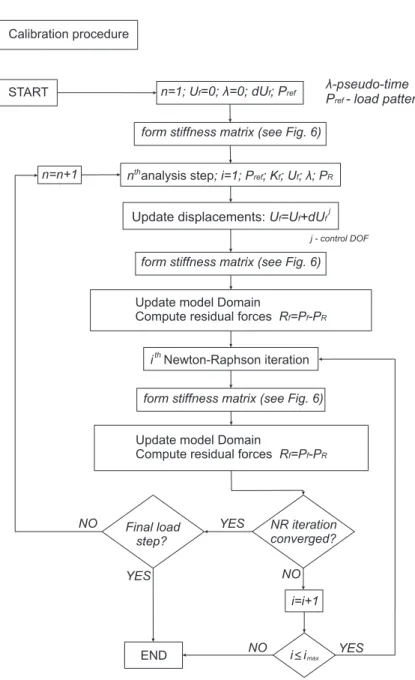
The proposed calibration procedure is illustrated in Figure 5 for the specific case of a nonlinear static

301

(pushover) analysis. The pushover analysis is conducted by controlling a jth degree of freedom (DOF).

302

Furthermore, the displacementUf and pseudo-time λ are initialized to zero, and the displacement

in-303

crement dUf for the control DOF and the reference load patternPre f are also initialized. The stiffness

304

matrix Kf is computed in the form stiffness matrix procedure (see Figure 6) at the beginning of each

305

analysis step and each NR iteration. In this procedure, the parameters α1 and α2 are calculated based

306

on the committed (converged in a previous step) element forces and deformations, as well as the

tan-307

gent stiffness. In the first analysis step, the section stiffness modification parameters β1, β2 andβ3 are

308

computed, as shown in Figure 6. Once the stiffness modification parameters are computed, the stiffness

309

matrix is computed through inversion of the flexibility matrix. The stiffness matrix is obtained

consid-310

ering the integration points (IPs) of themodifiedGauss-Radau integration scheme shown in Figure 3(b).

311

Transformation from the basic to the local coordinate system is performed with the matrixAf. From this

312

point onward a traditional NR algorithm is used, repeating the above procedure at the beginning of each

313

analysis step and at each NR iteration. Different strategies can be used in updating the model state

deter-314

mination, namely: (i) update state of the model domain (displacements, pseudo-time, forces) using the

315

residual tangent displacement from the previous iteration; (ii) decrease the displacement increment and

316

update the model domain trying to overcome convergence problems; (iii) change the numerical method

317

used (either for this analysis step only or for all remaining steps); and (iv) change the tolerance criteria

318

(if that is admissible for the case being analyzed). In case the NR method is not able to converge after a

319

user-defined maximum number of iterations, imax, the analysis is stopped, and is considered not to have

320

converged. Illustrative examples are presented in the following sections. Different solution algorithms

321

may be used to solve the nonlinear residual equations (De Borst et al. 2012; Scott and Fenves 2010).

322

The Newton-Raphson (NR) algorithm is one of the most widely used and is a robust method for solving

323

nonlinear algebraic equations of equilibrium. In this figure (Figure 5) the flowchart for the calibration

324

procedure is exemplified using the NR algorithm.

NUMERICAL EXAMPLES

326

The proposed methodology was applied to a set of simply supported beams subjected to end moments

327

and considering different plastic hinge lengths, as well as a simple steel frame structure. The beams are

328

analyzed considering a pushover analysis, where rotations are incremented until reaching an ultimate

329

rotation. For the first beam, equal moments are applied at each support, while in the second case, the

330

moment applied at the left support is half of that applied to the right support. The steel element properties,

331

including the parameters considered for the deterioration model, are presented in Table 1.

332

Example 1 333

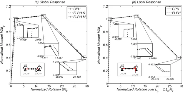
A simply supported beam is analyzed considering equal moments and rotations applied at both ends.

334

Figure 7(a) shows the element end moment plotted against the element end rotation. A local response,

335

corresponding to the rotation of a section at a distanceLpfrom the support is also plotted against the end

336

moment in Figure 7(b). The rotation at a distanceLpfrom the support, in theCPH model, must consider

337

the rotation of the zero-length spring and the deformation of the elastic segment of lengthLp.

338

In this figure, the plastic rotation of theCPH model is computed obtained by adding the rotation of

339

the zero-length spring to the rotation of the elastic element over a length ofLp. The former is obtained

340

by multiplying the curvature (χ) of the end section of the element byLp.

341

TheCPHcurve denotes the results obtained using a concentrated plastic hinge model, following the

342

procedure employed by Lignos and Krawinkler (2012), and serves as a benchmark. Figure 7(a) shows

343

that end rotations obtained using the CPH model present an initial linear elastic response up to the

344

yielding point, defined by the yielding moment-rotation pairMy,CPH−θy,CPH. Then, a linear hardening

345

region connects the yielding point to the capping point (Mc,CPH−θc,CPH) and a linear softening region

346

links the capping point to the residual moment-rotation point (Mr,CPH−θr,CPH), which is followed by

347

a plastic region that extends to θU. The second model considered (FLPH S) corresponds to the use of

348

finite length plastic hinge elements, defining the moment-curvature relation through direct scaling of the

349

rotation parameters (θy,θc,θpc,θr, andθu) by the plastic hinge lengthLpand no further calibration. The

350

results show that this approach leads to erroneous results, as the elastic stiffness obtained is significantly

351

lower than the target, and higher rotations are obtained in the softening branch. If the moment curvature

is calibrated (curveFLPH M) using the proposed method, it is possible to reproduce theCPH behavior

353

of the beam exactly for the entire analysis. Although the global response is in perfect agreement, Figure

354

7(b) shows that the local response is different when the CPHor theFLPH M models are used. For the

355

FLPH models, local response in Figure 7(b) corresponds to the integration of the end section curvature

356

(χ) over the plastic hinge length Lp (χ×Lp). This result is equal for the FLPH S and the FLPH M

357

models since the end sections of both models are defined in a similar manner (only the interior sections

358

are affected by the flexural modification parameters).

359

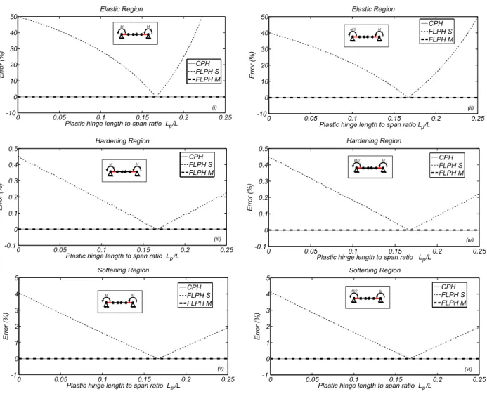
Figure 9(a) shows the errors associated with the different models and different plastic hinge lengths.

360

The errors are defined as the ratio between the computed slopes of the elastic, hardening, and softening

361

branches, and the respective target moment-rotation defined in Lignos and Krawinkler (2011). The

362

results show that: (i) the FLPH M calibration procedure provides accurate results when compared to

363

the results obtained using CPH for the elastic, hardening and softening ranges of the response; (ii) the

364

FLPH Sprocedure, where a scaled moment-curvature relation is used without further calibration, results

365

in significant errors. It is worth noting that only for Lp/L=1/6 does the FLPH S model result in the

366

exact moment-rotation at yielding and at the capping point, as previously shown by Scott and Ryan

367

(2013). The results from this example highlight the the advantages of the calibration procedure proposed

368

herein, namely showing that accurate results can be achieved for varying lengths of the plastic hinge and

369

for cases considering softening.

370

Example 2 371

To show calibration for other moment gradients in the beam element, an identical beam to that from

372

the previous example is analyzed considering the left moment equal to half of the right moment. As a

373

result the left end of the beam is always in the elastic range, and the beam does not deform in double

374

curvature. However, as shown in Figure 8, the results obtained for a plastic hinge lengthLp/L=1/16 are

375

consistent with those obtained in Example 1. In fact, the results obtained with the scaled moment

cur-376

vature relation without calibration (FLPH S) show significant errors from the elastic range, propagating

377

over the entire range of analysis. When calibration is considered (FLPH M) the results are corrected and

378

perfect agreement is found betweenCPH andFLPH M models. Figure 9(b) shows the results obtained

considering several plastic hinge lengths. The errors are computed by comparing the slopes of the elastic,

380

hardening and softening branches of the twoFLPHelements with theCPHmodel. Results show that the

381

analysis presented forLp/L=1/16 is valid for all values of the plastic hinge length. Furthermore, the

382

results show that the proposed calibration procedure is applicable to different moment gradients besides

383

anti-symmetric bending.

384

Frame structure 385

A single-bay three-story frame with uniform stiffness and strength over its height (see Figure 10) is

386

used to illustrate the application of the calibration procedure described above. A dead load of 889.6kN is

387

applied to each story, giving a total structure weightW of 2669kN. The flexural stiffnessEI is identical

388

for beams and columns with values given in Table 1. Plastic hinges form at beam ends and at base

389

columns. The other columns are assumed to remain elastic. Pushover analyses of the frame are conducted

390

in the OpenSees framework (McKenna et al. 2000) using a P-Delta geometric transformation for the

391

columns. Results obtained with modelFLPH Mare compared to results obtained using theCPHmodels.

392

It is worth noting that in steel W-shape beams with shape factors (k=Mp/My) of approximately 1.12,

393

the plastic hinge length is taken as 10% of the distance between the point of maximum moment and the

394

inflection point (Bruneau et al. 1998). This value is slightly larger, approximately 12.5%, at the center

395

of beams that are subjected to distributed loads. Thus, for members in a state of anti-symmetric double

396

curvature, it is suggested that a plastic hinge length betweenL/20 andL/16 be used.

397

Figure 11(a) shows the normalized base shear (V/W) versus roof drift ratio for the three models and

398

Figure 11(b) illustrates the beam moment-rotation response. The results obtained for this frame show

399

that the conclusions drawn for the two previous examples hold, namelyFLPH Sshould not be used as a

400

procedure for converting from empirical moment-rotation relations to moment-curvature relations when

401

FLPH elements are used, andFLPH M is an adequate procedure that produces objective results without

402

computationally expensive iterative/updating procedures.

403

CONCLUSIONS

404

The present work proposes a calibration procedure that allows the use of finite-length plastic hinge

405

at the section and element levels. The use of scaled but uncalibrated moment-curvature relationships in

407

FLPHelements leads to significant errors in both local and global responses and is therefore not adequate

408

for structural analysis. The new calibration procedure is performed at the element level through the

in-409

troduction of section flexural stiffness modification parameters (β), which are computed at the beginning

410

of the analysis as a function of the user defined plastic hinge lengths. The modification parameters are

411

obtained by equating element flexural coefficients of the flexibility matrix and target flexibility matrix,

412

where the latter is given by the user-defined moment-rotation relation and is computed in this work using

413

aCPHmodel. Nonlinear static analyses of two simply supported beams and pushover analysis of a steel

414

moment-resisting frame were performed considering different plastic hinge lengths. The results

illus-415

trate that the exact linear elastic stiffness can be recovered for linear problems while ensuring objective

416

response after the onset of deterioration. The cases studied as well as error analysis based on

analyti-417

cal expressions show that the calibration procedure is valid for any moment gradient. Even though the

418

proposed calibration procedure has only been validated for multi-linear moment-rotation relationships,

419

it is, in principle, possible to use it with other constitutive laws, where moment-rotation can be related to

420

moment-curvature by a user-defined plastic hinge length. The calibration procedure was validated at the

421

section level for bending moments and rotations only, but similar approaches may be used for cases in

422

which the interaction between bending and axial deformations is considered. The accuracy and stability

423

of the proposed calibration procedure remains to be studied for nonlinear dynamic time-history analysis

424

of steel moment frame buildings.

ACKNOWLEDGEMENTS

426

In the development of this research work, the first and fourth authors would like to acknowledge the

427

support of the Portuguese Science and Technology Foundation through the program SFRH/BD/77722/2011

428

and UNIC Research Center at the Universidade Nova de Lisboa. The support of the School of Civil and

429

Construction Engineering at Oregon State University to the second and third authors is gratefully

ac-430

knowledged. The opinions and conclusions presented in this paper are those of the authors and do not

431

necessarily reflect the views of the sponsoring organizations.

432

References

433

Addessi, D. and Ciampi, V. (2007). “A regularized force-based beam element with a damage plastic

434

section constitutive law.”International Journal for Numerical Methods in Engineering, 70(5), 610–

435

629.

436

Alemdar, B. and White, D. (2005). “Displacement, flexibility, and mixed beam–column finite element

437

formulations for distributed plasticity analysis.” Journal of structural engineering, 131(12), 1811–

438

1819.

439

Berry, M., Lehman, D., and Lowes, L. (2008). “Lumped-plasticity models for performance simulation

440

of bridge columns.”ACI Structural Journal, 105(3).

441

Bruneau, F., Uang, C-M. and Whittaker, A. (1998). “Ductile design of steel structures.”, New York:

442

McGraw-Hill, 1998.

443

Calabrese, A., Almeida, J., and Pinho, R. (2010). “Numerical issues in distributed inelasticity modeling

444

of rc frame elements for seismic analysis.”Journal of Earthquake Engineering, 14(S1), 38–68.

445

Clough, R., Benuska, K., and Wilson, E. (1965). “Inelastic earthquake response of tall buildings.”Third

446

World Conference on Earthquake Engineering, Wellington, New Zealand.

447

Coleman, J. and Spacone, E. (2001). “Localization issues in force-based frame elements.”ASCE Journal

448

of Structural Engineering, 127(11), 1257–1265.

449

Cook, R. D., Malkus, D. S., Plesha, M. E., and Witt, R. J. (2001). Concepts and Applications of Finite

450

Element Analysis. Wiley; 4 edition.

De Borst, R., Crisfield, M., Remmers, J., and Verhoosel, C. (2012).Nonlinear finite element analysis of 452

solids and structures. John Wiley & Sons.

453

El-Tawil, S. and Deierlein, G. G. (1998). “Stress-resultant plasticity for frame structures.” Journal of

454

Engineering Mechanics, 124(12), 1360–1370.

455

Foliente, G. (1995). “Hysteresis modeling of wood joints and structural systems.” ASCE Journal of

456

Structural Engineering, 121(6), 1013–1022.

457

Giberson, M. (1969). “Two nonlinear beams with definitions of ductility.” Journal of the Structural

458

Division, 95(2), 137–157.

459

Gupta, A. and Krawinkler, H. (1999). “Seismic demands for performance evaluation of steel moment

460

resisting frame structures.”Report No. 132, The John A. Blume Earthquake Engineering Center.

461

Haselton, C. and Deierlein, G. (2007). “Assessing seismic collapse safety of modern reinforced

con-462

crete frame buildings.”Report No. 156, The John A. Blume Earthquake Engineering Center, Stanford

463

University.

464

Ibarra, L. F. and Krawinkler, H. (2005). “Global collapse of frame structures under seismic excitations.”

465

Report No. 152, The John A. Blume Earthquake Engineering Research Center, Department of Civil

466

Engineering, Stanford University, Stanford, CA.

467

Kang, Y. (1977). Nonlinear geometric, material and time dependent analysis of reinforced and

pre-468

stressed concrete frames. UC-SESM Report No. 77-1, University of California, Berkeley.

469

Lignos, D. and Krawinkler, H. (2012). “Development and utilization of structural component

470

databases for performance-based earthquake engineering.”ASCE Journal of Structural Engineering,

471

doi:10.1061/(ASCE)ST.1943-541X.0000646.

472

Lignos, D. G. and Krawinkler, H. (2011). “Deterioration modeling of steel components in support of

473

collapse prediction of steel moment frames under earthquake loading.” ASCE Journal of Structural

474

Engineering, 137(11), 1291–1302.

475

McKenna, F., Fenves, G., and Scott, M. (2000). Open system for earthquake engineering simulation.

476

University of California, Berkeley, CA.

477

Medina, R. and Krawinkler, H. (2005). “Evaluation of drift demands for the seismic performance

ment of frames.”ASCE Journal of Structural Engineering, 131(7), 1003–1013.

479

Neuenhofer, A. and Filippou, F. (1997). “Evaluation of nonlinear frame finite-element models.”Journal

480

of Structural Engineering, 123(7), 958–966.

481

PEER/ATC (2010). “Modeling and acceptance criteria for seismic design and analysis of tall buildings.”

482

Report No. 72-1, ATC - Applied Techonology Council.

483

Pincheira, J., Dotiwala, F., and D’Souza, J. (1999). “Seismic analysis of older reinforced concrete

484

columns.”Earthquake Spectra, 15(2), 245–272.

485

Roufaiel, M. and Meyer, C. (1987). “Analytical modeling of hysteretic behavior of r/c frames.” ASCE

486

Journal of Structural Engineering, 113(3), 429–444.

487

Scott, M. H. and Fenves, G. L. (2006). “Plastic hinge integration methods for force-based beam-column

488

elements.”ASCE Journal of Structural Engineering, 132(2), 244–252.

489

Scott, M. H. and Fenves, G. L. (2010). “Krylov subspace accelerated newton algorithm: Application to

490

dynamic progressive collapse simulation of frames.”ASCE Journal of Structural Engineering, 136(5),

491

473–480.

492

Scott, M. H. and Ryan, K. L. (2013). “Moment-rotation behavior of force-based plastic hinge elements.”

493

Earthquake Spectra, 29(2), 597–607.

494

Sivaselvan, M. and Reinhorn, A. (2000). “Hysteretic models for deteriorating inelastic structures.”ASCE

495

Journal of Engineering Mechanics, 126(6), 633–640.

496

Souza, P. N., Fateman, R., Moses, J., and Yapp, C. (2003). The Maxima book.

497

http://maxima.sourceforge.net.

498

Spacone, E. and Filippou, F. (1992).A Beam Model for Damage Analysis of Reinforced Concrete

Struc-499

tures Under Seismic Loads. Department of Civil Engineering, University of California.

500

Spacone, E., Filippou, F., and Taucer, F. (1996). “Fibre beam-column model for non-linear analysis of

501

R/C frames: Part I. formulation.”Earthquake Engineering and Structural Dynamics, 25(7), 711–726.

502

Takeda, T., Sozen, M., and Nielson, N. (1970). “Reinforced concrete response to simulated earthquakes.”

503

ASCE Journal of the Structural Division, 96(12), 2557–2573.

504

Taylor, R. (1977). “The nonlinear seismic response of tall shear wall structures.” Ph.D. thesis,

ment of Civil Engineering, University of Canterbury, 207pp.

506

Zareian, F. and Medina, R. A. (2010). “A practical method for proper modeling of structural damping in

507

inelastic plane structural systems.”Computers & Structures, 88(1-2), 45–53.

Appendix I. ERROR IN THE MODEL ELASTIC STIFFNESS ASSOCIATED WITH THE CPH SPRINGS

509

ELASTIC STIFFNESS AMPLIFICATION FACTOR

510

InCPH models, the elastic stiffness amplification factor (n) should be chosen carefully as an

exces-511

sively large value would pose numerical problems, while a value that is not sufficiently large will lead to

512

erroneous results in the elastic range. In this Appendix, elastic stiffness errors associated with values of

513

n<1000 are computed.

514

Considering that each member can be represented by two end rotational springs and an elastic frame

515

element in series, the flexibilities of the springs and the frame element in aCPH element are additive.

516

Using the tangent stiffnesses,kT IandkT J, of each rotational spring, the member flexibility is:

517

fb=



 

1/kT I 0

0 0



 +

L

6EI×



 

2 ₋1

−1 2

  +    0 0

0 1/kT J





 (A.1)

518

To recover the correct linear-elastic solution for the entire CPH model, the end rotational springs

519

need to be approximated as rigid-plastic with an initial stiffness that is large, but not so large to pose

520

numerical instability. This is akin to the selection of large penalty values when enforcing multi-point

521

constraints in a structural model (Cook et al. 2001). The ratio of flexibility coefficient fb(1,1)to the

522

exact linear-elastic solution L/(3EI) is plotted in Figure 12 versus the elastic stiffness amplification

523

factor, which scales the characteristic element stiffnessEI/L(kI =n×EI/L).

524

As shown in Figure 12, the ratio between the elastic stiffness recovered using differentnvalues for

525

theCPH model and the target elastic stiffness (L/3EI) varies from 1.30 (30% error) forn=10 to 1.003

526

(0.3% error) forn=1000. Thus, to recover the elastic solution with negligible errors, it is suggested that

527

a value ofn=1000 be used.

528

Although the suggested value of n_≥1000 allows for recovery of the elastic stiffness, several

au-529

thors have highlighted that there is an increased likelihood of non-convergence of nonlinear time-history

530

response analyses if such a large value of n is used. For this reason, Zareian and Medina (2010) have

531

suggested the use of n=10. However, the use of such a low value ofncan lead to overestimating the

532

elastic flexibility of the elements up to 30%, which could lead to approximately 13% error in natural

frequencies of vibration.

Appendix II. COMPUTATION OF THE SECTION FLEXURAL STIFFNESS MODIFICATION

535

PARAMETERS

536

.

537

The following code was implemented in thewxMaximasoftware (Souza et al. 2003).

538

• Unknowns

539

β1,β2,β3 (A.2)

540

• Input data

541

y : [0,8/3_×LpI,L−8/3×LpJ,L];

542

w : [LpI,3_×LpI,3×LpJ,LpJ]; (A.3)

543

mp : [α1×6×LpI/L,β1,β3,α2×6×LpJ/L]; 544

• Computation of the element flexibility matrix (flexural terms only)

545

f1:matrix([0,0],[0,0]); (A.4) 546

• Plastic hinges integration points

547

for i : 1 to 4 do

548

(f1 : f1+transpose(matrix([0,0],[y[i]/L−1,y[i]/L])). (A.5) 549

matrix([0,0],[y[i]/L₋1,y[i]/L])_×w[i])_×

550

(1/(mp[i]_∗EI));

551

• Interior region

552

f1 : f1+integrate(transpose(matrix([0,0],[x/L−1,x/L])). 553

matrix([0,0],[x/L₋1,x/L])_×(1/(β2×EI)), (A.6) 554

x,4_×LpI,L−4×LpJ);

555

• Computation of the target flexibility matrix using aCPHmodel (flexural terms only)

556

• CPHmodel parameters

557

EImod : EI×(n+1)/n;

558

Kspring : n×6×EImod/L; (A.7)

559

• Model flexibility matrix

561

f2 : matrix([1/(mp2[1]×kspring),0],[0,1/(mp2[2]×kspring)]);

562

f2 : f2+integrate(transpose(matrix([0,0],[x/L−1,x/L])). (A.8) 563

matrix([0,0],[x/L₋1,x/L])_×(1/(EImod)),

564

x,0,L);

565

• Solve the system of equations for obtaining unknowns

566

eq1 : f1[1,1] = f2[1,1]; 567

eq2 : f1[1,2] = f2[1,2]; 568

eq3 : f1[2,2] = f2[2,2]; (A.9)

569

sol : solve([eq1,eq2,eq3],[β1,β2,β3]); 570

• Although the previous step already gives a solution for the problem, it is useful to obtain the

571

solution without dependency onn. Thus, the solution,sol, is evaluated whenntends to infinity

572

limit(sol,n,in f); (A.10)

List of Tables

574

1 Element properties for numerical examples . . . 28

Table 1. Element properties for numerical examples

Geometric parameters Moment-rotation model parameters

Inertia (m4) Area (m2) My(kNm) Mc/My θp(rad) θpc(rad)

Example 1 and 2 0.0002 0.0073 320.78 1.05 0.0692 0.168

Frame Beams 0.0111 0.0551 1911.0 1.05 0.025 0.25

List of Figures

576

1 Adapted modified Ibarra-Krawinkler model: (a) backbone curve; and (b) basic modes of

577

cyclic deterioration . . . 30

578

2 Basic system for two-dimensional frame elements . . . 31

579

3 Modified Gauss-Radau integration scheme . . . 32

580

4 Flexural stiffness modification parametersβ1,β2andβ3as a function of the plastic hinge

581

length to span ratioLp/L . . . 33

582

5 Calibration procedure for a nonlinear static structural (pushover) analysis . . . 34

583

6 Flowchart for computation of element stiffness matrix . . . 35

584

7 Example 1 - basic system with equal moments at both ends and plastic hinge length

585

Lp/L=1/16 . . . 36

586

8 Example 2 - basic system with different moments at both ends and plastic hinge length

587

Lp/L=1/16 . . . 37

588

9 Errors in the slopes of the elastic, hardening and softening regions for theCPH,FLPH S

589

andFLPH Mmodels during a monotonic analysis . . . 38

590

10 Steel moment frame . . . 39

591

11 Example three-story frame used to demonstrate the proposed calibration procedures . . . 40

592

12 Computed elastic flexibility coefficient of concentrated plasticity model versus

rigid-593

plastic approximation of end springs . . . 41

M o m e n t M

Chord rotation ?

Initial backbone curve

Ke

M

M

?

?

?

?

M

=?M

?

?

c

(a)

Moment M

θ θ

θ

θ

θ

θ

θ

u r c

y

p pC

e

y r

y c

k

Y

X

y’

x’ v , q1 1

v , q2 2

v , q3 3

L

Z z’

M (x’) ,_z c_z( )x’ N (x’), (x’)_x’ ε_x’

s=[N (x’) M (x’)]_{x’ z}

e=[ε_x’(x’) c_z(x’)] T

T

(a) Modified Gauss-Radau Integration

Linear Elastic

x1 x2 x6

S 1 k = S 6 k = S 2

k = S

0 0 5 EA k EI = pI L pI

8L /3

pJ

L

pJ 3_L

=0 =

pI 3_L

x5=L- L /8pJ3 =L

0

0 EA

EI ( )c₆

0

0 EA

EI ( )c₁

0 0 EA EI S 0 0 4 EA k EI =

x4=4L +L / ( + / )p int2 1 1 3

S 0 0 3 EA k EI =

x₃=4L +L / ( - / )p int 2 1 1 3

int

L

(b) Integration with Section Modification Parameters

x1 x2 x6

S 1 0 0 1 pI EA k L 6EI L a = S 2 0 0 6 pJ EA k L 6EI L a = S 1 0 0 2 EA k EI b = S 3 0 0 5 EA k EI b = pI

L 3LpI 3LpJ LpJ

x5 Linear Elastic S 0 0 4 EA k EI = x₄ S 0 0 3 EA k EI = x3 int L 2 b 2 b

0 0.05 0.1 0.15 0.2 0.25 -20

-15 -10 -5 0 5 10 15 20

Plastic hinge to span length ratio L_p/L

Flexural stiffness

modification parameters

β

β

1

β

2

β

3 L_p/L = 1/20

β₁= -1.567

β 2= 0.699 β₃= -1.567

Lp/L = 1/10 β

1= -13.80 β

2= 0.282 β

3= -13.80

Lp/L = 1/16 β

1= -2.438 β₂= 0.609

β 3= -2.438

L_p/L = 1/6

β 1= 1.0 β

2= 1.0 β

3= 1.0

Lp

/L=1/8

Lp

/L=3/16

Lp

/L=1/6

START n=1; Uf=0; =0; dU ; Pλ f ref

Calibration procedure

form stiffness matrix (see Fig. 6)

nthanalysis step; i=1; P ; K ; U ; ; Pref f f λ R

f f f

Update displacements:U =U +dU

form stiffness matrix (see Fig. 6)

λ-pseudo-time P - load patternref

j - control DOF

ithNewton-Raphson iteration

form stiffness matrix (see Fig. 6)

NR iteration converged? Final load

step?

END

j

i=i+1 n=n+1

YES

YES NO

NO

Update Domain

Compute residual forces model

R =P -Pf f R

Update Domain

Compute residual forces model

R =P -Pf f R

YES i i≤max

NO

START

Sectional constitutive relation. For the end IPS ( , ) computeξ ξ1 6 α1andα2 c

α1=k ( ) /s 1n k ( )sc10 α2=k ( ) /sc6n k ( )sc60

Update basic displacements:U =A xUb f f

Computeβ β1, 2andβ3upon

evaluation ofLpandL

Form Stiffness Matrix Procedure

Compute flexibility matrix for all IPs

Compute element flexibility matrix:

where:

1,2

0 0 1/EA

6EI

a

fs =|x=ξ1,6

1,3

0

0 1/EA

EI)

β

fs =|x=ξ2,5

2

0

0 1/EA

EI) 1/(β

Compute stiffness matrix at basic level:k =fb -1

Compute stiffness matrix at local level:K =A .k .Af Tf b f

Compute vector of resisting forcesPR END

A local to basic transformation matrix

f

-LpI,J

L

1/( ) 1/(

n=1? YES

NO

å =

= =

6

1

i

i x i s T_{f b w} b f

i) |

( , x

fs =|x=ξ3,4

Figure 7. Example 1 - basic system with equal moments at both ends and plastic hinge length

M M/2

θ

L =L/16p L =L/16p

1.2 1.2

M M/2

c

L =L/16p L =L/16p

c

Figure 8. Example 2 - basic system with different moments at both ends and plastic hinge length