Brazilian Microwave and Optoelectronics Society-SBMO received 05 Apr 2017; for review 06 Apr 2017; accepted 21 Sep 2017
Abstract— In this paper, an improved neural networks (INN)
strategy is proposed to design two waveguide filters(Pseudo-elliptic waveguide filter and Broad-band e-plane filters with improved stop-band). INN is trained by an efficient optimization algorithm called teaching–learning-based optimization (TLBO). To validate the effective of this proposed strategy, we compared the results of convergence and modeling obtained with a population based algorithm that is widely used in training NN namely Particle Swarm Optimization (PSO-NN). The results show that the proposed INN has given better results.
Index Terms— Improved neural networks, modeling, teaching–
learning-based optimization, waveguide filters.
I. INTRODUCTION
The full wave EM solvers [1] have been used to design the microwave filter for a long time. With
the increasing complexity of wireless and satellite communication hardware, the use of EM solver
takes a considerable amount of time. Recently, artificial neural network (ANN) has been proven to be
a fast and effective means of modeling complex electromagnetic devices. It has been recognized as a
powerful tool for predicting device behavior for which no mathematical model is available or the
device has not been analyzed properly yet. ANN can be trained to capture arbitrary input-output
relationship to any degree of accuracy. Once a model is developed it can be used over and over again.
The trained model delivers the output parameters very quickly. For these attractive qualities, ANN has
been applied to different areas of engineering’s [2] - [4].
Training of neural networks (NN) is an important step; it is based on optimization of
weights of NN to minimize the mean square error (MSE) between the NN output and the
desired output.
Specialized learning algorithms are usedto adapt
these weight values. Among thosealgorithms, the most popular algorithm is the back-propagation method (BP) [5] based on a gradient
descending. Lately, many populations based algorithms have been proposed for training a neural
network such as Particle Swarm Optimization (PSO) [6], Genetic Algorithms [7] and other
optimization algorithms [8].
In this paper, we tried to improve the NN by training them by a recent and effective
optimization algorithm called Teaching-Learning Based Optimization (TLBO) [9]. The
Design of Waveguide Structures Using
Improved Neural Networks
Chahrazad Erredir*, Mohamed Lahdi Riabi, Halima Ammari, Emir Bouarroudj Laboratory of electromagnetic and telecommunication, University Brothers Mentouri Constantine1,
Brazilian Microwave and Optoelectronics Society-SBMO received 0 Month 2012; for review 0 Month 2012; accepted 0 Month 2012
trained networks are applied to modeling two waveguide Filters (Pseudo-elliptic waveguide
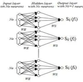
filter and Broad-band e-plane filters with improved stop-band).We use a multilayer
perceptron neural network (MLP-NN) to three layers. Each sub-net in the NN architecture
shown in Fig. 1, possesses Ne input neurons corresponding to the number of the geometry
parameters of the structures, Nc neurons in the hidden layer and one output associated with
the value of S
ij(
f
k). The entire network consists of k distinct NNs corresponding to a particular
frequency with k determined by the number of approximate points in the frequency interval.
Frequency responses of S parameters obtained in simulations compose the network database. The
connection weight from the neurons of the input layer to the neurons of the hidden layer is WE and the
connection weight from the neurons of the hidden layer to the neurons of the output layer is WS.
Fig. 1. Neural network architecture.
II. TEACHING LEARNING BASED OPTIMIZATION
In 2011, Rao et al. [10], [11] proposed an algorithm, called Teaching-Learning-Based Optimization
(TLBO), based on the traditional Teaching Learning phenomenon of a classroom. TLBO is a
population based algorithm, where a group of students (i.e. learner) is considered as population and the
different subjects offered to the learners are analogous with the different design variables of the
optimization problem. The results of the learner are analogous to the fitness value of the optimization
problem. In 2014, Rao and Patel [9] are improving the basic TLBO to enhance its exploration and
exploitation capacities by introducing the concept of number of teachers and adaptive teaching factor.
By means of this modification, the entire class is split into different groups of learners as per their
level (i.e. results), and an individual teacher is assigned to an individual group of learners. Each
teacher tries to improve the results of his or her assigned group based on two phases: the teacher and
Brazilian Microwave and Optoelectronics Society-SBMO received 0 Month 2012; for review 0 Month 2012; accepted 0 Month 2012 A. Teacher phase
In this phase, learners of each group take their knowledge directly through the teacher, where a
teacher tries to increase the mean result value of the classroom to another value, which is better than,
depending on his or her capability. This follows a random process depending on many factors. In this
work, the value of solution is represented as (Xj,k)S, where j means the j
th
design variable (i.e. subject
taken by the learners), k represents the kth population member (i.e. learner), and S represents the Sth
group. The existing solution is updated according to the following expression
( ′, ) = ( , + ) + �� ∗ ℎ− , � > ℎ (1)
( ′, ) = ( , + ) + �� ∗ − ℎ , � ℎ > (2)
The above equations are for a minimization problem, the reverse is true for a maximization problem.
Dj is the difference between the current mean and the corresponding result of the teacher of that group
for each subject calculated by:
( ) = �� ∗ ( ,�� ℎ� − ∗ ) (3)
Where h ≠ k, Mj is the mean result of each group of learners in each subject and TF is the adaptive
teaching factor in each iteration given by equation:
=
� (4)
B. Learner phase
In this part, each group update the learners’ knowledge with the help of the teacher’s knowledge,
along with the knowledge acquired by the learners during the tutorial hours, according to:
( ′′, ) = ′, + �� ∗ ( ′, − ′,�) + �� ∗ ( � ℎ� − ∗ ′, ) , � ( �′) > ′ (5)
( ′′, ) = ′, + �� ∗ ( ′�− ′, ) + �� ∗ ( � ℎ� − ∗ ′, ) , � ′ > ( �′) (6)
Where EF = exploration factor = round (1 + rand).The above equations are for a minimization
problem, the reverse is true for a maximization problem.
III. IMPROVED NEURAL NETWORKS
The training of neural networks is to find an algorithm for optimized weights of networks to
minimize the mean square error (MSE) described as follows
= � ∗ ∑∑ −
� ��
(7)
Where PT the total number of training samples, YS is the output of the network and Y is the desired
output.
= ∑ ∗
�
(∑ ∗
��
) (8)
With f2 and f1are the activation functions (typically: sigmoid, tanh ...), X is the input vector of NN.
Regarding the NN training, the most used training algorithm is the back-propagation (BP)
Brazilian Microwave and Optoelectronics Society-SBMO received 0 Month 2012; for review 0 Month 2012; accepted 0 Month 2012
neural network based on a recently proposed algorithm called Teaching-Learning Based Optimization
(TLBO) [9]; the details of this strategy are presented in the next section.
A. Implementation of TLBO on the neural networks
The step-wise procedure for the implementation of (TLBO-NN) is given in this section.
Step.1. Define the neural network architecture (number of neurons in input layer Ne, number of
neurons in hidden layer Nc and number of neurons in output layer Ns) and define the optimization
problem:
-Design variables of the optimization problem (i.e. number of subjects offered to the learner): WE and
WS the matrices of input connection weights and output connection weights respectively. WE matrix
of Nc rows and Ne columns and WS matrix of Ns rows and Nc columns.
-The optimization problem (fitness function): find the optimal WE and WS which minimizes the mean
square error (MSE) equation(7).
Step.2. Initialize the optimization parameters and initialize the population
-Population size (number of learners in a class) NP
-Number of generations (maximum number of allowable iterations) maxit
-Number of teachers NT
-The initial population according to the population size and the number of neurons and evaluate the
corresponding objective function value. For simplification, the population is decomposed into two
groups one represents the inputs weights population WEp and the second one represents the output
weights population WSp.
� = �� ∗ � ∗ , (9)
� = �� ∗ , � ∗ (10)
Step.3. Select the best solution who acts as chief teacher for that cycle, and select randomly the other
teachers.
Step.4. Arranged the teachers according to their fitness value, then assigns the learners to the teachers
[9].
Step.5. Calculate the mean result of each group of learners in each design variables: MWE, MWS.
Step.6. For each group, evaluate the difference between the current mean and the corresponding result
of the teacher of that group for each design variables by utilizing the adaptive teaching factor [12].
given by equation(4).
Step.7. For each group, update the solution using teacher- phase equations (1) (2), and learner-phase
equations (5) (6).
Step.8. Combine all the groups.
Step.9. Repeat the procedure from step 3 to 8 until the termination criterion is met.
B. Application examples and results
In this part, the performance of the improved neural networks (INN) is investigated for modeling
Brazilian Microwave and Optoelectronics Society-SBMO received 0 Month 2012; for review 0 Month 2012; accepted 0 Month 2012
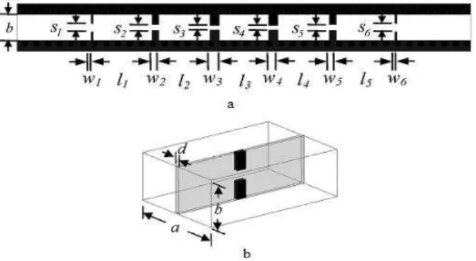
improved stop-band Fig. 3 [14]. The dimensions of the first and second filters are listed in Table I and
Table II respectively.
Fig. 2. The pseudo-elliptic waveguide filter, a) Top view, b) Side cross section view.
Fig. 3. Broad-band E-plane filter, a) The designs of broad-band E-plane filter, b) Fin-line post structure.
TABLE I. DIMENSIONS FOR THE DESIGNED FILTER (UNITS: MILLIMETERS).
a 22.86 b 10.16 l1 3.18 l2 21.43 l3 15.39 l4 15.56 l5 20.43 l6 14.31 V1 4.78 V2 6.86 h1 3.10 h2 3.28 W1 11.37 W2 9.93 W3 11.04
TABLE II. DIMENSIONS FOR THE DESIGNED FILTER (UNITS: MILLIMETERS).
a 7.112 b 3.556 W1 0.254 W2 0.889 W3 1.219 W4 W3 W5 W2 W6 W1 S1 1.092 S2 0.610 S3 0.508 S4 S3 S5 S2 S6 S1 l1 7.696 l2 6.452 l3 6.706 l4 l2 l5 l1 d 0.254
For modeling the two structures above-mentioned. We propose multilayer feed-forward neural
network architecture with a single hidden layer. We begin by selecting the input parameters and
creating database, the latter starts by creating a list of points from the matrix of bounds of the input
parameters. The list of the database points is of size (Ne, PNe), Ne is the number of input parameters,
Brazilian Microwave and Optoelectronics Society-SBMO received 0 Month 2012; for review 0 Month 2012; accepted 0 Month 2012
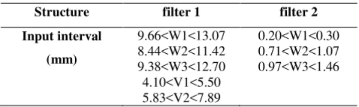
for each variable P=4, Ne=5 for the first filter corresponding to (W1, W2, W3, V1, V2) with a
database equal 1024 and Ne=3 for the second filter corresponding to (W1, W2, W3) with a database
equal 64. The bounds of each parameter are presented in Table III. The number of output Ns=1
corresponding to the frequency responses of the Sij parameters. For the frequency range, we chose to
be (8, 12 GHz) with a number of points K=41 and (26, 36 GHz) with K=34 for the first and the second
filter respectively. The choice of the number of hidden neurons is strongly related to the nature of
non-linearity to model. In our application examples, the number of hidden neurons gives a good
convergence of the algorithm and a good accuracy of the neural model formed are Nc=8 for the first
filter and Nc=6 for the second filter. The activation functions are hyperbolic tangent function (Tansig),
and linear function (Purelin) respectively. When the architecture of NN is selected, the next step is to
train NN using TLBO algorithm section (III. A). We begin by initializing the connection weights
equations (9) and (10). Once the learning is complete, we obtained the update WE and WS and we
can approximate the S parameters response to any input parameter in the boundary range using
equation (8).
TABLE III. INPUT PARAMETERS AND THEIR LIMITS
Structure filter 1 filter 2
Input interval
(mm)
9.66<W1<13.07 8.44<W2<11.42 9.38<W3<12.70 4.10<V1<5.50 5.83<V2<7.89
0.20<W1<0.30 0.71<W2<1.07 0.97<W3<1.46
Fig. 4 and Table IV shows the convergence of PSO and TLBO algorithms for minimize the MSE of
NN for the filters above-mentioned with the effect of the number of teachers in TLBO algorithm. The
common parameters for algorithms (population size NP=50, number of iterations is 300 for the first
filter, and 100 for the second filter), the other specific parameters of the algorithms are given below.
PSO Settings: c and c are constant coefficients c = c = , w is the inertia weight decreased linearly from 0.9 to 0.2.
Brazilian Microwave and Optoelectronics Society-SBMO received 0 Month 2012; for review 0 Month 2012; accepted 0 Month 2012 Fig. 4. Convergence of algorithms for minimizing the MSE, a) first filter, b) second filter.
TABLE IV. COMPARATIVE RESULTS OF CONVERGENCE OF MSE
Structure Filter 1 Filter 2
MSE Best Worst Mean Best Worst Mean
PSO 0.1231 0.5218 0.2731 0.2342 1.0401 0.4666
TLBO
NT=3 0.0521 0.3292 0.1281 0.1289 0.3571 0.1934
NT=5 0.0219 0.2919 0.1059 0.0903 0.2692 0.1718
NT=7 0.0142 0.2686 0.0898 0.0196 0.1402 0.0844
It is observed from Fig. 4 and Table IV that, the TLBO (NT=7) algorithm perform better in terms of
convergence than the PSO algorithm, in which this algorithm requires less number of iterations to
converge to optimum solution as compared to PSO algorithm. Fig.5 and Fig.6 gives the approximate
parameters S11, S21 (magnitude and phase) for the first and second filters respectively, an excellent
approximate can be observed.
Brazilian Microwave and Optoelectronics Society-SBMO received 0 Month 2012; for review 0 Month 2012; accepted 0 Month 2012 Fig. 6. The approximate parameters S11, S21 (magnitude and phase) for the second filter
IV. CONCLUSION
In this paper, Teaching–Learning-Based Optimization (TLBO) algorithm is proposed to training and
testing feed-forward neural networks (FNN) for modeling waveguide filter structures (Pseudo-elliptic
waveguide filter and Broad-band E-plane filters with improved stop-band). The results show the
efficiency of TLBO algorithm, where TLBO algorithm converges to the global minimum faster than
PSO algorithm. The main advantage of this algorithm does not require selection of the
algorithm-specific parameters.
REFERENCES
[1] S.M. Ali, N.K. Nikolova, and M.H. Bakr, “Sensitivity Analysis with Full-Wave Electromagnetic Solvers Based on Structured Grids,” IEEE Transactions on Magnetics, vol.40 ,pp.1521–1529, 2004.
[2] Y. Wang, M. Yu, H. Kabir, and Q.J. Zhang, “Application of Neural Networks in Space Mapping Optimization of Microwave Filters,” International Journal of RF and Microwave Computer Aided Engineering, vol. 22, pp. 159–166, 2012.
[3] J. S. Sivia, A. P. S. Pharwaha, and T. S. Kamal, “Analysis and Design of Circular Fractal Antenna Using Artificial Neural Networks,” Progress in Electromagnetics Research B, vol. 56, pp. 251– 267, 2013.
[4] A. A. Deshmukh, S.D. Kulkarni, A.P.C. Venkata, and N.V. Phatak, “Artificial Neural Network Model for Suspended
Rectangular Microstrip Antennas,” Procedia Computer Science, vol. 49, pp. 332–339, 2015
[5] D.J. Jwo, and K.P. Chin, “ Applying Back-propagation Neural Networks to GDOP Approximation,” The Journal of Navigation, vol. 55, pp. 97–108, 2002.
[6] D. Gyanesh, K. P. Prasant, and K. P. Sasmita, “Artificial Neural Network Trained by Particle Swarm Optimization for Non-Linear Channel Equalization,” Expert Systems with Applications, vol. 41, pp. 3491–3496, 2014.
[7] S. Ding, Y. Zhang, J. Chen, and J. Weikuan, “Research on Using Genetic Algorithms to Optimize Elman Neural Networks,” Neural Computing and Applications, vol.23, pp. 293–297, 2013.
[8] K. Khan, and A. Sahai, “A Comparison of BA, GA, PSO, BP and LM for Training Feed Forward Neural Networks in E -Learning Context,” International Journal of Intelligent Systems and Applications, vol.4, pp. 23 – 29, 2012.
[9] R. V. Rao, V. Patel , “An improved teaching-learning-based optimization algorithm for solving unconstrained optimization problems,” Scientia Iranica ,vol 20, pp. 710–720, 2014.
[10] R.V. Rao, V. J. Savsani, and D. P. Vakharia, “Teaching–Learning-Based Optimization: A Novel Method for Constrained Mechanical Design Optimization Problems,” Computer-Aided Design, vol.43, pp. 303–315, 2011.
[11] R.V. Rao, V. J. Savsani, and D. P. Vakharia, “Teaching–Learning-Based Optimization: An Optimization Method for Continuous Non-Linear Large Scale Problems,” Information Sciences, vol.183, pp. 1–15, 2012.
[12] R. V. Rao , D. P. Rai, “Optimization of fused deposition modeling process using teaching-learning-based optimization algorithm,” Engineering Science and Technology, an International Journal , 19, pp. 587–603, 2016.
[13] Q. Zhang, and Y. Lu, “Design of Wide-Band Pseudo-Elliptic Waveguide Filters with Cavity-Backed Inverters,”IEEE Microwave And Wireless Components Letters, vol.20 ,pp. 604–606, 2010.