www.biogeosciences.net/13/5021/2016/ doi:10.5194/bg-13-5021-2016
© Author(s) 2016. CC Attribution 3.0 License.
Biogeochemical modeling of CO
2
and CH
4
production
in anoxic Arctic soil microcosms
Guoping Tang1, Jianqiu Zheng2, Xiaofeng Xu3, Ziming Yang1, David E. Graham2,4, Baohua Gu1, Scott L. Painter1,4, and Peter E. Thornton1,4
1Environmental Sciences Division, Oak Ridge National Laboratory, Oak Ridge, TN 37831, USA 2Biosciences Sciences Division, Oak Ridge National Laboratory, Oak Ridge, TN 37831, USA 3Biology Department, San Diego State University, San Diego, CA 92182, USA
4Climate Change Science Institute, Oak Ridge National Laboratory, Oak Ridge, TN 37831, USA
Correspondence to:Guoping Tang ([email protected])
Received: 13 May 2016 – Published in Biogeosciences Discuss.: 20 May 2016
Revised: 20 August 2016 – Accepted: 24 August 2016 – Published: 12 September 2016
Abstract. Soil organic carbon turnover to CO2and CH4 is sensitive to soil redox potential and pH conditions. How-ever, land surface models do not consider redox and pH in the aqueous phase explicitly, thereby limiting their use for making predictions in anoxic environments. Using re-cent data from incubations of Arctic soils, we extend the Community Land Model with coupled carbon and nitro-gen (CLM-CN) decomposition cascade to include simple organic substrate turnover, fermentation, Fe(III) reduction, and methanogenesis reactions, and assess the efficacy of various temperature and pH response functions. Incorporat-ing the Windermere Humic Aqueous Model (WHAM) en-ables us to approximately describe the observed pH evolu-tion without addievolu-tional parameterizaevolu-tion. Although Fe(III) reduction is normally assumed to compete with methano-genesis, the model predicts that Fe(III) reduction raises the pH from acidic to neutral, thereby reducing environmental stress to methanogens and accelerating methane production when substrates are not limiting. The equilibrium specia-tion predicts a substantial increase in CO2 solubility as pH increases, and taking into account CO2 adsorption to sur-face sites of metal oxides further decreases the predicted headspace gas-phase fraction at low pH. Without adequate representation of these speciation reactions, as well as the impacts of pH, temperature, and pressure, the CO2 produc-tion from closed microcosms can be substantially underes-timated based on headspace CO2 measurements only. Our results demonstrate the efficacy of geochemical models for simulating soil biogeochemistry and provide predictive
un-derstanding and mechanistic representations that can be in-corporated into land surface models to improve climate pre-dictions.
1 Introduction
Global warming is expected to accelerate permafrost thaw, which may trigger the release of the large amount of frozen soil organic matter (SOM) stored in the Arctic as carbon dioxide (CO2)and methane (CH4)into the atmosphere, pos-sibly forming a positive feedback to climate change (Treat et al., 2015; Knoblauch et al., 2013; Elberling et al., 2013). Permafrost thawing leads to significant changes in soil water saturation, creating favorable conditions for anaerobic respi-ration and methanogenesis (Lawrence et al., 2015).
Schädel et al., 2016). However, in incubations with soils from Alaska and Siberia, carbon release under aerobic conditions was 3.9–10 times greater than under anaerobic conditions (Lee et al., 2012), and CO2production appeared ceased at late times in anaerobic microcosms (Xu et al., 2015; Roy Chowdhury et al., 2015), indicating that these existing mod-els do not adequately represent the anaerobic processes for accurate prediction of SOM turnover and heterotrophic res-piration.
In addition, it is important to accurately represent methanogenesis in the context of competing anaerobic pro-cesses because CH4has a 100-year global warming potential that is about 26 times greater than CO2(Forster et al., 2007; IPCC, 2013) and an atmospheric residence time of approxi-mately 10 years (IPCC, 2013), and methanogenesis rate can be high under favorable conditions. Methanogenesis is car-ried out by a group of strictly anaerobic archaea. The free energy of methanogenesis reactions is less favorable than the reduction of O2, NO−
3, Mn (IV), Fe(III), and SO24−along the redox ladder (Conrad, 1996; Bethke et al., 2011). The ac-cumulation of CH4has been widely observed to lag behind CO2 for periods ranging from days to years in incubations (Knoblauch et al., 2013; Roy Chowdhury et al., 2015; Cui et al., 2015; Hoj et al., 2007; Fey et al., 2004; Jerman et al., 2009; Tang et al., 2013c). The implication is that a first-order representation (including constant CO2/ CH4ratio parame-terization) normally overpredicts CH4production rate before methanogenesis initiation and underpredicts CH4production rate afterwards, and the uncertain lag time introduces large bias in CH4production prediction.
Besides temperature (Fey and Conrad, 2003; Hoj et al., 2007; Jerman et al., 2009; Cui et al., 2015) and initial methanogen abundance (Conrad, 1996; Knoblauch et al., 2013), the wide range of redox buffers provided by the alter-native electron acceptors is likely a cause of the wide range of observed lag times (Estop-Aragonés and Blodau, 2012; Fey et al., 2004; Jerman et al., 2009; Yao et al., 1999; Con-rad, 1996; Knorr and Blodau, 2009). As a result, the ratio of CH4 to CO2 ranges from 0.00001 to 0.5 (Wania et al., 2010; Drake et al., 2009; Bridgham et al., 2013), highlighting the limitation of the CH4/ CO2ratio approach. Nevertheless, some land surface models (LSMs) parameterize methano-genesis as a fraction of carbon mineralization (Wania et al., 2013; Oleson et al., 2013; Koven et al., 2015; Cheng et al., 2013). While methanogenesis is explicitly represented in some models (Xu et al., 2015; Grant, 1998) and the reduction of alternative electron acceptors is explicitly represented in others (Fumoto et al., 2008; Segers and Kengen, 1998; van Bodegom et al., 2000, 2001), these models do not have an aqueous phase that is essential for explicit biogeochemical calculations, e.g., pH, Eh, and thermodynamic calculations. Because methanogenesis is sensitive to redox conditions, the lack of explicit biogeochemical representation of the redox processes contributes to the prediction uncertainty of CH4 emission.
Anaerobic bacteria and archaea usually depend on sim-ple substrates such as sugars, alcohols, organic acids, and H2 as carbon and energy sources that are rarely simulated in ecosystem models (Manzoni and Porporato, 2009; Xu et al., 2015). Instead, they are typically lumped together as dissolved organic matter (DOM) or low-molecular-weight organic carbon (LMWOC) (e.g., Tian et al., 2010). The abundance and importance of DOM and LMWOC in SOM turnover in the Arctic soils are becoming increasingly rec-ognized (Hodgkins et al., 2014). The DOM concentration in water flowing from collapsing permafrost (thermokarsts) on the North Slope of Alaska ranges from 0.2 to 8 mM, with biodegradable (degrading in 40 days) DOM accounting for 10–60 % (Abbott et al., 2014; Arnosti, 1998, 2000; Arnosti et al., 1998). Ancient LMWOC was found to fuel rapid CO2 production upon thawing (Drake et al., 2015). On the other hand, new SOM consists of mostly macromolecules of plant and microbial residues such as carbohydrates (polysaccha-rides, including cellulose and hemicellulose), lipids, nucleic acids, and proteins (Kögel-Knabner, 2002). While concep-tual models and measurements connecting SOM with LM-WOC have long existed (Drake et al., 2009; Tveit et al., 2013, 2015; Bridgham et al., 2013), the hydrolysis and fermenta-tion reacfermenta-tions have been poorly represented and quantified in the Arctic as well as temperate and tropical soils. Among over 250 SOM decomposition models that have been devel-oped in the past 80 years (Manzoni and Porporato, 2009), only a few models explicitly simulate simple substrates (Xu et al., 2016b). Either a simple carbon pool (Cao et al., 1995, 1998; Kettunen, 2003) or a DOM pool (Tian et al., 2010; Xu and Tian, 2012) has been assumed for methanogene-sis. The production of acetate and H2 has been parameter-ized as a function of carbon mineralization (van Bodegom et al., 2000, 2001; Grant, 1998; Xu et al., 2015). It is not sur-prising that CH4production prediction is sensitive to simple substrate production (Kettunen, 2003; Weedon et al., 2013). While detailed SOM decomposition models include depoly-merization to produce monomers under aerobic conditions (Riley et al., 2014), production and consumption of simple measurable substrates, such as acetate, H2, and formate, are not explicitly represented under anaerobic conditions.
(Ole-son et al., 2013; Tian et al., 2010). pH is calculated using soil acidity and soil buffer capacity (van Bodegom et al., 2001) or as a function of acetate concentration (Xu et al., 2015). It is desirable to use a geochemical model to describe pH evo-lution mechanistically. The pH response functions (reaction rate adjustment factor as a function of pH) in LSMs are em-pirical and vary substantially (Xu et al., 2016b). Assessing the efficacy of these functions is needed to better represent pH impacts on carbon mineralization and methanogenesis.
Temperature is another critical factor controlling SOM turnover to CO2 and CH4. The reported Q10 values for methanogen temperature response vary from 1.5 to 4 (Xu et al., 2016b). Methanogenesis has been widely observed to diminish when the temperature decreases toward 0◦C (Dun-field et al., 1993; Fey et al., 2004; Hoj et al., 2007; Sow-ers et al., 1984), predicting little CH4 production from the surface layers of frozen Arctic soils. However, recent obser-vations suggest that CH4 emissions during the winter sea-son account for ≥50 % of the annual emission in the
Arc-tic (Zona et al., 2016). The cold-season CH4 production is among the most uncertain processes for predicting seasonal CH4cycle in northern wetlands (Xu et al., 2016a). The tem-perature response functions (reaction rate adjustment factor as a function of temperature) need to be assessed as well.
Overall, anaerobic SOM turnover is controlled by the hy-drolysis of the macromolecules to produce simple substrates and the sequential microbial reduction of electron acceptors along the redox ladder. Because SOM turnover and CO2and CH4 productions are sensitive to redox potential, pH, and temperature, it is desirable to simulate the redox and pH explicitly with geochemical models. With the accumulation of new data on metabolic intermediates, electron acceptors, greenhouse gases, and pH from incubations with Arctic soils at various temperatures (Drake et al., 2015; Herndon et al., 2015a, b; Yang et al., 2016; Mann et al., 2015), our objec-tives are to integrate these new data into geochemical models to (1) extend the CLM-CN decomposition cascade to include simple substrates such as sugars and organic acids and add Fe(III) reduction and methanogenesis processes; (2) account for gas-, aqueous-, and adsorbed-phase speciation; (3) de-scribe pH mechanistically; and (4) assess the existing tem-perature and pH response functions. Unlike with previous LSMs, we simulate speciation of CO2and CH4in the gas, aqueous, and solid phases, and represent sugars, organic acids, Fe(II), Fe(III), Fe reducers, and methanogens, and ac-count for both thermodynamic and kinetic control. Our re-sults provide predictive understanding and mechanistic rep-resentations that can be incorporated in LSMs, e.g., CLM-PFLOTRAN (Tang et al., 2016), to improve climate model predictions.
The carbon cycle involves coupled hydrological, geo-chemical, and biological processes interacting from molec-ular to global scales. The implicit empirical first-order ap-proach used in existing LSMs limits our understanding of the land atmosphere interaction and is a source of prediction
uncertainty. To improve our understanding and reduce pre-diction uncertainty, we attempt to use relatively more explicit mechanistic representations developed in the reactive trans-port model literature (Tang et al., 2016). Even though ex-plicit representation does not necessarily improve the match between the predictions and observations over well-tuned ex-isting models immediately (e.g., Wieder et al., 2015; Steven et al., 2006), our approach provides a systematic means to incorporate ongoing process-rich investigations to improve mechanistic representations in LSMs across scales. For a pre-liminary study, we constrain our scope to extending CLM-CN with minimum revision to describe anaerobic CO2 and CH4 production from several recent microcosm studies in this work. We discuss the next steps briefly in the “Results and discussion” section.
2 Materials and methods
We extend the CLM-CN decomposition cascade (Thornton and Rosenbloom, 2005) by adding reactions for hydroly-sis to produce sugars, fermentation to produce organic acids and H2 (Grant, 1998; Xu et al., 2015), Fe(III) reduction, and methanogenesis reactions (Tang et al., 2013c). We add the Windermere Humic Aqueous Model (WHAM) (Tipping, 1994) to simulate the pH buffer by SOM. Recent microcosm data (Herndon et al., 2015a; Roy Chowdhury et al., 2015) are used to assess these representations. While nitrogen (am-monium and nitrate) concentrations can affect carbon min-eralization (Lavoie et al., 2011), we do not account for this effect because of a lack of nitrogen measurements from these experiments.
2.1 Soil incubation experiment data
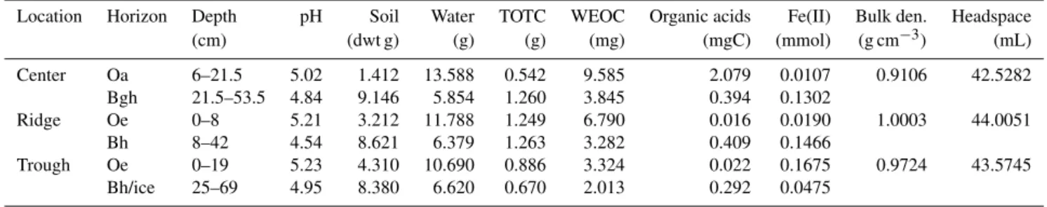
The materials, experimental procedures, and results for the microcosm tests have been reported previously (Herndon et al., 2015a; Roy Chowdhury et al., 2015). Briefly, three soil cores were taken from center, ridge, and trough locations in a low-center polygon (a typical Arctic geographic feature in the low lands with soils surround by ice wedges; see cited references for more information) in the wet tundra of the Barrow Environmental Observatory in Alaska. Soil samples from the organic and mineral horizons of the three cores were analyzed for gravimetric water content, pH, Fe(II), water-extractable organic carbon (WEOC), organic acids, and to-tal organic carbon content (TOTC). For each horizon and lo-cation, about 15 g of homogenized wet soil was placed into a 60 mL sterile serum bottle, which was sealed and flushed with pure N2 gas. The microcosms were incubated at −2,
and organic acids. Additional soil characterization is avail-able elsewhere (Bockheim et al., 2001; Lipson et al., 2010, 2013b).
2.2 Model developments
2.2.1 SOM decomposition
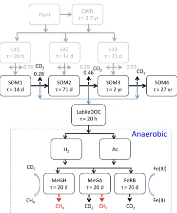
The SOM in the Arctic soils was characterized using high-resolution mass spectroscopy (Herndon et al., 2015a; Mann et al., 2015; Hodgkins et al., 2014). However, these char-acterizations were insufficient to partition SOM into many chemically distinct organic pools (Riley et al., 2014; Kögel-Knabner, 2002). Therefore, we extend the CLM-CN de-composition cascade to produce intermediate metabolites (Fig. 1). To limit the number of new pools, we lump reduc-ing sugars, alcohols, etc. (Yang et al., 2016; Kotsyurbenko et al., 1993; Glissmann and Conrad, 2002; Tveit et al., 2015) into a labile DOC pool (LabileDOC), and the organic acids, such as formate, acetate, propionate, and butyrate (Herndon et al., 2015a; Kotsyurbenko et al., 1993; Peters and Conrad, 1996; Tveit et al., 2015) into an organic acid pool (Ac) (Xu et al., 2015; Grant, 1998). Assuming that the labile DOC turns over in 20 h like the Lit1 pool in CLM-CN (Thornton and Rosenbloom, 2005) or glucose fermentation (Rittmann and McCarty, 2001), we split the original respiration factor into a direct and an indirect fraction, with the indirect frac-tionslabileto produce labile DOC, which respires through the anaerobic pathway (Fig. 1) to CO2 or CH4, and the direct respiration fraction (1−slabile)respires directly to CO2. We estimateslabile by comparing the predictions with the obser-vations in this work. The fermentation reaction is (Xu et al., 2015; Grant, 1998; van Bodegom and Scholten, 2001; Madi-gan, 2012)
C6H12O6+4H2O→2CH3COO−+2HCO−3+4H++4H2, (R1)
which lowers the pH and further respires slabile/3 of SOM into CO2.
2.2.2 Fe(III) reduction, methanogenesis, and biomass decay
Because Fe(III) reduction contributes 40–45 % of the ecosys-tem respiration in some Arctic sites (Lipson et al., 2013b) and NO−
3 and SO24−concentrations are typically low in the experiments, we add Fe(III) reduction reactions to represent the reduction of alternative electron acceptors to O2. We use the microbial reactions formed by combining electron donor (oxidation) half reactions, electron acceptor (reduction) half reactions, and cell synthesis reactions following bioenerget-ics (Rittmann and McCarty, 2001). Specifically, the Fe(III)
Lit1
τ = 20 h
SOM1
τ= 14 d
SOM2
τ= 71 d
SOM3
τ= 2 yr
Lit2
τ= 14 d
Lit3
τ= 71 d
SOM4
τ= 27 yr
Plant
0.39 0.29
0.28 0.46
0.55 CWD
τ= 2.7 yr
LabileDOC
τ= 20 h
MeGH
τ= 20 d
MeGA
τ= 20 d
FeRB
τ= 20 d
H2 Ac
Fe(III)
Fe(II) CO2
CH4
CH4 CO2 CH4
Anaerobic
CO2
CO2
CO2
CO2
Figure 1. Extension of the CLM-CN decomposition cascade
(Thornton and Rosenbloom, 2005) to include a labile DOC pool (LabileDOC). A portion of the original respiration fraction is as-sumed to produce labile DOC, which undergoes fermentation, Fe reduction, and methanogenesis to release CO2 and CH4. FeRB,
MeGA, and MeGH denote microbial mass pools for Fe reducers, acetoclastic methanogens, and hydrogenotrophic methanogens, re-spectively.τis the turnover time.
reduction reactions are (Istok et al., 2010) 2.1H2O+NH+4 +150.2Fe3++21.3CH3COO−
→ C5H7O2N+150.2Fe2+
+167.4H++37.5HCO−3, (R2)
5HCO3−+NH+4 +114.8Fe3++57.4H2 → C5H7O2N+114.8Fe2+
+110.8H++13H2O, (R3)
where C5H7O2N represents microbial (iron reducer) mass, and NH+
4 is assumed not to be limiting (at 1 µM). These two reactions result in dissolution of ferric oxides, for example, Fe(OH)3a, to release OH−to increase pH. The rate is dx
dt =kmaxx
ksurf ksurf+x/msurf,avail
mD
kD+mDf (G), (1) wherekmax is the kinetic rate constant; x is concentration of biomass; msurf,avail is the microbially available surface sites taken as the Fe(OH)3a surface sites Hfo (hydrous fer-ric oxides) associated with H+, i.e.,m
mHfo_sOH in moles per liter of pore fluid;ksurfaccounts for the impact ofx/msurf,avail, which represents the interaction of biomass with available Fe(III) sites on the surface;mDand kD are the concentration and half saturation of the electron donors (acetate or H2); andf (G)is a thermodynamic fac-tor that goes to zero when the reaction is thermodynamically unfavorable (Jin and Roden, 2011).
The methanogenesis reactions are (Istok et al., 2010) 1.5H++98.2H
2O+NH+4 +103.7CH3COO−
→C5H7O2N+101.2HCO−3 +101.2CH4, (R4) 84.9H+
+NH+4 +85.9HCO−3 +333.5H2
→C5H7O2N+255.6H2O+80.9CH4. (R5) These two reactions consume protons to increase pH. The rate is
dx
dt =kmaxx mD
kD+mDf (G). (2)
We use one pool, FeRB, for the iron reducers and separate the methanogens into the MeGA and MeGH pools for acetoclas-tic and hydrogenotrophic methanogens (Fig. 1). The biomass decay reaction for FeRB, MeGA, and MeGH is
0.2C5H7O2N→ 0.1SOM1+0.2SOM2+0.25SOM3 +0.45SOM4+0.1185NH+4 +. . . (R6) Like the SOM pools, the rate is first order.
In this model, iron reducers and methanogens interact in different ways under various conditions. When the electron donors (acetate and H2)are abundant, iron reducers grow faster than methanogens when Fe(III) is not limiting (de-pending on the Fe(OH)3asurface sites and iron reducers pop-ulation), i.e., iron reducers have a short doubling time than methanogens. When the electron donors are limiting, iron re-ducers are expected to outcompete methanogens, depending on the half-saturation (substrate affinity) values. The model also accounts for the thermodynamics. However, it does not account for possible different responses to temperatures and pH for iron reducers and methanogens.
2.2.3 pH
The soil pH is typically buffered by carbonates, clay miner-als, metal oxides, and organic matter (Tipping, 1994; Tang et al., 2013a). The Windermere Humic Aqueous Model (WHAM) is used to approximate SOM as humic acid and fulvic acid, with a number of monodentate and bidentate binding sites for protons, to describe the pH buffering due to SOM (Tipping, 1994). The surface complexation model for ferrihydrate is used to describe the sorption of carbonate and proton to metal oxides (Dzombak and Morel, 1990). Ad-ditional aqueous speciation reactions are also included in the reaction database available in the Supplement (also publicly available at https://github.com/t6g/bgcs).
2.2.4 pH and temperature response functions
We use the CLM4Me pH response function (Riley et al., 2011; Meng et al., 2012)
log10f (pH)= −0.2235pH2+2.7727pH−8.6 (3)
and the CLM-CN temperature response function (Thornton and Rosenbloom, 2005; Lloyd and Taylor, 1994)
lnf (T )=308.56
1
71.02− 1 T−227.13
. (4)
The pH response functions used in DLEM (Tian et al., 2010) and TEM (Raich et al., 1991) and a few other models (Cao et al., 1995; Xu et al., 2015), as described in Appendix A, and the CENTURY temperature response function, theQ10 equation, the Arrhenius equation, and the Ratkowsky equa-tion, which are described in Appendix B, are used for com-parison.
2.3 Implementation, parameterization, and initialization
2.3.1 Implementation
To calculate the speciation of CO2, CH4, H2, Fe, etc. among gas, aqueous, and solid phases under various temperature, pH, and pressure conditions and explicitly describe pH and redox buffer, we employ the widely used extensively tested geochemical code PHREEQC (Parkhurst and Appelo, 2013) to synthesize the experimental data to develop and param-eterize mechanistic representations. The implementation of CLM-CN reactions in a geochemical code is detailed else-where (Tang et al., 2016). Guidelines for implementation of the microbial reactions, surface complexation, WHAM, etc. in PHREEQC are available in the user manual (Parkhurst and Appelo, 2013).
2.3.2 Parameterization
The stoichiometric and kinetic rate parameters for the CLM-CN reaction network are specified in Fig. 1. The indirect respiration factionslabile is highly uncertain. We start with slabile=0.4 and check the sensitivity with slabile=0.2 and
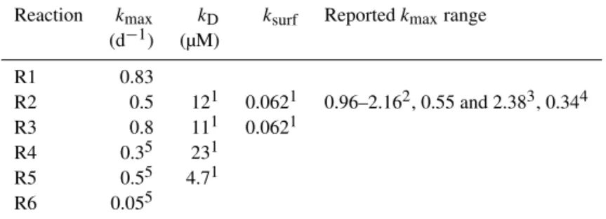
0.6. For the decay of biomass, and growth of methanogens, we use the general parameter values in the literature (Rittmann and McCarty, 2001). The half-saturationkD and ksurf values are taken from the literature as well (Jin and Roden, 2011). The parameter values and the references are listed in Table 1.
2.3.3 Initialization
Table 1.Model parameter values for base scenario.
Reaction kmax kD ksurf Reportedkmaxrange
(d−1) (µM)
R1 0.83
R2 0.5 121 0.0621 0.96–2.162, 0.55 and 2.383, 0.344
R3 0.8 111 0.0621
R4 0.35 231
R5 0.55 4.71
R6 0.055
1Jin and Roden (2011);2Esteve-Núñez et al. (2005);3Cord-Ruwisch et al. (1998);4Holmes et al. (2013);5Rittmann and McCarty (2001).
(combined formate, acetate, propionate, and butyrate from Table S1 to Table 2), and Fe(II) concentration are specified as measured.
The measured total organic carbon includes seven carbon pools in the CLM-CN decomposition cascade, as well as sim-ple substrates (such as sugars, alcohols, and organic acids), and biomass for FeRB, MeGA, MeGH, and other microbes. Because of the lack of reliable methods in partitioning the measured total organic carbon into these pools, we com-bine the Lit1 pool with LabileDOC, Lit2 with SOM1, and Lit3 with SOM2 pools as they have identical turnover times (Fig. 1). That is, we will split the initial total organic carbon (minus simple substrates) into LabileDOC, SOM1, SOM2, SOM3, SOM4, FeRB, MeGA, and MeGH pools, with fraction fLabileDOC, fSOM1, fSOM2, fSOM3, fFeRB, fMeGA, and fMeGH(the rest is fSOM4, i.e.,fSOM4=1–fLabileDOC–
fSOM1–fSOM2–fSOM3–fFeRB–fMeGA–fMeGH). Because the experiments lasted for only 2 months, and predictions are often not very sensitive to the initial biomass (Tang et al., 2013b, c; Xu et al., 2015; Jin and Roden, 2011), the predic-tions are expected to be sensitive to fLabileDOC,fSOM1, and fSOM2 under the experimental conditions (as the turnover times for SOM3 and SOM4 are 2 and 27 years, respec-tively; Fig. 1). With a turnover (mean residence) time of 0.2–0.5, 6–9, and > 125 years for the fast, slow, and pas-sive pools, respectively, less than 5 % was estimated for the fast pool for 121 individual samples from 23 high-latitude ecosystems located across the northern circum-polar permafrost zone (Schädel et al., 2014). Based on incubation tests with Siberian soils for over 1200 days, the initial labile carbon pools were estimated to comprise 2.22±1.19 and 0.64±0.28 % of the total organic carbon
with turnover times of 0.26±1.56 and 0.21±1.58 years
under aerobic and anaerobic conditions, respectively (Knoblauch et al., 2013). We set fLabileDOC=0.0005,
fSOM1=0.01, fSOM2=0.02, fSOM3=0.1, fbio=10−6,
fMeGA=fMeGH=fbio, and fFeRB=2fbio (approximating
withE. coliwith a wet weight 10−12g, 70 % water, and 50 % dry weight carbon (Madigan, 2012), each microbial cell con-tains∼1.25× 10⁻¹⁴mol C;fbio=10−6means∼108cells
in 1 mol of total organic carbon, which roughly approximates the range of reported values in Roy Chowdhury et al., 2015). Bioavailable ferric oxides are assumed to be in the form of Fe(OH)3a, with initial concentration as a fraction fFe3 of the dry soil mass. Depending on the season and the age of the drained thawed lake basins, HCl extractable Fe(III) is reported to range between 100 and 700 g Fe(III) m−3 in the Barrow soils in a 24 cm soil profile (Lipson et al., 2013a). Using a weighted average of bulk density of 0.26, this translates to 0.2 to 1 % g Fe(III) g−1dry soil mass. While bioavailable Fe(III) in soils is not well defined (e.g., Hy-acinthe et al., 2006; Poulton and Canfield, 2005), we start withfFe3=0.005 and evaluate the sensitivity with a range
of values. Fe(III) reduction dissolves Fe(OH)3aand releases adsorbed protons on the mineral surface, which is described by the surface complexation model (Dzombak and Morel, 1990). The organic content for WHAM is set at total organic carbon. The initial total inorganic carbon (TIC) in the solu-tion is assumed to be in equilibrium with an atmosphere of CO2 at 400 ppm and 1 atm. The headspace gas starts with N2at 1 atm. These parameters are summarized in Table S2. Additional specifics are available in the scripts to produce input files. The reaction database (extended from Tang et al., 2013b, c), the Python scripts to create input files for various locations, temperatures, and other options (e.g., temperature and pH response functions) and scripts used to make the fig-ures are provided in the Supplement.
3 Results and discussion
3.1 Experimental observations
(cen-Table 2.Experimental parameter values summarized from (Herndon et al., 2015; Roy Chowdhury et al., 2015). TOTC: total organic carbon; WEOC: water-extractable organic carbon.
Location Horizon Depth pH Soil Water TOTC WEOC Organic acids Fe(II) Bulk den. Headspace
(cm) (dwt g) (g) (g) (mg) (mgC) (mmol) (g cm−3) (mL)
Center Oa 6–21.5 5.02 1.412 13.588 0.542 9.585 2.079 0.0107 0.9106 42.5282
Bgh 21.5–53.5 4.84 9.146 5.854 1.260 3.845 0.394 0.1302
Ridge Oe 0–8 5.21 3.212 11.788 1.249 6.790 0.016 0.0190 1.0003 44.0051
Bh 8–42 4.54 8.621 6.379 1.263 3.282 0.409 0.1466
Trough Oe 0–19 5.23 4.310 10.690 0.886 3.324 0.022 0.1675 0.9724 43.5745
Bh/ice 25–69 4.95 8.380 6.620 0.670 2.013 0.292 0.0475
ter, ridge, and trough) of ice-wedge polygons. Up to 20 % CO2 was observed in the headspace by the end of the 2-month incubations, with higher concentrations in the organic soils than in the mineral soils (Fig. 2a1–3 vs. Figs. 4–6). This can be attributed to the higher organic content of the organic soils compared to that of the mineral soils (Tables 2, S1).
CO2 in the headspace increased rapidly in the beginning and then the increase slowed (Fig. 2). The initial rapid in-crease can be attributed to fast decomposition of the eas-ily degradable substrates such as sugars and alcohols (Yang et al., 2016; Fey and Conrad, 2003; Glissmann and Con-rad, 2002; Kotsyurbenko et al., 1993). As the easily degrad-able substrates were exhausted, the CO2production rate de-creased. These observations are similar to those for the anaer-obic incubations with soils from a trough location in a high-center polygon at the same site (Yang et al., 2016) and deep Siberian permafrost soils (Knoblauch et al., 2013). However, CO2 continued to increase well beyond 2 months in these previous studies, and the CO2 production rates stabilized, probably reaching a rate limited by the slow rate of hydrol-ysis in the Siberian soil microcosms. These observations are different from the observed CO2level-off in the current mi-crocosms (Fig. 2a2, a4, a5).
CH4 in the headspace increased slowly at the beginning and then accelerated (Fig. 2b1–5), except in the center or-ganic soils. CH4accumulation lagged behind CO2for about 10 days in most of the microcosms and by a few days for the center organic soil microcosms at 4 and 8◦C. These lag times are shorter than those observed in microcosms with deep Siberian permafrost soils (average 960±300 days)
(Knoblauch et al., 2013). This is probably because of the ini-tial abundance of substrates such as organic acids in the Bar-row soils (Fig. 2c1–6). In addition, the shallow BarBar-row soils experience freezing and thawing, and so does microbial ac-tivity every year, while the deep Siberian permafrost soils were frozen for extended periods; as a result, the amount of initial biomass in the shallow Barrow soils is probably much higher than that in the deep Siberian soils.
Organic acids generally accumulated at the beginning, de-creased as CH4concentration increased, and exhausted in the mineral soil microcosms (Fig. 2c1–6). In contrast, organic acids were not exhausted in the center organic soil
micro-cosms (Fig. 2c6). In comparison with similar tests with soils from the high-center polygon trough, organic acids accumu-lated for over 5 months in the organic soils and were not ex-hausted in the mineral soils (Yang et al., 2016). The accumu-lation and disappearance of organic acids have been widely observed in the literature (van Bodegom and Stams, 1999; Fey et al., 2004; Glissmann and Conrad, 2002; Jerman et al., 2009; Kotsyurbenko et al., 1993; Lu et al., 2015; Peters and Conrad, 1996; Yao and Conrad, 1999).
Fe(II) concentrations increased and leveled off (Fig. 2d1– 6), with similar trends for pH (Fig. 2e1–6). The increase in pH concurred with Fe(III) reduction, which released hy-droxides from Fe(OH)3a dissolution. The pH increase is in contrast to the observed pH decrease when Fe(III) reduc-tion was absent (Xu et al., 2015). While Fe(III) reducreduc-tion was reported to inhibit methanogenesis through direct in-hibition (van Bodegom et al., 2004) or substrate competi-tion (Miller et al., 2015; Reiche et al., 2008), the impact ap-pears less significant than expected in these incubations, as well as incubations with the high-center polygon trough soils (Yang et al., 2016). This is consistent with the observation that methane production initiated in the presence of oxidants (Roy et al., 1997). In addition, Fe(III) reduction can both in-hibit and promote methanogenesis (Zhuang et al., 2015). In the Barrow soils, the initial abundance of organic acids prob-ably mitigates the competition between Fe(III) reducing and methanogenic populations, decreasing the lag time between CH4and CO2accumulation.
Substantial microbial activity was observed at −2◦C,
which is above the soil water freezing point due to os-motic and matric potentials. These incubations led to an in-crease in CO2(Fig. 2a1–6), organic acids (Fig. 2c1–6), Fe(II) (Fig. 2d1–6), and pH (Fig. 2e1–6). CH4concentrations were low but detectable in the headspace at−2◦C. The lag time
between CH4 and CO2 increases with decreasing temper-ature, which was widely observed in the literature as well (Fey and Conrad, 2003; Hoj et al., 2007; Jerman et al., 2009; van Bodegom and Scholten, 2001; Fey et al., 2004; Kot-syurbenko et al., 1993; Lu et al., 2015). The transition from
−2 to 4 and 8◦C appears to be gradual, except for the center
organic soils, where CH4increases were drastic from−2 to
re-0
10
20
30
CO
2(%
)
(a1)
Trough
(a2)
idge
Mineral
(a3)
Center
(a4)
Trough
(a5)
RRidge
Organic
(a6)
Center
0
1
2
3
4
CH
4(%
)
(b1)
(b2)
(b3)
(b4)
(b5)
(b6)
0
10
20
Ac (mM)
(c1)
(c2)
(c3)
(c4)
(c5)
(c6)
0
20
40
60
80
Fe(II) (mM)
(d1)
(d2)
(d3)
(d4)
(d5)
(d6)
-2◦C+4◦C +8◦C
0 20 40 60
Time (d)
4
5
6
pH
(e1)
0 20 40 60
Time (d)
(e2)
0 20 40 60
Time (d)
(e3)
0 20 40 60
Time (d)
(e4)
0 20 40 60
Time (d)
(e5)
0 20 40 60
Time (d)
(e6)
R R
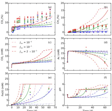
Figure 2.Comparison of observed and modeled CO2(a1–6)and CH4(b1–6)in the headspace, organic acid (Ac,c1–6), extractable Fe(II) (d1–6), and pH(e1–6)in the incubation tests with soils from an Arctic lower-center polygon. Symbols represent observations with blue, green, and red for−2, 4, and 8◦C. For CO2and CH4, different symbols of the same color represent duplicates. The organic acids, such as formate, acetate, propionate, and butyrate, reported by Herndon et al. (2015) are combined as Ac in(c1–6). The rest of the data were
taken from Roy Chowdhury et al. (2015). The curves are calculations based on model parameter values listed in Table 1 and experimental parameter values listed in Table 2. Trough, ridge, and center denote the microtopographic locations in the polygon, and mineral and organic denote soil horizons. Increasing the initial bioavailable Fe(III)fFefrom 0.005 (continuous line) to 0.01 (dashed line) and 0.02 (dash-dotted
line) brings the predictions close to the observations for Fe(II) and pH for center and ridge organic soils.
sponses are diverse, as manifested byQ10values from 1.6 to 22 (Roy Chowdhury et al., 2015).
3.2 Modeling results
3.2.1 Overall
With the same model parameter values given in Table 1 and Table S2 and different experimental parameter values listed in Table 2, the model roughly predicts the observed trends for different soils at the three temperatures (Fig. 2): CO2and CH4accumulate in the headspace; CO2accumulation slows down, while CH4speeds up at later times; CH4lags behind CO2; organic acids accumulate and then decrease; Fe(II) ac-cumulates and levels off; pH increases and levels off; and car-bon mineralization and methanogenesis rates increase with temperature.
While the model predicts little CO2 and CH4 in the headspace at−2◦C, which is similar to what was observed,
it predicts little change in Fe(II) and pH as well, which is not consistent with the observations. To improve the predic-tion at−2◦C, which can be important (Zona et al., 2016; Xu
et al., 2016a), it is necessary to understand why little CO2 or CH4was observed to occur with Fe(III) reduction, which was indicated by the increase in Fe(II) and pH.
stabi-lized as the carbon release became limited likely by hydrol-ysis of polymers. The observed sustained CO2accumulation in these closed microcosms indicates that the observed trends in Fig. 2a1–6 at later times are probably uncertain. Except for these mismatches, the model predictions generally agree with the observations for the mineral soils reasonably well.
In contrast, the predictions do not agree as well with the observations for the organic soils. For the trough or-ganic soils, the model underpredicts CO2 in the headspace (Fig. 2a4) but describes the rest of the observations reason-ably well. In addition to CO2 (Fig. 2a5), the model under-predicts Fe(II) and pH increase in the ridge organic soils (Fig. 2d5, e5). The prediction of the center organic soils dif-fers from the observations the most (last column in Fig. 2). These mismatches might be explained by model biases in ini-tial Fe(III) content, labile DOC, and biomasses.
3.2.2 Fe(III) reduction
Agreement between predictions and observations for the Fe(II) and pH increase can be improved for the ridge and center organic soils by increasing the Fe(III) content from fFe3=0.005 to 0.01 and 0.02 (Fig. 2d5–6, e5–6). This also
increases the predicted CO2and CH4for the center organic soils (Fig. 2a6, b6) because of the predicted pH increase (Fig. 2e6), which increases the reaction rates as the pH re-sponse function increases when the calculated pH increases toward an optimal pH of 6.2 in Eq. (3). For the ridge or-ganic soils,fFe3=0.01 increases the predicted CH4like the
center organic soils, butfFe3=0.02 decreases CH4
predic-tion because of the competipredic-tion between methanogens and iron reducers and limited availability of substrates (Fig. 2b5). This provides an explanation as to why Fe(III) reduction can both suppress and promote methanogenesis (rather than strict thermodynamic control, e.g., Bethke et al., 2011; direct inhi-bition, e.g., van Bodegom et al., 2004; or indirect inhibition through substrate competition, e.g., Mill et al., 2015; Reiche et al., 2008).
As the bioavailable Fe(III) in the organic soils is reported to range from 0.2 to 1 % of dry soil mass (Lipson et al., 2013a), the short-term tests are not expected to be Fe(III)-limited for the mineral soils. Increasing bioavailable Fe(III) makes the model overpredict Fe(II) and pH increases at later times for the mineral soils (Fig. 2d1–5, e1–4), and Fe(III) reduction and methanogenesis at later times are predicted to be limited by organic substrate availability at 4 and 8◦C (Fig. 2b1–4). The latter is consistent with the observed very low organic acid concentrations at the end (Fig. 2c1–5). As a result, the model underpredicts CH4 accumulation, indi-cating the current parameterizations, in particular the half-saturation and growth rate constants, may overpredict the ability of iron-reducing bacteria to outcompete methanogens.
4 5 6 7 8 9 10
pH 0
20 40 60 80 100
%
CO2(g)
CO2
CO32−
HCO3−
-2◦C
4◦C
8◦C
25◦C
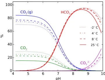
Figure 3.Partition of CO2among gas- and aqueous-phase species
under various temperatures. The calculations are conducted with 45 mL of headspace with N2 and 10 mL of solution with 10 mM
total inorganic carbon using PHREEQC. Gas phase dominates at lower pH and high temperature. As pH increases, the gas-phase CO2 fraction is very low after pH 7, implying potential underes-timation of carbon mineralization based on headspace CO2 concen-tration measurement only.
3.2.3 CO2distribution among gas, aqueous, and adsorbed phases
While increasing Fe(III) slightly increases the predicted CO2 for ridge mineral soils (Fig. 2a2), it decreases the predicted CO2 in the headspace for trough and center mineral soils (Fig. 2a1 and a3). This is because CO2 solubility is pre-dicted to increase significantly as pH increases, resulting in the dissolution of CO2from the headspace into the aqueous phase (Fig. S1 in the Supplement). To examine this impact, we conduct numerical simulations with a 45 mL headspace with an initial 1 atm N2gas and 10 mL solution with 10 mM total inorganic carbon at various temperature and pH values. CO2(g) and CO2(aq) or carbonic acid dominate at a pH lower than 5 (Fig. 3). As the pH increases above the carbonic acid pKa (around 6.3 under standard conditions), CO2(g) in the headspace and CO2(aq) decrease as HCO−3 becomes dom-inant in the aqueous phase, and the gas-phase fraction de-creases dramatically. The gas-phase fraction also dede-creases with decreasing temperatures (Fig. 3).
In addition, CO2 was reported to adsorb to surface sites (Appelo et al., 2002; van Geen et al., 1994; Villalobos and Leckie, 2000). With the surface complexation reactions between Fe(OH)3a and carbonate species, we add 1 mmol Fe(OH)3a (about the mean values in Fig. 2 for the case fFe3=0.02) to the abovementioned numerical experiments.
0
10
20
30
CO
2(%
)
(a1)
Trough
(a2)
Ridge
rganic
(a3)
Center
0
1
2
3
4
CH
4(%
)
(b1)
(b2)
(b3)
0
10
20
30
Ac (mM)
(c1)
(c2)
(c3)
0
20
40
60
80
Fe(II) (mM)
(d1)
(d2)
(d3)
flabile= 0.002
flabile
= 0.01
flabile= 0.02
0
20
40
60
Time (d)
4
5
6
7
pH
(e1)
0
20
40
60
Time (d)
(e2)
0
20
40
60
Time (d)
(e3)
O
R
Figure 4.Increasing initial labile DOC better describes the observed initial rapid CO2increase in the headspace for the organic soils. See
Fig. 2 caption for more information.
high-Fe(III) initial content cases in Fig. 2, adding CO2 sorp-tion reacsorp-tions provides a substantial buffer against the early increase in CO2in the headspace (Fig. S3). As the Fe(OH)3a is reduced and dissolved, the adsorbed CO2is predicted to be released, contributing to an increase in headspace CO2 in-crease later on.
In addition to pressure, these calculations suggest the need to appropriately account for pH and its impact on the gas, aqueous, and adsorbed phases CO2 partition when we use headspace concentration measurements from anaerobic in-cubations to estimate CO2emission. Otherwise, substantial uncertainties can be introduced. A geochemical model with accurate thermodynamic data and accounting for CO2
sorp-tion can be useful in accurately quantifying CO2production in these closed microcosms.
3.2.4 Initial CO2accumulation in the organic soil microcosms
con-tain about half total organic carbon of the other microcosms, double the water volume, and 3 to 5 times water-extractable carbon (Table 2). As a result, it produces the most CO2and CH4 and has a very short lag time between CH4and CO2. If we increase the initial labile DOC contentfLabileDOCfrom 0.0005, as shown in Fig. 2, to 0.01, and 0.02 for the organic soil microcosms, the underprediction of the early CO2 in-crease in the headspace is more or less mitigated (Fig. 4).
The predicted rapid initial CO2increase is due to the fast fermentation reactions (Fig. S4a1–6, e1–6). The predicted steep transition in CO2concentration increases appears rea-sonable for the center and trough soil microcosms, but less so for the ridge soil microcosms. In addition to the 20 h and 14-day turnover time differences, fermentation reactions crease the pH, and further inhibit the predicted SOM1 de-composition reactions, Fe(III) reduction, and methanogene-sis, making the predicted transition steeper. The fast fermen-tation is consistent with the observed rapid disappearance of glucose and increase in CO2after glucose addition in simi-lar experiments with soils from a high-center polygon trough from the same site (Yang et al., 2016). However, the observed decrease in natural free reducing sugars was gradual, with about one-third of the original reducing sugars left over af-ter 150 days of incubations. Along with the predicted rapid initial labile DOC decrease and CO2increase, the model pre-dicts a rapid initial increase in organic acids, which is close to the observations for the center soil microcosms but much greater than the observations for the trough and ridge soil mi-crocosms. The latter indicates that the ratio of organic acids to CO2of 2:1 from the fermentation Reaction (R1) may not
be accurately representative of the experiments.
Detailed measurements showed a rapid initial increase and then a quick decrease in organic acids in the mineral soil mi-crocosms and a gradual increase and slow decrease in the or-ganic soil microcosms from a trough location in a high-center polygon in the first 144 days of anaerobic incubation mineral and organic soil microcosms for ethanol, and were generally more gradual for organic acids than for ethanol (Yang et al., 2016). To explain the various observations for the organic soil microcosms and for accurate predictions, the diversity of the hydrolysis products (Feng and Simpson, 2008) and the subsequent pathways (Tveit et al., 2015) may need to be ac-counted for. Additional detailed data are needed to support increasingly mechanistic models, e.g., with reducing sugars to represent less rapid fermentation, and additional specific organic acids such as propionate and butyrate to better de-scribe diverse observations in the incubations.
3.2.5 Carbon mineralization
Less than 1 % of the total initial carbon turned over to CO2 and CH4 in about 2 months, which is attributed mostly to decomposition of labile SOM (SOM1), labile DOC, and organic acids (Fig. S4). Few changes are predicted in the slow pools (SOM3, and SOM4, not shown) even though
they comprise a large portion of the soil carbon pool. The small amount of respired carbon is similar to the incubation tests conducted with Siberian permafrost soils under 4◦C, which was estimated to be 3.1 % and 0.55 % under aero-bic and anaeroaero-bic conditions for 1200 d (Knoblauch et al., 2013), the 1-year aerobic incubation tests (Feng and Simp-son, 2008), and the incubations from a wide range of Arc-tic soils (Schädel et al., 2014). All of these results suggest that the hydrolysis of macromolecular organics by extracel-lular enzymes could be a rate-limiting step at late times. To predict the long-term vulnerability of the organic carbons, it is important to understand and describe the hydrolysis of macromolecular components in SOM.
3.2.6 CH4accumulation
Besides Fe(III) reduction, the predicted CH4 production is dependent on the substrate production. With slabile=0.2,
the model generally predicts less CH4 and more CO2than the case withslabile=0.4 because less SOM is assumed to
respire through the anaerobic pathway in theslabile=0.2 case
(Fig. S5). With increased slabile=0.6, the model predicts
more CH4 and less CO2. The impact on the mineral soils is generally more pronounced than the organic soils because the former is more substrate limiting than the latter. Unlike CO2, CH4 solubility and adsorption are much lower. Gas-phase CH4in the headspace dominates over aqueous and ad-sorbed phases. The model predicts the general exponential increase trend with a lag time behind CO2 (Fig. 2). How-ever, the prediction is sensitive to Fe(III) reduction, pH, tem-perature (Fig. 2), and labile substrates (Fig. 4). The model substantially underpredicts early fast CH4production for the center organic soil microcosms (Fig. 4b3). While the cell count for the center organic soils is not available for day 0, the data did show that the center organic soils had the highest amount of biomass after 100-day incubations (Roy Chowd-hury et al., 2015). The disagreement between the predictions and the observations can be mitigated by increasing the initial biomassfbiofrom 10−6to 10−5and 2×10⁻⁵ for the
cen-ter organic soil microcosms (Fig. 5). With increased initial biomass, Fe(III) reduction and methanogenesis are predicted to speed up the recovery of the initial pH drop caused by or-ganic acid accumulation so that the model predicts a fast CH4 increase that is comparable to the observed increase. How-ever, the model overpredicts the CH4increase at late times, indicating alternative inhibition mechanisms rather than sub-strate limitation on methanogenesis at late times or CH4 con-sumption such as anaerobic oxidation (Caldwell et al., 2008; Smemo and Yavitt, 2011).
3.2.7 pH
0 10 20 30
CO2
(%
)
(a)
0 5 10 15 20
CH4
(%
)
(b)
0 5 10 15 20 25
CO2
(m
M)
(c)
fbio = 10−6
fbio = 10−5
fbio = 2 × 10⁻⁵
05 10 15 20 25 30
Ac (mM)
(d)
0 10 20 30 40 50 60 70 Time (d)
0 5 1015 20 25 30
Fe(II) (mM)
(e)
0 20 40 60
Time (d) 4
5 6 7
pH
(f)
Figure 5.Increasing the initial biomass predicts rapid CH4
accumu-lation at early times that is close to the observations but misses the level-off trend at late times for the center organic soils. See Fig. 2 caption for more information.
evolution reasonably well (Fig. 2). The initial pH was lower in the mineral soils than in the organic soils (Fig. 2), probably because of less buffering capacity due to less organic matter in the mineral soils and/or more reducing condition in the organic soils as reduction reactions typically consume pro-tons. Because the ridge mineral soils have the lowest initial pH, the CLM4Me pH factor is the lowest (Table S1), con-tributing to the underprediction of CH4(Fig. 2b2). With high organic content, the organic matter dominates the aqueous geochemistry, and the predicted pH is sensitive to the sur-face sites specified for WHAM. If the specified WHAM or-ganic matter is reduced by 25 %, then the pH buffering capac-ity is decreased and the predicted pH increases substantially (Fig. S6e1–6) even though the predicted changes in organic acids and Fe(II) are small. For the trough soils, the predicted pH surpasses the optimal of 6.2, andf(pH) (Eq. 3) decreases (Fig. S6e1, e4). As a result, predicted CO2and CH4are de-creased. The pH impact becomes complex around the opti-mal pH. If we increase the specified WHAM organic matter by 25 %, the predicted pH is lower due to larger pH buffer-ing and the reaction rates are generally smaller. Settbuffer-ing the WHAM sites at measured total organic carbon works reason-ably well for the experiments with the CLM4Me pH response function.
Comparing the CLM4Me pH response function with these used in TEM and DLEM, all three response functions show that the reaction rates are sensitive to pH (Fig. 6), which is expected to influence the predictions for these incubation
3 4 5 6 7 8 9 10 11
pH 0.0
0.2 0.4 0.6 0.8 1.0 1.2
f(pH)
CLM4Me TEM DLEM
Figure 6.Comparison of pH response functions used in CLM4Me
(Riley et al., 2011), TEM (Raich et al., 1991), and DLEM (Tian et al., 2010) as described by Eq. (3), (A1–3). Reaction rates are sensi-tive to pH and pH response functions vary substantially, introducing prediction uncertainty.
tests as the pH increases from about 5.5 to 7. In this range, CLM4Me and DLEM have a similar slope, but the latter has a greater rate reduction effect. While CLM4Me and TEM have a similar rate reduction effect, CLM4Me has a steeper curve than TEM. These differences translate to substantial differences in model predictions (Fig. S7). All calculated f(pH) values increase during the tests (Fig. S7f1–f6). As thef(pH) calculated by DLEM is the lowest, the predicted changes are the smallest. Thef(pH) calculated by TEM is slightly greater than CLM4Me at the beginning and is the opposite at late times (Fig. 6). As a result, TEM generally predicts slightly faster evolution than CLM4Me as the reac-tion rates at the late times are limited by substrates rather than pH. While the pH ranges from 3.3 to 8.6 in the Arctic soils (Schädel et al., 2014), the range and the variability in the data are limited in the evaluation of these pH response func-tions. Nevertheless, model predictions are sensitive to pH re-sponse functions; the microbes are likely adapted to the site pH conditions such that the response functions are expected to vary among sites and functional groups. Therefore, pH re-sponse function can be an important source of prediction un-certainty.
3.2.8 Temperature response
Ar-10
-210
-110
010
1f(T)
(a)
CLM-CN
CENTURY
(b)
CLM-CN
Q10
= 1.8
Q10
= 2.0
Q10
= 2.5
20 10 0 10 20 30 40
Temperature (
◦C)
10
-210
-110
0f(T)
(c)
CLM-CN
Tm= 250 K
Tm= 260 K
Tm= 270 K
20 10 0 10 20 30 40 50
Temperature (
◦C)
(d)
CLM-CN
Ea= 50 kJ mol−1
Ea= 60 kJ mol−1
Ea= 70 kJ mol−1
Figure 7.Comparison of temperature response functions used in(a)land surface models CLM-CN (Thornton and Rosenbloom, 2005), CENTURY (Parton et al., 2010),(b)Q10(Oleson et al., 2013),(c)Ratkowsky equation (Ratkowsky et al., 1982), and(d)Arrhenius equation
(Wang et al., 2013) described by Eqs. (4, B1–B4). Reaction rates are sensitive to temperature and temperature response functions vary substantially, introducing prediction uncertainty.
rhenius equation, and Ratkowsky equation in Figs. 7 and S8. All of these temperature response functions describe in-creasing rate with inin-creasing temperature. When the tem-perature response functionsf (T )are plotted in arithmetical scale, the shapes are similar except for CENTURY, which approaches 1 when the temperature increases above 20◦C; CLM-CN is close to Q10 with Q10=2.5, the Arrhenius
equation with Ea=60 kJ mol−1 and the Ratkowsky
equa-tion with Tm=260 K. When f (T ) is plotted in log scale (Fig. 7),Q10and Arrhenius equations are approximately lin-ear, while the rest have a similar shape; CLM-CN appears close to the Ratkowsky equation with Tm=260 K. At our
temperatures −2, 4, and 8◦C, CLM-CN is very close to
CENTURY, Q10=2.5, Ea=60 kJ mol−1, and Tm=260 K
(Figs. 7, S8). Despite their consistency, the predictions can be different for the different response functions (Figs. S9, S10), reflecting the sensitivity of the temperature effect on the bio-geochemical reaction rates. The difference is amplified when different Q10, Ea, or Tm is used (not shown), introducing potentially large uncertainty in model predictions. Because the temperature response functions are expected to vary for different microorganisms, extracellular vs. intracellular en-zymes, and geochemical reactions in the soil environment, improved quantification is needed.
3.2.9 Predicted impact of headspace gas accumulation
relationships in the biogeochemical processes, the impact of headspace gas accumulation on carbon mineralization and methanogenesis is not linear. While it is debatable which ex-perimental conditions (flush the headspace or not) reflect the field conditions, biogeochemical models like ours provide a mechanistic method to account for this impact by using boundary conditions that reflect the reality. Additional tar-geted experiments and mechanistic models are necessary to better understand the impact under different conditions, and develop representations that reflect field conditions.
4 Summary and conclusion
Soil organic carbon turnover and CO2and CH4production are sensitive to redox potential and pH. However, land sur-face models typically do not explicitly simulate the redox or pH, particularly in the aqueous phase, introducing uncer-tainty in greenhouse gas predictions. To account for the im-pact of availability of electron acceptors other than O2 on soil organic matter (SOM) decomposition and methanogen-esis, we extend the CLM-CN decomposition cascade to link complex polymers with simple substrates and add Fe(III) re-duction and methanogenesis reactions. Because pH was ob-served to change substantially in the laboratory incubation tests and in the field and is a sensitive environmental variable for biogeochemical processes, we use the Windermere Hu-mic Aqueous Model (WHAM) to simulate pH buffering by SOM. To account for the speciation of CO2among gas, aque-ous, and solid (adsorbed) phases under varying pH, temper-ature, and pressure values, as well as the impact on typically measured headspace concentration, we use a geochemical model and an established reaction database to describe obser-vations in recent anaerobic microcosms. Our results demon-strate the efficacy of using geochemical models to mechanis-tically represent the soil biogeochemical processes for Earth system models.
Together with the speciation reactions from the established geochemical database and surface complexation reactions for ferric hydrous oxides, WHAM enables us to approximately buffer an initial pH drop due to organic acid accumulation caused by fermentation and then a pH increase due to Fe(III) reduction and methanogenesis. The single input parameter for WHAM is total organic carbon content, which is avail-able in any SOM decomposition model. Therefore, adding WHAM does not necessitate any additional characterization. However, the temperature effects on surface complexation reactions with ferric hydrous oxides and organic matter may need to be further quantified.
The equilibrium geochemical speciation reactions predict a substantial increase in CO2 solubility as the pH increases above 6.3 because the aqueous dominant species shifts from CO2 to HCO−3. Adding CO2adsorption to surface sites of metal oxides further increases predicted solubility at low pH. Without taking speciation, pH, and the temperature and
pres-sure impact into consideration, the carbon mineralization rate can be substantially underestimated from anaerobic micro-cosms based on headspace CO2measurements.
Because various microbes respond to the temperature and pH change differently, it is challenging to describe observed diverse responses with any single one of the existing re-sponse functions. As the microbes adapt to the low temper-ature and pH conditions in the Arctic, the optimal growth temperature and pH value in these response functions may need to be adjusted to account for biological acclimation.
We demonstrate that a geochemical model can mechanis-tically predict pH evolution and accounts for the impact of pH on biogeochemical reactions, which enhances our under-standing of and ability to quantify the experimental observa-tions. Because pH is an important environmental variable in the ecosystems and land surface models either specify a fixed pH or use simple empirical equations, a geochemical model has the potential to improve model predictability for green-house emissions by mechanistically representing the soil bio-geochemical processes.
Another follow-up task could be assessing this new frame-work of anaerobic SOM decomposition in field studies with CLM-PFLOTRAN. This can be done incrementally, i.e., adding/removing reactions one at a time without source code modifications. CLM-PFLOTRAN currently uses the CLM4.5 vertically resolved grid. The resolution can be ad-justed, possibly in three dimensions, to reflect the hetero-geneity of any structural soil column to account for the limi-tation of electron donors and electron acceptors at individual locations. As we gradually implement more and more pro-cesses, such as gas and aqueous transport through soils and aerenchyma, explicitly representing microbial processes for carbon decomposition, we hope the new framework will be useful for future investigation and model developments.
5 Code availability
PHREEQC is publicly available at http://wwwbrr.cr.usgs. gov/projects/GWC_coupled/phreeqc/.
6 Data availability
Appendix A: Additional pH response functions
With pHmin, pHopt, and pHmaxof 4, 7, and 10 with no mi-crobial activity at pH below pHmin or above pHmax, the pH response function used in DLEM is (Tian et al., 2010)
f (pH)= 1.02
1.02+106exp(−2.5 pH), (A1)
for pH < 7; otherwise,
f (pH)= 1.02
1.02+106exp(−2.5(14−pH)). (A2)
TEM uses a bell-shaped function (Cao et al., 1995; Xu et al., 2015; Raich et al., 1991)
f (pH)= (pH−pHmin)(pH−pHmax) (pH−pHmin)(pH−pHmax)−
pH−pHopt
pHopt, (A3)
with pHmin, pHopt, and pHmax=5.5, 7.5, and 9, respectively
(Cao et al., 1995). Considering the typical acidic conditions in the Arctic and wetlands, we use the DLEM parameter val-ues (Tian et al., 2010) as substantial CH4was observed in the incubation tests below pH 5.5 (Roy Chowdhury et al., 2015).
Appendix B: Additional temperature response functions
TheQ10method is the most common temperature response function used in LSMs (Xu et al., 2016b; Berrittella and Van Huissteden, 2009, 2011; Walter and Heimann, 2000; Zhuang et al., 2004; Riley et al., 2011; Oleson et al., 2013). It is
f (T )=Q T−Tref
10
10 , (B1)
withTrefas a reference temperature usually at 25◦C. How-ever, the Q10 value varies from 1.5 to 28 (Segers, 1998; Mikan et al., 2002), which indicates inadequate represen-tation of the supply of substrates (Davidson and Janssens, 2006; Davidson et al., 2006), and microbial functional groups (Blake et al., 2015; Svensson, 1984; Rivkina et al., 2007; Lu et al., 2015) and necessitates alternative tempera-ture response functions.
The Arrhenius equation (Arah and Stephen, 1998; Wang et al., 2012; Grant, 1998; Grant et al., 1993; Sharpe and DeMichele, 1977; Grant and Roulet, 2002) is
f (T )=exp
−Ea
R
1
T − 1 Tref
, (B2)
withEaas the activation energy andRas the gas constant. It is related to theQ10method with ln(Q10)= 10Ea
RTrefT. The in-troduced variability by the absolute temperatureT is not able to explain the wide range ofQ10values either. Consequently, empirical equations are often used (Nicolardot et al., 1994). DayCent, ForCent, and CENTURY use (Parton et al., 2010) f (T )=0.56+0.465a tan [0.097(T−15.7)]. (B3)
A temperature response function for microbial growth is (Ratkowsky et al., 1982)
f (T )=
T
−Tm Tref−Tm
2
, (B4)
The Supplement related to this article is available online at doi:10.5194/bg-13-5021-2016-supplement.
Disclaimer. This manuscript has been authored by UT-Battelle, LLC, under contract no. DE-AC05-00OR22725 with the US De-partment of Energy. The publisher, by accepting the article for pub-lication, acknowledges that the United States Government retains a non-exclusive, paid-up, irrevocable, worldwide license to publish or reproduce the published form of this manuscript, or allow others to do so, for United States Government purposes. The Department of Energy will provide public access to these results of federally sponsored research in accordance with the DOE Public Access Plan (http://energy.gov/downloads/doe-public-access-plan).
Acknowledgements. This research was funded by the US Depart-ment of Energy, Office of Sciences, Biological and EnvironDepart-mental Research, Terrestrial Ecosystem Sciences Program, and is a product of the Next-Generation Ecosystem Experiments in the Arctic (NGEE-Arctic) project. ORNL is managed by UT-Battelle, LLC, for the US Department of Energy under contract DE-AC05-00OR22725. Xiaofeng Xu is grateful for the support from the San Diego State University.
Edited by: T. Keenan
Reviewed by: three anonymous referees
References
Abbott, B. W., Larouche, J. R., Jones, J. B., Bowden, W. B., and Balser, A. W.: Elevated dissolved organic carbon biodegradabil-ity from thawing and collapsing permafrost, J. Geophys. Res.-Biogeo., 119, 2049–2063, doi:10.1002/2014JG002678, 2014. Appelo, C. A. J., Van Der Weiden, M. J. J., Tournassat, C., and
Charlet, L.: Surface Complexation of Ferrous Iron and Carbonate on Ferrihydrite and the Mobilization of Arsenic, Environ. Sci. Technol., 36, 3096–3103, doi:10.1021/es010130n, 2002. Arah, J. R. M. and Stephen, K. D.: A model of the processes leading
to methane emission from peatland, Atmos. Environ., 32, 3257– 3264, doi:10.1016/S1352-2310(98)00052-1, 1998.
Arnosti, C.: Rapid potential rates of extracellular enzymatic hy-drolysis in Arctic sediments, Limnol. Oceanogr., 43, 315–324, doi:10.4319/lo.1998.43.2.0315, 1998.
Arnosti, C.: Substrate specificity in polysaccharide hydrolysis: Con-trasts between bottom water and sediments, Limnol. Oceanogr., 45, 1112–1119, doi:10.4319/lo.2000.45.5.1112, 2000.
Arnosti, C., Jørgensen, B. B., Sagemann, J., and Thamdrup, B.: Temperature dependence of microbial degradation of organic matter in marine sediments: polysaccharide hydrolysis, oxygen consumption, and sulfate reduction, Mar. Ecol.-Prog. Ser., 165, 59–70, doi:10.3354/meps165059, 1998.
Berrittella, C. and Van Huissteden, J.: Uncertainties in modelling CH4 emissions from northern wetlands in glacial climates: effect of hydrological model and CH4model structure, Clim. Past, 5,
361–373, doi:10.5194/cp-5-361-2009, 2009.
Berrittella, C. and van Huissteden, J.: Uncertainties in modelling CH4 emissions from northern wetlands in glacial climates: the role of vegetation parameters, Clim. Past, 7, 1075–1087, doi:10.1021/es010130n, 2011.
Bethke, C. M., Sanford, R. A., Kirk, M. F., Jin, Q., and Flynn, T. M.: The thermodynamic ladder in geomicrobiology, Am. J. Sci., 311, 183–210, doi:10.2475/03.2011.01, 2011.
Blake, L. I., Tveit, A., Øvreås, L., Head, I. M., and Gray, N. D.: Re-sponse of Methanogens in Arctic Sediments to Temperature and Methanogenic Substrate Availability, PLoS ONE, 10, e0129733, doi:10.1371/journal.pone.0129733, 2015.
Bockheim, J. G., Hinkel, K. M., and Nelson, F. E.: Soils of the Barrow region, Alaska, Polar Geography, 25, 163–181, doi:10.1080/10889370109377711, 2001.
Bridgham, S. D., Cadillo-Quiroz, H., Keller, J. K., and Zhuang, Q.: Methane emissions from wetlands: biogeochemical, micro-bial, and modeling perspectives from local to global scales, Glob. Change Biol., 19, 1325–1346, doi:10.1111/gcb.12131, 2013. Caldwell, S. L., Laidler, J. R., Brewer, E. A., Eberly, J. O.,
Sandborgh, S. C., and Colwell, F. S.: Anaerobic Oxidation of Methane: Mechanisms, Bioenergetics, and the Ecology of Asso-ciated Microorganisms, Environ. Sci. Technol., 42, 6791–6799, doi:10.1021/es800120b, 2008.
Cao, M., Dent, J. B., and Heal, O. W.: Modeling methane emis-sions from rice paddies, Global Biogeochem. Cy., 9, 183–195, doi:10.1029/94GB03231, 1995.
Cao, M., Gregson, K., and Marshall, S.: Global methane emis-sion from wetlands and its sensitivity to climate change, Atmos. Environ., 32, 3293–3299, doi:10.1016/S1352-2310(98)00105-8, 1998.
Cheng, K., Ogle, S. M., Parton, W. J., and Pan, G.: Pre-dicting methanogenesis from rice paddies using the DAY-CENT ecosystem model, Ecol. Modell., 261/262, 19–31, doi:10.1016/j.ecolmodel.2013.04.003, 2013.
Conrad, R.: Soil microorganisms as controllers of atmospheric trace gases (H2, CO, CH4, OCS, N2O, and NO), Microbiol. Rev., 60, 609–640, 1996.
Cui, M., Ma, A., Qi, H., Zhuang, X., Zhuang, G., and Zhao, G.: Warmer temperature accelerates methane emissions from the Zoige wetland on the Tibetan Plateau without changing methanogenic community composition, Scientific Reports, 5, 11616, doi:10.1038/srep11616, 2015.
Davidson, E. A. and Janssens, I. A.: Temperature sensitivity of soil carbon decomposition and feedbacks to climate change, Nature, 440, 165–173, doi:10.1038/nature04514, 2006.
Davidson, E. A., Janssens, I. A., and Luo, Y.: On the vari-ability of respiration in terrestrial ecosystems: moving beyond Q10, Glob. Change Biol., 12, 154–164, doi:10.1111/j.1365-2486.2005.01065.x, 2006.
Drake, H. L., Horn, M. A., and Wüst, P. K.: Intermediary ecosystem metabolism as a main driver of methanogenesis in acidic wetland soil, Environ. Microbiol. Reports, 1, 307–318, doi:10.1111/j.1758-2229.2009.00050.x, 2009.