Lat. Am. j. solids struct. vol.11 número10

(1)

Abstract

An efficient piezoelectric sandwich beam finite element is present-ed here. It employs the couplpresent-ed polynomial field interpolation scheme for field variables which incorporates electromechanical coupling at interpolation level itself; unlike conventional sandwich beam theory (SBT) based formulations available in the literature. A variational formulation is used to derive the governing equa-tions, which are used to establish the relationships between field variables. These relations lead to the coupled polynomial field descriptions of variables, unlike conventional SBT formulations which use assumed independent polynomials. The relative axial displacement is expressed only by coupled terms containing con-tributions from other mechanical and electrical variables, thus eliminating use of the transverse displacement derivative as a degree of freedom. A set of coupled shape function based on these polynomials has shown the improvement in the convergence char-acteristics of the SBT based formulation. This improvement in the performance is achieved with one nodal degree of freedom lesser than the conventional SBT formulations.

Keywords

Coupled field, finite elements, sandwich beam, piezoelectric, smart structure, shear mode.

An efficient coupled polynomial interpolation scheme

for shear mode sandwich beam finite element

1 INTRODUCTION

Piezoelectric smart structures are vital part of today's structural and vibration control technology (Crawley and de Luis, 1987; Sulbhewar and Raveendranath, 2014b). Piezoelectric materials have coupling between electrical and mechanical fields which determines the response of the system. The piezoelectric material can be used in two modes of operation depending on the kind of elec-tromechanical coupling present. Either the piezoelectric material can be surface bonded to the host structure or sandwiched between host layers. The surface bonded extension mode model is based on coupling between the longitudinal motion of transversely poled piezoelectric material

Litesh N . Sulbhewar a P. Raveendranath b

Department of Aerospace Enginee-ring, Indian Institute of Space Science and Techology, Thiruvananthapuram, India.

a_{(Corresponding author) Research}

Scholar

Email: [email protected]

b _Adjunct_Professor

(2)

Latin American Journal of Solids and Structures 11 (2014) 1864-1885

and the transverse electric field. While in sandwich shear mode model, coupling between shear deformation of axially poled piezoelectric material and the transverse electric field is used (Ben-jeddou et al., 1997; Zhang and Sun, 1996).

The advantages of shear mode sandwich beams over surface mounted extension mode beams were first reported by Sun and Zhang (1995). They proved the merits of shear mode beam over the conventional extension mode beam by comparative study with 2D finite element simulation using ANSYS software. They also mentioned that shear mode beams are more suitable for high-frequency amplitude cases, while extension mode surface mounted beams are suitable for low-frequency high-amplitude cases.

Surface mounted actuators in the extension mode beams are placed at the extreme thickness positions of the host structure, thus actuator might be subjected to high bending stresses (Sun and Zhang, 1995; Abramovich, 2003). The adaptive sandwich shear mode beam has the ad-vantage of lower stresses in the actuator and along the interface between the actuator and the host structure. This minimizes debonding problems and is known to contribute to the structural integrity of the actuator (Benjeddou et al., 1997).

Many researchers have provided analytical solutions using various theories to describe the be-haviour of shear mode sandwich structures. Vel and Batra (2001) proposed an exact 3D state space solution for the static cylindrical bending of simply supported laminated plates with em-bedded shear mode piezoelectric layers. Zhang and Sun (1996) used the classical sandwich beam theory (SBT) to give an analytical model for shear mode beams in which, conventional material faces are modeled by Euler-Bernoulli beam and the piezoelectric core by First-order Shear Defor-mation Theory (FSDT). Zhang and Sun (1999) presented analytical solutions for a sandwich plate with a piezoelectric core using the principle of minimum potential energy and Raleigh-Ritz method. They validated the analytical solutions with finite element simulations. Abramovich (2003) and Edery-Azulay and Abramovich (2004) proposed FSDT based closed form solutions for bending angle and axial and lateral displacements for shear mode smart beams and carried out a parametric study for various configurations, lay-ups and boundary conditions. Analytical solu-tions using the state-space approach along with the Jordan canonical form were proposed by Al-draihem and Khdeir (2000; 2003) to solve beam bending problem for beams with continuous and segmented piezoelectric actuators, respectively. They provided both FSDT and HSDT (Higher-order Shear Deformation Theory) based solutions. By numerical experiments, they showed that FSDT based solutions are very sensitive to shear correction factor and has pronounced difference with HSDT solutions. Khdeir and Aldraihem (2001) extended this formulation with discontinuity function to perform the parametric study of shear actuated beams. Aldraihem and Khdeir (2006; 2012) proposed analytical solutions for bending deformations of antisymmetric angle ply laminat-ed plates with thickness shear piezoelectric actuators baslaminat-ed on FSDT and HSDT, respectively using L`evy method, in conjunction with the state-space approach. Poizat and Benjeddou (2006) presented analytical formulae for shear monomorphs which were validated by 3D finite element simulation using commercial package.

(3)

Baillargeon and Vel (2005) carried out an experimental and numerical assessment of vibration suppression of smart structure using shear mode piezoelectric actuators. The results obtained were validated by comparison with 2D finite element simulations using ABAQUS software.

Many researchers have reported different finite element formulations for shear mode sandwich beam. FSDT based beam finite element was proposed by Rathi and Khan (2012) to study vibra-tion attenuavibra-tion and shape control of smart beams. Beheshti-Aval et al. (2013) developed a cou-pled refined high-order global-local theory for static analysis of shear mode piezoelectric sandwich composite beams. Kapuria and Hagedorn (2007) proposed a unified layerwise theory for piezoelec-tric smart beams and validated their formulation with finite element simulations using ABAQUS. The SBT has been favored by many researchers to formulate sandwich beam finite elements. Benjeddou et al. (1997; 2000) presented a unified finite element model for analysis of smart beams in both extension and shear mode, based on SBT. A parametric study carried out by Benjeddou et al. (2000) showed that the shear actuation mechanism has several promising features over con-ventional extension mode beams for stiff structures with thick piezoelectric layers. Benjeddou et al. (1999) developed a SBT based finite element with improved kinematics to remove shear lock-ing present in their earlier work (Benjeddou, 1997). Raja et al. (2002) used a generalized SBT by considering laminates (instead of single layer) for the faces, for dynamic analysis of smart beams. They showed that in active vibration control, shear mode beams are more effective than the con-ventional extension mode beams, for the same control effort. Trindade and Benjeddou (2006; 2008) used a modified SBT with Third-order Shear Deformation Theory (TSDT) for core and Euler-Bernoulli beam theory for faces to investigate the effect of the induced potential on the structural behaviour of sandwich beams.

All SBT-based finite element models available in the literature have used assumed independ-ent polynomials for interpolation of electric potindepend-ential and mechanical field variables. These inde-pendent polynomial based formulations show slower convergence. An efficient way to improve performance of finite elements is the use of coupled polynomials (Raveendranath et al., 1999; 2000). Recently, Sulbhewar and Raveendranath (2014a) proposed a coupled polynomial field in-terpolation scheme to improve convergence of HSDT based extension mode piezoelectric beam finite elements.

In the present work, we introduce coupled polynomial expressions derived from governing equations, for interpolation of the field variables. Relative axial displacement of beam faces (u!) is expressed by a purely coupled polynomial having contributions from mid-plane transverse dis-placement (w0) and relative electric potential (!!) without any independent terms. As proved by the numerical experiments, the present coupled polynomial field SBT formulation gives better convergence of finite element results than the conventional independent polynomial field SBT formulations for static (both actuator and sensor configurations) and modal analyses. All conven-tional SBT formulations have four mechanical degrees of freedom per node while the present for-mulation requires only three, owing to a coupled polynomial interpolation scheme which interpo-lates relative axial displacement of beam faces (u!) purely by coupled terms. The accuracy and

(4)

2 THEORETICAL FORMULATION

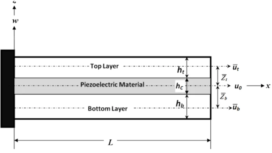
Consider a three layered beam with piezoelectric core sandwiched between face layers as shown in Figure 1. The face layers can be of conventional homogeneous material or laminates of composite material. The beam layers are assumed to be of isotropic or specially orthotropic materials with perfect bonding between them. Faces of piezoelectric layers are assumed to be fully covered with electrodes. The mathematical model is based on sandwich beam theory (SBT) with layerwise electrical potential which follows linear theories of elasticity and piezoelectricity.

Figure 1: Geometry of a general shear mode piezoelectric sandwich beam.

2.1 Mechanical Displacements and Strains

The improved kinematic field for SBT given by Benjeddou et al. (1999) is used here for further formulation:

u

i(x,z)= u(x)± ! u₍x₎

2

! "

# $

% & ' z_'z

i

(

)

w

0

'₍_x_), _i ₌_t₍₊_),_b₍_'₎

u

c(x,z)= u(x)+dw0 '₍_x₎

(

)

+_z u!(x)

h

c

+!w 0

'₍_x₎ !

"

## $

% &&

(1)

where d =(h

t!hb

) / 4and != h t+hb

(

)

/ (2h

c). uand u!are the mean and relative axial

displace-ments of upper and lower sandwich beam faces, defined as u =(u

t+ub) / 2and u!=ut!ub, respec-tively. u

tand ubare the mid-plane displacements of upper and lower surface layers. ( ) 'denotes

derivative with respect to x. L B h_{, ,}

are the length, width and the total thickness of the beam, respectively. The indices t b c, ,

denote the top, bottom and core layers of the sandwich beam, respectively.

The transverse deflection is taken as constant throughout the thickness given as:

w₍x_,z₎=w

0(x)

(5)

Mechanical axial and shear strain fields are derived using usual strain-displacement relations as:

!x i

(x_,z₎=!ui(x,z) !x =

u'₍x₎±u! '₍_x₎

2 " # $ $ % & '

' (

(

z(zi

)

w₀

''₍_x_), _i ₌_t₍₊_),_b₍₍₎

!_xc(x_,z₎=!uc(x,z) !x =

u'₍x₎+dw

0 ''

(x₎

(

)

+_z u!

'₍_x₎ h

c

+!w

0 ''

(x₎

" # $ $ % & ' ' (3) !xz c

(x_,z₎=!uc(x,z) !z +

!w₍x_,z₎ !x =

!

u₍x₎

h c

+(!+1)w

0 '₍_x₎

"

#

$$ %

&

'' (4)

2.2 Electric Potential and Electric Field

The through-thickness profile of the electric potential !(x_,_z₎in piezoelectric core is taken as

line-ar as used by Benjeddou et al. (1997; 1999; 2000). The electric field in transverse direction _E_zcan be derived from electric potential as (Benjeddou et al., 1999):

E

z(x,z)=!

"!(x_,z₎

"z =!

!

!(x₎ h

c

(5)

where _!!is the difference of potentials at the top and bottom faces of piezoelectric core.

3 REDUCED CONSTITUTIVE RELATIONS

The piezoelectric material with orthotropic properties is considered here. It has axes of material symmetry parallel to beam axes, in which electric field is applied in the transverse direction. For shear mode beams, axially poled piezoelectric material layer is subjected to the transverse electric field. The elastic, piezoelectric and dielectric constants are denoted by

C

ij

,

e

kj

(i

,

j

=

1...6)

and

!k(k =1,2,3), respectively. The transformed coupled constitutive equations for axially poled

piezo-electric material are given as (Benjeddou et al. 1997):

!x !_y ! z !_yz !xz !_xy D_x D_y D_z ! " # # # # # # # # # # # # # # $ % & & & & & & & & & & & & & & =

C33 C23 C13 0 0 0 'e33 0 0

C23 C22 C12 0 0 0 'e32 0 0

C13 C12 C11 0 0 0 'e31 0 0

0 0 0 _C

66 0 0 0 0 0

0 0 0 0 _C

55 0 0 0 'e15

0 0 0 0 0 _C

44 0 'e24 0

e33 e32 e31 0 0 0 (3 0 0

0 0 0 0 0 _e

24 0 (2 0

0 0 0 0 _e

15 0 0 0 (1

! " # # # # # # # # # # # # # # # # # # # # # # # # # # # # $ % & & & & & & & & & & & & & & & & & & & & & & & & & & & & !x !_y ! z !_yz !xz !xy

(6)

where !,!,!,!,_Dand _Edenote normal stress (N/m2), shear stress (N/m2), normal strain, shear strain, electric displacement (C/m2) and electric field (V/m), respectively.

_y=0_{(Sulbhewar and}

Raveendranath, 2014a). Only the coupling between shear deformation and transverse electric field is effective for shear mode beams. Using these conditions in constitutive equation (6), we get:

!_x

!_x_z

D_z !

" # # #

$

% & & &=

!

Q11 0 0

0 _Q!

55 'e!15

0 e!

15 ! (1 !

" # # # # #

$

% & & & & &

!_x

!xz

E

z

!

" # # #

$

% & & &

(7)

where _Q!

11=Q33! Q23 2 _Q

22

(

)

, Q_ij =C_ij! C1iC1j C₁₁ "

# $ $

%

& '

'(i,j =2,3);Q!55=C55,e!15=e15, ! !₁=!₁.

4 VARIATIONAL FORMULATION

Hamilton’s principle is used to formulate piezoelectric smart beam. It is expressed as (Sulbhewar and Raveendranath, 2014a):

! (K _!H ₊W₎dt₌

t

1

t

2

"

(!_K !!_H +!W₎dt₌₀

t

1

t

2

"

(8)

where, K=kinetic energy, H =electric enthalpy density function for piezoelectric material and me-chanical strain energy for the linear elastic material and W =external work done.

4.1 Electromechanical and Strain Energy Variations

For faces made of conventional/composite materials, the mechanical strain energy variation is given as:

(

i i

)

,

i x x V

H dV i b t

δ =

_∫

σ δε = (9)

The electromechanical strain energy variation of piezoelectric core is given as:

(

c c c c c c

)

c x x xz xz z z

V

H D E dV

δ =

_∫

σ δε +τ δγ − δ (10)

(7)

Latin American Journal of Solids and Structures 11 (2014) 1864-1885 !H t 1 t 2

!

dt=

!

Q₁₁bI₀b+Q!₁₁cI

0 c

+Q!₁₁tI₀t

"

# $%u'+ &Q!11 b

I₀b/ 2+Q!₁₁cI₁c/h_c+Q!₁₁tI₀t / 2

"

# $%u!'+

&Q!₁₁b

(

I₁b&I₀bz_b

)

+Q!₁₁c I 0 c_d +I 1 c !

(

)

&Q!₁₁t

(

I₁t&I₀tz_t

)

" #'

$ %(w0

'' ) * + + + , -. . .

!u' / 0 1 2 1 x

!

+ t 1 t 2

!

&_Q! 11

b

I

0 / 2+Q!11 c

I₁c/h_c+Q!₁₁t I

0 t

/ 2

"

# $%u

'₊ _Q!

11 b

I₀b / 4+Q!₁₁cI₂c/h c

2₊_Q!

11

t

I₀t / 4

"

# $%u!'+

!

Q₁₁b

(

I₁b&I₀bz_b

)

/ 2+Q!₁₁c I₁cd /h_c+I₂c!/h c

(

)

&_Q!

11 I 1 &I 0 z

(

)

/ 2

" #'

$ %(w0

)

"

#' $%(u'

+ Q!₁₁b

(

I₁b&I₀bz_b

)

/ 2+Q!₁₁c I₁cd /h_c+I₂c!/h c

(

)

&_Q!

11 t _I

1 t_&_I

0 t_z

t

(

)

/ 2

"

#' $%(u!'+

!

Q₁₁b

(

I₂b&2I₁bz_b+I₀bz_b2

)

+Q! 11 c I 0 c 2₊₂

I 1

c

!d +I

2 c !2

(

)

+! 11 t 2 t &2 1 t t+ 0 t t 2

(

)

"

#' $%(w0

'' ) * + + + + + + , -. . . . . . !w 0 ''₊ ! Q₅₅cI

0

c

/h

c

2

(

)

u!+ Q!₅₅cI

0 c

(!+1) /h c

"

# $%w0

'₊ _! e

15I0

c /h

c 2

(

)

_!!

(

)

!u!+

!

Q₅₅cI₀c(!+1) /h c "

# $%u!+ Q!55 c_I

0 c_(!₊

1)2

"

# $%w0

'₊ _e_! 15I0

c

(!+1) /h c

(

)

_!!

(

)

!w

0 '₊

!

e

)

_!!

(

)

!_!!

}

xt

(11)

where for th

k layer

_I

q

k

=

B

z

k+1

q+1

!

z

_kq+1

q

+1 (

k

=

b

,

c

,

t

) . b

z and z_tare the distances of the top and

bottom layer mid-surfaces from beam centerline.

4.2 Variation of Kinetic Energy

Total kinetic energy of the beam is given as (Sulbhewar and Raveendranath, 2014a):

K

₌1

2

b

_!

k z k z_k +1

!

x

!

(

u

!2₊

w

!2

)

dz dx

(12)

(8)

Latin American Journal of Solids and Structures 11 (2014) 1864-1885 !K t 1 t 2

!

dt="

!_bI 0

b

+!_cI 0

c +!_tI

0

t #

$ %&u!!+ "!bI0 b

/+! cI1

c /h

c+!tI0

t / #

$ %&u""!+

"!_b I 1 b "I 0 b zb

!

t 1 t 2

!

"!bI0 b

/+! cI1

c /h

c+!tI₀ t

/ #

$ %&u!!+ !bI0

b /4+!

cI2

c

/ 2

# $'

% &(w!!0

' ) * + + + , -. . .

!u!+

"!_b I1 b_"

I0 b_z

b

(

)

+!_c I0 c_d₊_I

1 c_!

(

)

"!t I1

&(!w0

}

dxdt

(13)

where ( ) .

denotes ! !t.

4.3 Variation of Work of External Forces

Total virtual work of the structure can be defined as product of virtual displacements with forces for the mechanical work and the product of the virtual electric potential with the charges for the electrical work. The variation of total work done by external mechanical and electrical loading is given by (Sulbhewar and Raveendranath, 2014a):

!W dt=

t₁ t

2

!

!u_f u

V ₊

!w_f w

V

(

)

dV +

(

!uf_uS +!wf_wS

)

dS S

!

V

!

+

!uf_uC +!wf_wC

(

)

" !"q0dS!

S !

!

#

$ % & & ' & & ( ) & & * & & t₁ t 2

!

dt (14)

in which fV,f S,f C are volume, surface and point forces, respectively. q0and S! are the charge density and area on which charge is applied.

5 DERIVATION OF COUPLED FIELD RELATIONS

The relationship between field variables is established here using static governing equations. For static conditions without any external loading, the variational principle given in equation (8) reduc-es to (Sulbhewar and Raveendranath, 2014a):

0 H

δ = (15)

(9)

Latin American Journal of Solids and Structures 11 (2014) 1864-1885 !u:

! Q11 b I 0 b

+Q!11 c

I0 c₊_Q!

11

t

I0

t

!

" #$u

'' + %_Q!

11 b

I0 b _{/ 2}₊_Q!

11 c

I1 c_/

h_c+Q!11

t I0

t

/ 2 !

" #$u!

!

"& #$'w0

''' ( ) * * * + ,

-=0 (16)

!u!_:

! !_Q! 11

b_I 0

b

/ 2+Q!₁₁cI₁c/h_c+Q!₁₁ I 0 / 2 " # $%

''_! _Q! 11

b_I 0

b

/ 4+Q!₁₁cI

2

c

/h c

2₊_Q! 11

t

I₀t/ 4 "

# $%u!''!

!

Q₁₁b I

1 b !I 0 b_z b

(

)

/ 2+Q!₁₁c I₁cd /h_c+I₂c!/h c

(

)

!_Q!

11 t _I

1 t_!_I

0 t_z

t

(

)

/ 2

)

!Q!₁₁t

(

I₁t!I₀tz_t

)

" #

$ %_&'u'''

+ Q!₁₁b I

1 b !I 0 b z b

(

)

/ 2+Q!₁₁c I₁cd /h_c+I₂c!/

c

(

)

!_Q!

11

t

I₁t!I₀tz_t

(

)

/ 2

"

#$ %&'u!

'''₊ ! Q₁₁ I 2

! _Q! 55

c

I₀c(!+1) /h c

"

# %&u!'! Q!55 c_I

0 c₍_!₊₁₎2 "

# %&w0 ''_! _e_!

15I0

c

(!+1) /h c

(

)

_!!' ( ) * * * * * * * * + ,

-=0 (18)

The equations (16)-(18) can be written in a simplified form as:

!u:A

1 u_u''

+A

2 u

! u''₊A

3 u_w

0 '''

=0 (19)

!u!:_!A 1

u u''_!A

2 u

!

u''_!A 3 u w 0 ''' +A 4 u ! u₊A

5 u w 0 ' +A 6 u !

!=0 (20)

!w0:A1 w_u'''

+A

2 w

!

u'''₊A

3 w_w 0 '''' !A 4 w ! u'_!A

5 w_w 0 '' !A 6 w_!

!'=0 (21)

From equation (21), neglecting higher-order terms, we get:

!

u''=! A5

w

A₄w

" # $ $ % & ' 'w0

''' ! A6

w

A₄w

" # $ $ % & ' '!! '' (22)

Using equation (22) in (19), the relationship of mean axial displacement uwith transverse

dis-placement w0and electric potential ϕis written as:

u''=!

1 m

w

0

+!₂m_!!'' (23)

where !₁m=A2 u

A

1 u

A₅w

A

4 w !

A₃u

A

1

u and !

m =A u A 1 u A 6 w A 4 w .

Using equations (22) and (23) in equation (20), the relative axial displacement can be expressed in terms of transverse displacement w0and electric potential ϕas:

!

u₌_!

1

r w

0 '

+!₂r w

0 '''

+!3r!!+"4r!! ''

(10)

where !₁r =!A5

u

A

4

u;!2

r

=A1

u

A

4

u

A

2

u

A

1

u

A

5

w

A

4

w !

A

3

u

A

1

u

"

# $ $

%

& ' '+

A

3

u

A

4

u !

A

2

u

A

4

u

A

5

w

A

4

w;!3 r

=!A6

u

A

4

u and !4

r

=A1

u

A 4

u

A₂u

A 1

u

A₆w

A 4

w!

A₂u

A 4

u

A₆w

A 4

w .

From equations (23) and (24) it is clear that the coupling constants !_im(i ₌_1,2)and _!

j r

(j =1,2,3,4)

depend only on material and geometric properties of the beam. They relate all field variables by properly accommodating all couplings in a variationally consistent manner. These relations are used in the next section to derive coupled polynomials for field variables.

6 FINITE ELEMENT FORMULATION

Using the variational formulation described above, the finite element model is developed here. For finite element formulation, the degrees of freedom consist of three mechanical (u,u!,w

0) and an elec-trical (_!!₎variables. In terms of natural coordinate_ξ, a cubic polynomial is assumed for w₀and a

linear polynomial for _!! as given in equations (25a) and (25b), respectively. The transformation

between the coordinate !and global coordinate xis given as !=[2(x!x

1) / (x2!x1)]!1with

2 1

(x −x)=l, being the length of the beam element.

w

0=b0+b1!+b2! 2

+b

3!

3 (25a)

! !=c₀+c

1" (25b)

Using these polynomials for w0and !!in equation (23) and integrating with respect toξ, we get the

coupled polynomial expression for mean axial displacement uas:

u =

(

(6!₁m/l)!2

)

b

3+a1!+a0

(26)

Substituting equations (25a) and (25b) in (24), the coupled polynomial for relative axial displace-ment u! is obtained as:

! u₌ _!

1

r₍

/l)

(

)

b

1+ 2!1

r_{(2 /}_l₎_!

(

)

b

2+ 3!1

r₍

/l)! 2₊₆_!

2 r_{(2 /}_l₎3

(

)

b

3+ !3 r

( )

c 0

+(!3

r_!₎_c

1

(27)

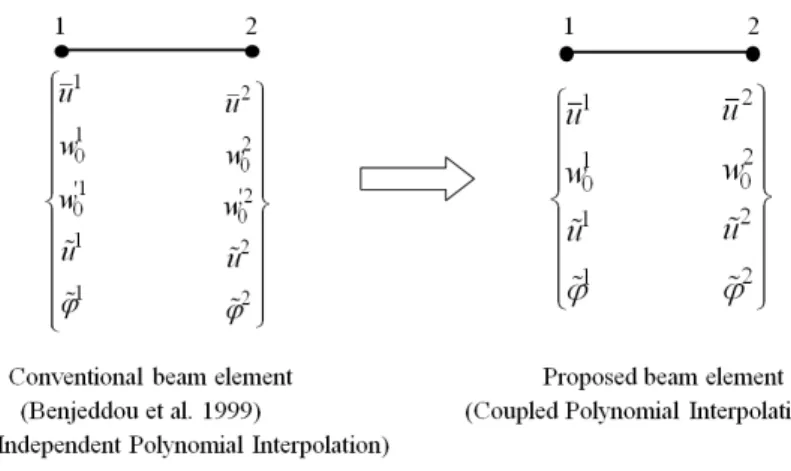
Equation (27) interpolates the relative axial displacement u!by purely coupled terms and no inde-pendent terms are present in it. The above set of interpolation polynomials consists of a total 8 generalized degrees of freedom, which is consistent with the total number of nodal degrees of free-dom for the element. Figure 2 shows the comparison of nodal degrees of freefree-dom for the present SBT based element and SBT based element of Benjeddou et al. (1999). It may be noted that the use of '

0

(11)

Figure 2: Comparison of conventional and proposed beam elements.

Using the above polynomial expressions, the coupled shape functions N

i u

!

" #$, N

i u

! " #$, N

i w

!

" #$and Ni !

! " #$in equation (28) are derived by usual method.

u w 0 ! u ! ! ! " # # $ # # % & # # ' # # = N 1 u 0 0 0 N 2 u N 1 u N 1 w 0

N₃u

N

3 u

N₂w

0

N

4 u

N₃u

N₃w

N

1 !

N₅u

0

N₆u

N

4 u

N₄w

0

N₇u

N

5 u

N₅w

0

N

8 u

N₆u

N

6 w

N₂!

( ) * * * * * * * + , -u1

w₀1

! u1 ! !1 u2 w 0 2 ! u2 ! !2 ! " # # # # # # $ # # # # # # % & # # # # # # ' # # # # # # (28)

The polynomial expressions for these shape functions in natural coordinate system are:

N

1

u =1!!

2 ;

N

2

u

= 3!1

m

!₁rl

2!₁r

l2+24!₂r(!

2_!

1); N 3

u

= 3!1

m l2

4!₁r_l2₊

48!₂r (! 2_!

1);

4 u

= 3!1

m

!₃rl2

4!₁r_l2₊

48!₂r (1!!

2

);

N 5

u =1+!

2 ; N

6

u

= 3!1 m

!₁rl

2!₁r

l2+24!₂r(1!! 2

); N 7

u

= 3!1

m l2

4!₁rl2+48!₂r(1!! 2

);

8

u

= 3!1 m

!₃rl2

4!₁r

l2+48!₂r(1!!

2

);

N 1

w =!1

r

l2_!_(!2_!₃₎_!_24"

2r!

4"₁rl2+48!₂r

+1 2; N 2 w = l

8!₁r !

l3_!

8"₁rl2+96!₂r

" # $ $ % & ' '(1!!

2_); _N 3 w

=!₃r l

8!₁r !

l3_!

8"₁rl2+96!₂r

" # $ $ % & ' '(!

2_!_1);

N

4 w

=!1 r

l2_!₍₃_!_!2₎+24"₂r!

4"₁rl2₊₄₈_!

2 r + 1 2; N 5 w = l

8!₁r

+ l

3_!

8"₁rl2₊₉₆_!

2r " # $ $ % & ' '(!

2_!_1); _N 6

w

=!₃r l

8!₁r +

l3_!

8"₁rl2₊₉₆_!

2r " # $ $ % & ' '(1!!

(12)

Latin American Journal of Solids and Structures 11 (2014) 1864-1885 N

1

u

= 3(!1 r

)2l

2!₁rl2₊₂₄_! 2r

(!2!1); N

2

u

=24!2

r₊_!

1 r

l2_(3!2!1)

4"₁r_l2₊

48!₂r ! !

2;

N 3

u =!3

r

2 +

!₃r[!₁rl2₍₁!3!2)!24"₂r]

4!₁rl2₊₄₈_!

2

r ;

N

4 u

= 3(!1 r

)2l

2!₁rl2+24!₂r(1!! 2_); _N

5 u

=24!2

r₊_!

1 r

l2_(3!2!1)

4"₁rl2+48!₂r +

!

2; N6 u

=!3r 2 +

!₃r[!₁rl2₍₁!3!2)!24"₂r]

4!₁r_l2₊

48!₂r ;

N

1

!₌1!"

; N

!₌1+"

.

Now the variation on basic mechanical and electrical variables can be transferred to nodal degrees of freedom. Substituting equation (28) in equations (11), (13), (14) and using them in an equation (8), the following discretized form of the model is obtained:

M

! " #$ 0

0 0

!

" % %

#

$ & &

!!

U

" #$ !"

K

!!#$

!

" % % %

#

$ & & &

U

{ }

'

{ }

!

" % %

#

$ & &=

F

{ }

Q

{ }

!

" % %

#

$ & &

(29)

where M is mass matrix,

K

uu

,

K

u_ϕ

,

K

_ϕu

,

K

_ϕϕare global stiffness sub-matrices.

U

,

Φ

are the global nodal mechanical displacement and electric potential degrees of freedom vectors, respectively. F

and Qare global nodal mechanical and electrical force vectors, respectively. Now the general for-mulation has been converted to matrix equation which can be solved according to electrical condi-tions (open/closed circuit), configuration (actuator/sensor) and type of analysis (static/dynamic).

7 NUMERICAL EXAMPLES AND DISCUSSIONS

The finite element model proposed above is validated for static (actuation/sensing) and modal analyses by comparing the numerical results for test problems with the results obtained by con-ventional SBT finite element formulations, analytical solutions published in the literature and 2D simulation using ANSYS software. The numerical implementation of present formulation has been done in MATLAB environment. The present SBT formulation with coupled polynomial interpola-tion (designated hereafter as SBT-CPI) is compared against the conveninterpola-tional SBT finite element formulation of Benjeddou et al. (1999) with independent polynomial interpolation (designated hereafter as SBT-IPI).

(13)

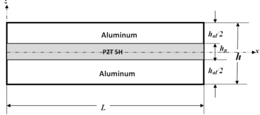
Figure 3: Geometry of a sandwich shear mode beam.

The geometric properties of the beam are:h

p =9mm, hal =9mm .

The material properties of the beam are (Kapuria and Hagedorn, 2007): Aluminum:

E

₌70.3

GPa

_;

_!

₌_0.345;

_"

₌₂₇₁₀

k

_gm

!3

PZT 5H: C₁₁=C₂₂=126GPa;C

31

=

e

32

=

#8

Fm

#1

;

!

=

7500

k

_gm

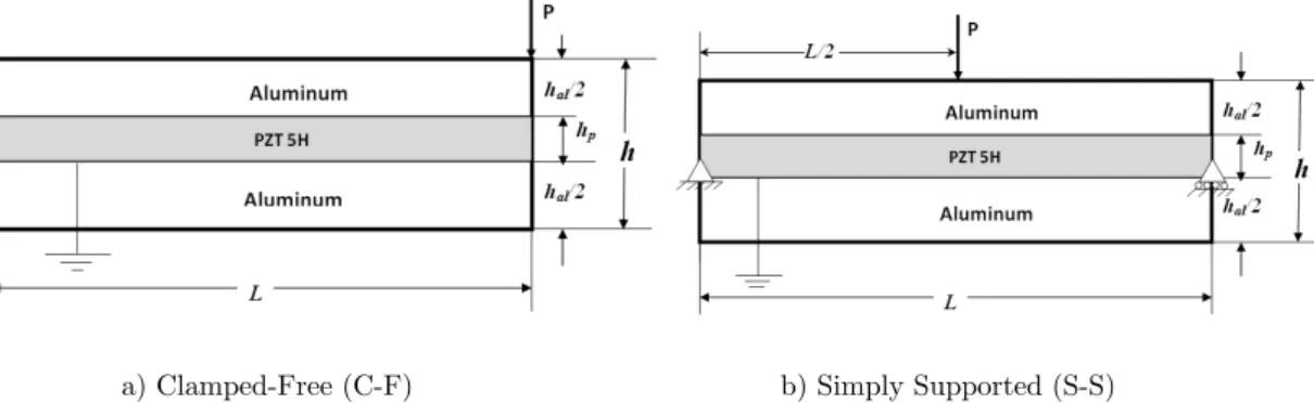
#3

Two sets of mechanical boundary conditions are considered here: (a) Clamped-Free (C-F): u_,w_,u!₌₀, at the clamped end.

(b) Simply Supported (S-S): u,w₌0, at both ends.

For simulation in ANSYS software, each aluminum layer is meshed with PLANE 183 element with 9 elements along the thickness and piezoelectric core with PLANE 223 element with 18 ele-ments along the thickness. One element per mm along the length of the beam is used for all simu-lations.

7.1 Static Analysis: Sensor Configuration

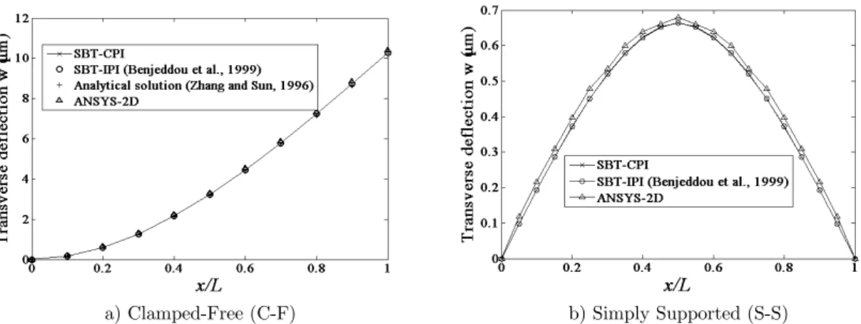
In this section, the beam shown in Figure 3 is evaluated for mechanical loading with clamped free (C-F) and simply supported (S-S) boundary conditions. The bottom surface of piezoelectric layer is grounded and a load of P=1000 N is applied at the free end for cantilever beam while at midspan for simply supported beam as shown in Figure 4. The results for maximum transverse deflection and potential developed in the beam with different aspect ratios are plotted in Figures 5 and 6, respectively for both beams. The thicknesses and composition of materials in the cross section is kept constant while length (L) is varied to obtain results for different L/h ratios. As seen from the plots, results by present SBT-CPI match with the results from analytical solutions by Zhang and Sun (1996), SBT-IPI of Benjeddou et al. (1999) and ANSYS 2D simulations.

(14)

field are plotted in Figures 9, 10 and 11, respectively. These results prove the validity of present SBT-CPI in sensor configuration.

a) Clamped-Free (C-F) b) Simply Supported (S-S)

Figure 4: Sandwich shear mode beam in sensor configuration.

Figure 5: Sensor configuration: Variation of maximum transverse deflection for various aspect ratios.

(15)

Figure 7: Sensor configuration: Variation of transverse deflection along the length of sandwich beam.

Figure 8: Sensor configuration: Variation of potential developed across piezoelectric layer along the length of sand-wich beam.

(16)

Latin American Journal of Solids and Structures 11 (2014) 1864-1885 a) Clamped-Free (C-F) b) Simply Supported (S-S)

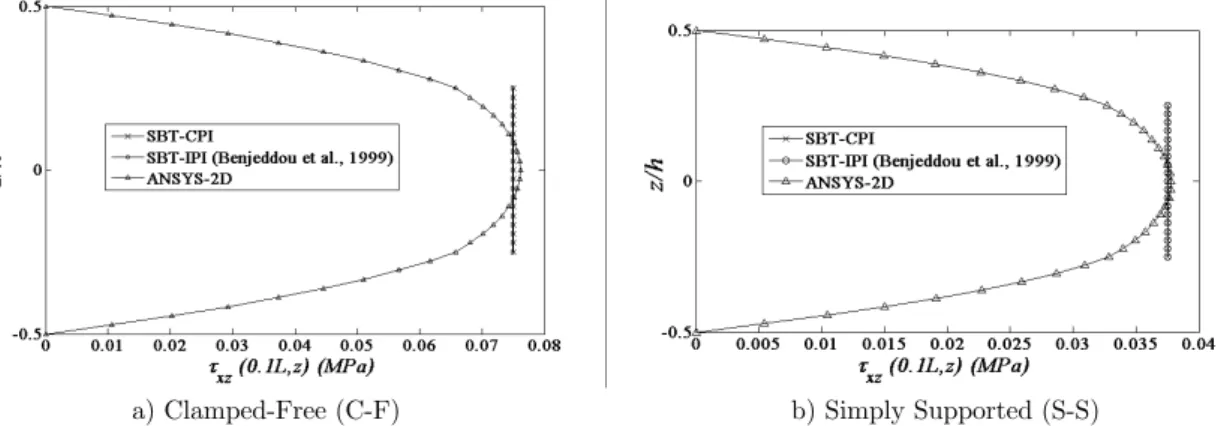
Figure 10: Sensor configuration: Through-thickness variation of shear stresses in the sandwich beam.

a) Clamped-Free (C-F) b) Simply Supported (S-S) Figure 11: Sensor configuration: Through-thickness variation of electric field in the sandwich beam.

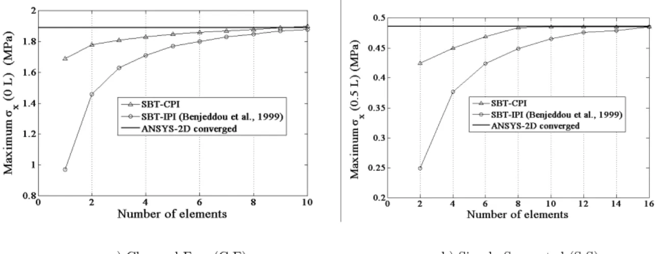
Now the efficiency of the present SBT-CPI over the conventional formulation is proved by the con-vergence graphs plotted in Figures 12 and 13 for transverse deflections and stresses, respectively. These graphs prove the superiority of the present coupled polynomial based interpolation over the conventional independent polynomial based interpolation.

(17)

Figure 13: Sensor configuration: Convergence characteristics of SBT based finite element models to predict the stress developed in the shear mode sandwich beam.

7.2 Static Analysis: Actuator Configuration

The beam shown in Figure 3 is actuated by applying voltages of ±10voltsat the top and bottom faces of the piezoelectric core for the clamped-free and simply supported boundary conditions, as shown in Figure 14. The distributions of transverse deflection along the length of the sandwich beams with

L

₌

100 mm

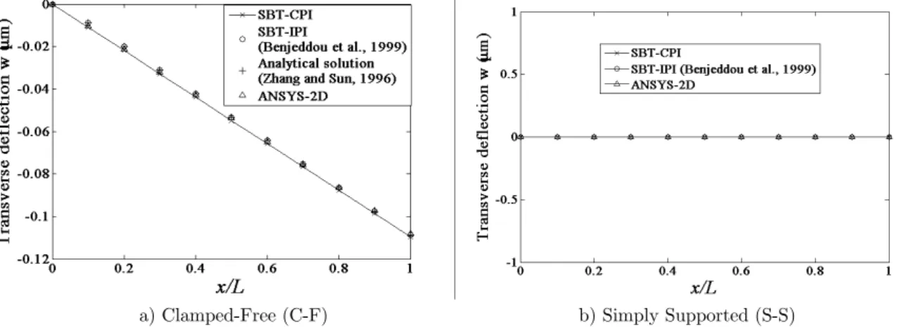
are shown in Figure 15. As seen from the graphs, for simply supported boundary condition, shear mode beams cannot produce transverse deflection which coincides with the findings by Beheshti-Aval et al. (2013). The values of tip deflection for various aspect ratios for cantilever beam are plotted in Figure 16. Also, the through-thickness variations of stresses and electric displacement developed in cantilever beam with

L

₌

100 mm

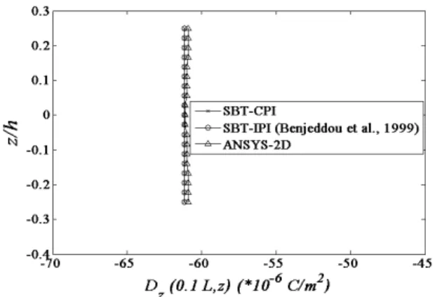
are plotted in Figures 17 and

18, respectively. Results shown in these plots validate the use of present SBT-CPI in actuator configuration.

Figure 14: Sandwich shear mode beam in actuator configuration.

(18)

pre-Latin American Journal of Solids and Structures 11 (2014) 1864-1885

sent SBT-CPI shows quick convergence while conventional SBT-IPI takes a number of elements. This proves the efficiency of the present coupled polynomial field interpolation scheme over con-ventional assumed independent polynomial based interpolations.

Figure 15: Actuator configuration: Variation of transverse deflection along the length of sandwich beam.

Figure 16: Actuator configuration: Variation of tip deflection of clamped-free (C-F) sandwich beam for various aspect ratios.

a) Axial stress b) Shear stress

(19)

Figure 18: Actuator configuration: Through-thickness variation of electric displacement developed in the C-F sandwich beam.

a) Tip deflection b) Axial stress

Figure 19: Actuator configuration: Convergence characteristics of SBT based finite element models to predict finite element results for the shear mode sandwich beam.

7.3 Modal Analysis

The developed formulation is tested here for accuracy and efficiency to predict the natural frequen-cies of the shear mode sandwich beam shown in Figure 3. The first three natural frequenfrequen-cies are evaluated in open circuit electrical boundary condition, in which bottom face of the piezoelectric layer is grounded while the top surface is left free. The converged results obtained by present SBT-CPI, tabulated in Table 1 show good agreement with the results by SBI-IPI of Benjeddou et al. (1999) and ANSYS 2D simulation. This validates the use of present coupled shape function to gen-erate consistent mass matrix also.

C-F S-S

Reference First Second Third First Second Third

SBT-CPI 1044 6107 8572 2892 10813 25784

ANSYS 2D simulation 1043 5960 8536 2803 9720 26642

SBT-IPI (Benjeddou et al., 1999) 1055 6168 8960 2921 10881 26884

(20)

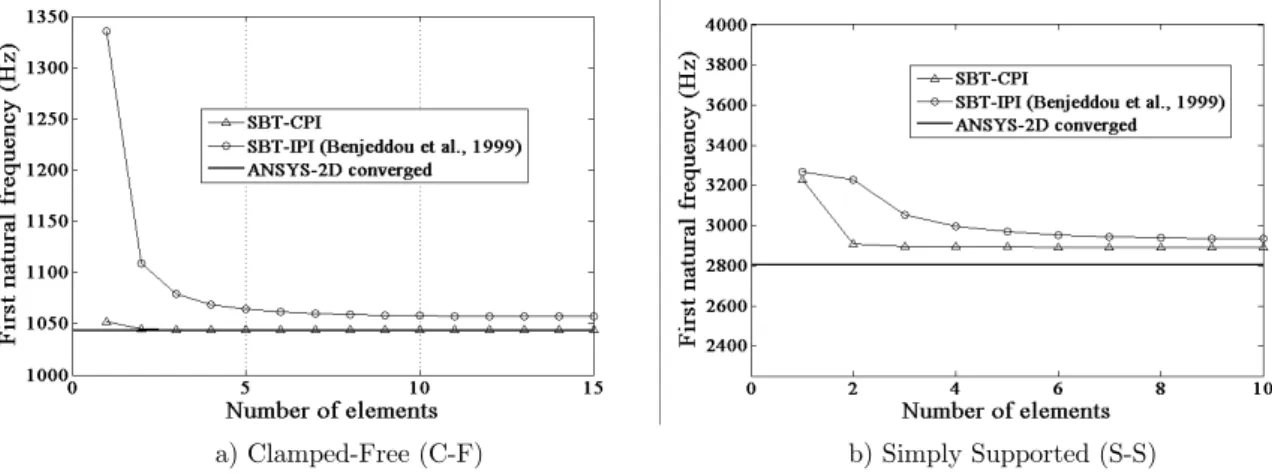
a) Clamped-Free (C-F) b) Simply Supported (S-S) Figure 20: Convergence characteristics of SBT based finite element models to predict

the first natural frequency of the shear mode sandwich beam (h_p=9mm,h_al =9mm,L=100mm).

The advantage of present coupled field interpolation over conventional independent field interpola-tion is depicted by convergence graph for first natural frequency plotted in Figure 20. The SBT-CPI converges quickly unlike SBT-IPI which takes a number of elements to reach the accurate value of first natural frequency. The first three bending mode shapes for the cantilever sandwich beam, are shown in Figure 21.

Figure 21: Natural bending modes of the shear mode sandwich beam with clamped-free boundary condition.

8 CONCLUSION

(21)

accommoda-Latin American Journal of Solids and Structures 11 (2014) 1864-1885

te shear deformation and electromechanical coupling at the field interpolation level, in a variatio-nally consistent manner. This novel way of coupled field interpolation imparts the proposed finite element improved convergence properties in comparison with the conventional SBT-based finite elements. The formulation is devoid of any locking effects and apparently the only SBT-based shear mode piezoelectric beam element which gives a single element convergence for deflection of the cantilevered sensor (tip loaded) and actuator configuration. The numerical results for the test problems applied to static and modal analyses prove the efficacy of the present formulation in modeling shear mode piezoelectric sandwich beams.

References

Abramovich, H. (2003). Piezoelectric actuation for smart sandwich structures-closed form solutions, J. Sandwich Structures and Materials 5:377-396.

Aldraihem, O.J., Khdeir, A.A. (2000). Smart beams with extension and thickness-shear piezoelectric actuators, Smart Materials and Structures 9:1-9.

Aldarihem, O.J., Khdeir, A.A. (2003). Exact deflection solutions of beams with shear piezoelectric actuators, Interna-tional J. Solids and Structures, 40:1-12.

Aldraihem, O.J., Khdeir, A.A. (2006). Analytical solutions of antisymmetric angle ply laminated plates with thick-ness-shear piezoelectric actuators, Smart Materials and Structures 15:232-242.

Aldraihem, O.J., Khdeir, A.A. (2012). Analytical solution of Reddy’s third-order laminates with shear piezoelectric layers, Mechanics of Advanced Materials and Structures 19:18-28.

Baillargeon, B.P., Vel, S.S. (2005). Active vibration suppression of sandwich beams using piezoelectric shear actua-tors: experiments and numerical simulations, J. Intelligent Material Systems and Structures 16:517-530.

Beheshti-Aval, S.B., Shahvaghar-Asl, S., Lezgy-Nazargah, M., Noori, M. (2013). A finite element model based on coupled refined high-order global-local theory for static analysis of electromechamical embedded shear-mode piezoe-lectric sandwich composite beams with various widths, Thin-Walled Structures 72:139-163.

Benjeddou, A., Trindade, M.A., Ohayon, R. (1997). A uniﬁed beam finite element model for extension and shear piezoelectric actuation mechanisms, J. Intelligent Material Systems and Structures 8:1012-1025.

Benjeddou, A., Trindade, M.A., Ohayon, R. (1999). New shear actuated smart structure beam finite element, AIAA J. 37:378-383.

Benjeddou, A., Trindade, M.A., Ohayon, R. (2000). Piezoelectric actuation mechanisms for intelligent sandwich structures, Smart Materials and Structures 9:328-335.

Crawley, E.F., de Luis, J. (1987). Use of piezoelectric actuators as elements of intelligent structures, AIAA J. 25: 1373-1385.

Edery-Azulay, L., Abramovich, H. (2004). Piezoelectric actuation and sensing mechanisms-closed form solutions, Composite Structures 64:443-453.

Kapuria, S., Hagedorn, P. (2007). Unified efficient layerwise theory for smart beams with segmented exten-sion/shear mode, piezoelectric actuators and sensors, J. Mechanics of Materials and Structures 2:1267-1298. Khdeir, A.A., Aldraihem, O.J. (2001). Deflection analysis of beams with extension and shear piezoelectric patches using discontinuity functions, Smart Materials and Structures 10:212-220.

(22)

Latin American Journal of Solids and Structures 11 (2014) 1864-1885 Raja, S., Pratap, G., Sinha, P.K. (2002). Active vibration control of composite sandwich beams with piezoelectric extension-bending and shear actuators, Smart Materials and Structures 11:63-71.

Rathi, V., Khan, A.H., (2012). Vibration attenuation and shape control of surface mounted, embedded smart beam, Latin American J. Solids and Structures 9: 401-424.

Raveendranath, P., Singh, G., Pradhan, B. (1999). A two-noded locking-free shear flexible curved beam element, International J. Numerical Methods in Engineering 44:265-280.

Raveendranath, P., Singh, G., Pradhan, B. (2000). Application of coupled polynomial displacement fields to lami-nated beam elements, Computers and Structures 78:661-670.

Sulbhewar, L.N., Raveendranath, P. (2014a). A novel efficient coupled polynomial field interpolation scheme for higher order piezoelectric extension mode beam finite elements, Smart Materials and Structures 23:25024-25033. Sulbhewar, L.N., Raveendranath, P. (2014b). An accurate novel coupled field Timoshenko piezoelectric beam finite element with induced potential effects, Latin American J. Solids and Structures 11:1628-1650.

Sun, C.T., Zhang, X.D. (1995). Use of thickness-shear mode in adaptive sandwich structures, Smart Materials and Structures 4:202-206.

Trindade, M.A., Benjeddou, A. (2006). On higher-order modelling of smart beams with embedded shear-mode piezoceramic actuators and sensors, Mechanics of Advanced Materials and Structures 13:357-369.

Trindade, M.A., Benjeddou, A. (2008). Refined sandwich model for the vibration of beams with embedded shear piezoelectric actuators and sensors, Computers and Structures 86:859-869.

Vel, S.S., Batra, R.C. (2001). Exact solution for the cylindrical bending of laminated plates with embedded piezo-electric shear actuators, Smart Materials and Structures 10:240:251.

Zhang, X.D., Sun, C.T. (1996). Formulation of an adaptive sandwich beam, Smart Materials and Structures 5: 814-823.