J. of the Braz. Soc. of Mech. Sci. & Eng. Copyright 2003 by ABCM July-September 2003, Vol. XXV, No. 3 /
R. T. Coelho,
A. Braghini Jr.,
C. M. O. Valente and
G. C. Medalha
Department of Production Engineering School of Engineering at São Carlos University of São Paulo, São Carlos SP, 13.566-590. Brazil [email protected]
Experimental Evaluation of Cutting
Force Parameters Applying
Mechanistic Model in Orthogonal
Milling
There have been considerable efforts in research to understand the basics of chip formation. Models developed for turning and adapted to milling, yield reasonable results, except in some particular applications. This work develops an experimental method capable of providing cutting data in a fast and reliable way to evaluate the specific cutting presure(Ks), the friction coefficient (µ) and the ploughing/elastic forces
(FE). Different models for the cutting force can be tested, and the coefficient of
determination (R2) assesses the adequacy of models. The particular adopted model, used to test the experimetal method hereby proposed, resulted in a good agreement with experimental data, expressed by R2 values very close to the unity
Keywords: Machining, milling, simulation, orthogonal cutting
Introduction
Machining is undoubtedly the most important of the basic manufacturing processes, since industries around the world spend billions of dollars per year to perform metal removal (DeGarmo et al. 1997). That is so, because the vast majority of manufactured products require machining at some stage in their production, ranging from relatively rough operations to high-precise ones, involving tolerances of 0.001 mm, or less, associated with high-quality surface finish. It is estimated that today, in industrialized countries, the cost of machining accounts to more than 15% of the total value of all products by their entire manufacturing industry, whether or not these products are mechanical (Merchant 1998).
1
There have been considerable efforts in research and experimentation throughout the 20th century aiming at understanding the basics of the process, particularly the chip formation. Models have been proposed to explain the phenomena occurring when material is removed from the workpiece in the form of chips. Researches into chip formation in metals had been carried out as far back as 1873, but fundamental theories and models seem to have appeared at the beginning of the 20th century only (Kronenberg 1966). The first important concepts were the existence of a shearing plane and the chip compression factor, which would be always greater than the unity. The simplifications introduced with the study of orthogonal cutting were also important because they contributed to an easy understanding and to the introduction of a 2D model for velocities and forces. The fundamental parameter of this model was the shear angle, which soon proved to be of difficult prediction. Many researchers proposed several relations, which are detailed in a number of reviews (Kronenberg 1966, Ehmann et al. 1997). Later, however, the shear plane was admitted to have a “thickness” (Oxley et al. 1963) and was called the shear zone where there was a hydrostatic pressure acting. In other early models the radius of the cutting edge, initially equaled to zero, became important (Albrecht 1960), as well as, the friction at the interface tool-chip and tool-machined surface. These models added more accuracy to the prediction of shear angle and, consequently, to the prediction of forces in
Paper accepted June, 2003. Technical Editor: Alisson Rocha Machado.
machining. Recently, mathematically more detailed and specific models have been proposed including effects of the cutting edge radius (Waldorf, et al 1998, Waldorf et al. 1999) and material behavior with temperature effects (Oxley 1998, Özel and Altan 2000). Models have also been proposed to explain chip formation even in precision machining (Arcona et al. 1998) where depths of
cut are around 0.5 µm. Some models aimed at the prediction of
machining performance, besides forces and speeds (Amarego 1998, Kapoor et al. 1998). Broader models for chip formation have been proposed for encompassing the small chips formed in abrasive processes, such as grinding (Shaw 1996). In these processes the chips are formed more like an extrusion process near the radius of the cutting edge, because the rake angle is highly negative.
Milling, for example, has its own particularities, such as variation on the undeformed chip thickness (h), interrupted cuts, etc. Models developed for turning and adapted to milling, working with average chip thickness, can yield reasonable results in terms of force. There are operations, however, where a more accurate result is needed and then, the discrepancies may become unacceptable. That is the case with high speed milling, which uses very low chip thickness. In this case, the cutting edge radius almost equals the undeformed chip thickness and the rake angle tends to be highly negative. The material seems to be removed like in abrasive processes (Shaw 1996). Additionally, the main parameters describing the models are a function of other ones related to the tool (material, geometry, coating, etc.) and the machine (rigidity, speed, position control, etc.). In order to investigate the end milling process in some cutting conditions, at any particular combination tool-machine-workpiece, a simple and fast method is needed to find the main parameters of the classical existing models and study some new ones.
Nomenclature
A = Cross sectional area of the chip
C = Constant at the Equation (3)
Cp = Cutting force coefficient to a specific cutting pressure at Equation (2)
FC= force acting at the cutting speed direction
FEC = Elastic force component acting at the cutting direction
FER = Elastic force component acting perpendicular to the cutting direction
FH = force acting at the horizontal direction
FR= force acting perpendicular to the cutting speed direction
FV = force acting perpendicular to the horizontal direction
KAB = Shear flow stress at Equation (3)
KS = Specific cutting pressure
R2 = Coefficient of determination
Rc = Cutter radius
f = feed rate
h = undeformed chip thickness
n = Strain-hardening index
npt = Number of points acquired
stp = step used to increment the angular position of the cutting edge
t1 = undeformed chip thickness in Equation (3)
w = Cutting width
zp = Exponent at Equation (2)
µ = Apparent coefficient of friction
θ = Angular position of the cutting edge\
φ = Shear plane angle
ε = Strain
σ = Stress (flow or principal)
Force Models
There are several models suggested by a number of authors throughout the 20th century, which could be tested against the acquired data. They have many common aspects and most of them include some very specific particularities. First models, at the beginning of the century, proposed a direct relation between forces and the chip cross sectional area (Kronenberg 1966, Ehmann et al. 1997, Waldorf et al. 1998), in general equations like:
A K
Fc = s⋅ (1)
where Ks is the specific cutting pressure and A is the cross
sectional area of the undeformed chip. This equation came from observations that there seems to be an approximate linear relation between force and area in some experimental data, mainly from turning. Later on, it was found that Ks is not constant, but rather a function of process parameters, such as chip thickness and rake angle, for example. Kronenberg (1966), proposed a more detailed equation for Ks, which was:
zp p
s C A
K = (2)
where Cp was a Cutting Force Coefficient to a unity of cutting force and the exponent (zp) is an experimental value depending on tool-workpiece pair. Following on, many other researchers proposed
equations for Ks even including some other parameters, such as
feed and depth of cut. Every new parameter seems to have added
more complexity to the equation and little more accuracy on the prediction of experimental data. Later on, Oxley et al. (1963) proposed a more detailed model based on the equation:
) n , C , ( wf t K
Fc = AB1 φ (3)
where KAB is the shear flow stress along the shear zone, t1 is the
undeformed chip thickness, w is the cutting width, f(φ,C,n) is a
function of the shear plane angle, C is the constant in the empirical strain-stress relation and n is the strain-hardening index of the
empirical stress/strain relation ( n
1ε
σ
σ = ).
Some other equations, such as the one proposed by Albrecht (1960), included the ploughing component to the cutting force, which is more significant when the values of depth of cut approach the edge radius. A more comprehensive study of the effects of this component in the cutting force was published later (Waldorf et al. 1998, Waldorf et al. 1999), starting from the forces components on the shear plane and rotating them to the direction of the cutting speed and perpendicular to it. Equation for the ploughing component were based on three physical models: Slip-Line, a Separation Point on the Edge and a stable Built-up on the Edge. These models give three different equations with several parameters, which depend on the material properties and on the yield stress. Some other slightly different models have been proposed for explaining chip formation in precision machining, such as that described in Arcona et al. (1998). In all models, analyzed at the present work, the tangential force component (or thrust force), perpendicular to the cutting speed direction, was a function of the cutting force.
The present work is aimed at the development of an experimental method that is capable of providing cutting data in a very fast and reliable way using several different cutting conditions for each particular combination of tool-machine-workpiece. It can be used to evaluate the specific cutting pressure (Ks), the friction coefficient (µ) and the ploughing, or elastic forces (FE), for
example, but also to test new equations and models. All the
equations are solved using numerical methods, to give the most precise solution using simple software. A particular simple model is used to test the practicality of the experimental method.
Description of the Method
The method consists of performing an orthogonal milling operation using an end mill fitted with a single point indexable insert. Force is measured and recorded during the cut. With the acquired data, an average curve of force is made using 5 consecutive rotations. An adopted simple model of force, as a function of the undeformed chip tickness (h), is fitted into the force data. To fit the curves, the best values of main parameters are calculated.
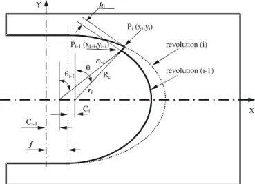
J. of the Braz. Soc. of Mech. Sci. & Eng. Copyright 2003 by ABCM July-September 2003, Vol. XXV, No. 3 / revolution (i) revolution (i-1) Rc Ci-1 Ci f θi-1 θi
Pi (xi,yi)
hi
Y
X Pi-1 (xi-1,yi-1)
ri
ri-1
Figure 1. Schematic of the movements of the cutting edge on the workpiece for two consecutive turns of the end mill.
According to Fig. 1, taking the angle θi-1 and the correspondent position of the center of the end mill, Ci-1, the points of the curve, P(xi-1,yi-1), at the turn (i-1) are:
1
1 cos −
− = c i
i R
y θ (4)
(
)
11
1 − 2 −
− = c i + i
i R sin f
x θ πθ (5)
where Rc is the radius of the end mill. Ci-1 is the displacement of the center, which can be calculated by:
(
)
11 2 −
− = i
i f
C π θ . (6)
When the cutting edge is at the next revolution, the angle is θi and the correspondent center position is Ci. At this revolution, with the angle being θi, the points of the curve P(xi,yi) described by the cutting edge, at the revolution i are:
i c
i R
y = cosθ (7)
(
f)
fsin R
xi = c θi + 2π θi + (8) At the angle θi-1 there is a line ri-1 described by the following equation:
ri-1 =>
− − = − − − − − 1 1 1 1 1 2 2 i i i i i tg f x tg y θ π θ θ π (9)
At the angle θi there is also a line ri described by the following equation:
ri =>
i i i i i tg f x tg y θ π θ θ
π − + − = 2 1 2 (10)
Taking the generic position illustrated in the Fig. 1, it can be noted that the point Pi-1 belongs to both lines. Using this condition, the point Pi-1 is placed at the Eq. (10) and then substituting Eq. (4) and Eq. (5), results in:
0 2 1 2 ) ( 2
cos 1 1 1 =
+ + + − − − − − i i i i c i i c tg f f sin R tg R θ π θ θ π θ θ π θ (11)
Equation (11) cannot be directly solved and numerical methods should be used. The numerical method used was the Bracketing and Bisection, well described in Press et al. (1989) and Cunha (1993). When Eq. (11) is solved, the angle θi-1 is found for a given
θi. At this stage the points Pi and Pi-1 can be found using Eq. (4), (5), (7) and (8). The undeformed chip thickness is the distance hi given by:
(
) (
)
21 2
1 −
− − −
−
= i i i i
i x x y y
h (12)
Using angles varying according to a step determined by the number of points acquired in one revolution (Eq. (20)), the pairs of values (hi ,θi) can be found.
Despite of all the existing models, for the present work, a simple one was used to test the experimental proposed method. Some others could be used, slightly changing the equations to solve the Least Square Method. Accordingly, the force acting on the workpiece is made of two components: the cutting force, FC, in the
direction of the cutting speed, and the radial force, FR, in the
perpendicular direction. The component FC is proportional to the
undeformed chip thickness and FR depends on an apparent
coefficient of friction (µ) between the chip and the tool rake face.
That can be used when the rake angle is going to be 0°. Both
components are calculated as follows:
EC S
Ci K wh F
F = . . + (13)
ER Ci
Ri F F
F = .µ + (14)
Both force components have an elastic-plastic part, as suggested by Arcona et al. (1998) and similar to the ploughing part, which are responsible for that portion of metal not being sheared, but “extruded” throughout the cutting edge radius. These components (FEC and FER) are the elastic-plastic deformation of the metal and depend on the tool radius, the mechanical properties of the workpiece material and so on, also described by Zimerman et al. (1970). For a given pair tool-workpiece, at some fixed cutting conditions, these components can be reasonable represented by a constant value. During the experimental tests the cutting edge is rotated and the tool center is continuously moving, therefore the direction of the machining force components are constantly changing direction (and values). The dynamometer measures force components in a vertical (FV) and horizontal (FH) direction. In order to be able to match the forces registered by the dynamometer and those calculated by the Eq. (13) and (14) these have to be rotated according to the angle of the tool (θi). Fig. 1 illustrates this situation.
Using the rotational matrix applied to the components acting on the cutting edge, the measured ones can be obtained as follows:
Vi Hi Ri Ci i i i i F F F F sin sin =
− θ θ
θ θ
cos cos
(15)
i Ri i Ci
Hi F F sin
F = cosθ + θ (16)
i Ri i Ci
Vi F sin F
F =− θ + cosθ (17)
By substituting Eq. (13) and (14) into (16) and (17) yields:
(
s i EC)
i s i EC ER iHi K wh F K wh F F sin
F = . . + cosθ +( . . .µ+ .µ+ ) θ (18)
(
s i EC)
i s i EC ER iVi K wh F sin K wh F F
F = − . . + θ +( . . .µ+ .µ+ )cosθ (19)
With these equations, the experimentally obtained points are fitted to them and the values of the parameters Ks, FEC and µ are found for each pair tool-workpiece. These equations can be applied to any combination of tool material, workpiece and cutting conditions. It also has to be emphasised that FVi and FHi are related each other and just one of them could be enough.
The method used at the present work to fit the equations is the Least Square Method (LSM) (Press et al. 1989, Cunha 1993). When the LSM coefficients are found the functions are fitted on the
experimental points and a coefficient of determination R2 (Hines
and Montgomery 1990) is then, calculated to assess the adequacy of the regression model. This coefficient is the square of the correlation coefficient between model points and measured ones. The better the regression model is, the closest R2 is to the unity.
To synchronize the force signals and the angular position of the cutting edge a magnetic sensor (model Sense PS2-12GM50A2-V1) was used, shown in Fig. 2. This was needed to establish the force value at the exact position of zero radians of the cutting edge.
Each experiment started fixing one of the cutting conditions, force data and synchronization signal acquisition with the end mill fully into the test piece. The data were recorded into a file in text format (ASCII), which was also used to see the graph of force components and synchronization signal against tool rotation angle (θi). The step (stp) for this angle was calculated by the following equation:
PT
n
stp= 2π (20)
where nPT is the number of points acquired in one revolution, taken between two consecutive rise in the synchronization signal.
Experimental Set Up
Figure 2 shows the set up used in a CNC machining center.
Figure 2. Schematic of the set up used in a CNC machining center.
All experiments were performed in a machining center model VARGA MFH40, 10 kW, 5,000 rpm maximum spindle rotation, equipped with CNC Siemens Sinumerik 3M. The end mill was a 25 mm diameter code R216.2-025. Force data came from a 3D (X,Y,Z) Kistler dynamometer type 9257BA with control unit for dynamometer with built-in charge amplifier type 5233A. Data acquisition card was a PCI-MIO-16E4 with maximum acquisition rate of 250,000 samples per second. The digital data was acquired with 10,000 samples per second, which proved to be high enough to give reliable information during one revolution of the end mill. The data was processed in Microsoft® Excel 97. The acquisition software was developed using LabView 5.1 program. Each run of the experiment takes about 60 seconds. The test piece design was developed for the special purpose of this experiment and is shown in Fig. 2. It was used test pieces of AISI 1045 with thickness of 1.5 and 3.0 mm at the useful area.
Results and Discussion
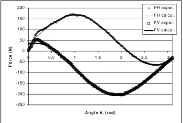
Analysis of the Adequacy of the Model
Figs. 3 and 4 show the curves obtained from the experimental (exper.) and calculated (calcul.) points for the horizontal (FH) and vertical (FV) force components.
-250 -200 -150 -100 -50 0 50 100 150 200
0 0,5 1 1,5 2 2,5 3
A n g l e θθi ( r a d )
Force (N)
FH exper.
FH calcul.
FV exper.
FV calcul.
Figure 3. Curve from experimental and calculated data for v = 75 m/min, f =
J. of the Braz. Soc. of Mech. Sci. & Eng. Copyright 2003 by ABCM July-September 2003, Vol. XXV, No. 3 /
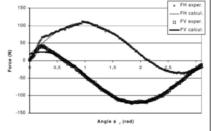
In general, for all experiments, it was observed that the regression model shows excellent fitting, with regression coefficient values of 0.995, 0.933, respectively, for horizontal and vertical force component of data shown in Figure 3 and 0.990 and 0.989 for the same data in Fig. 4. At the beginning of the curves, for small angles at the entrance of the tool, there is a slight difference between experimental and calculated curves. At the entrance, the cutting edge starts to rub the workpiece surface and the undeformed chip thickness is nearly zero. Following on, as the thickness grows there is a sharp increase in the force, especially in the vertical component. Until the force is capable of reaching a value high enough to cause rupture on the workpiece material, there will be no chip formed. At a certain point, the material starts to flow (the flow stress has been reached at the small contact area) and forces become relatively stable. After that, there is rupture and chips actually are formed following the classical shearing model. This effect is stronger for low feed rate values, where the tool has to cover more angular rotation to reach the critical turning point for chip formation. One experiment was performed using feed rate as low as 0.010 mm/rev. The resulting curves are shown in Fig. 5.
-150 -100 -50 0 50 100 150
0 0,5 1 1,5 2 2,5 3
A n g l e θθ i (rad)
Force (N)
FH exper.
FH calcul.
FV exper.
FV calcul.
Figure 4. Curve from experimental and calculated data for v = 75 m/min, f =
0.025 mm/rev and w = 1.5 mm. Material AISI 1045 (bold).
-80 -60 -40 -20 0 20 40 60 80 100
0 0,5 1 1,5 2 2,5 3
angle (θθi)
Force (N)
FH exper. FH calcul. FV exper. FV calcul.
Figure 5. Curve from experimental and calculated data for v = 50 m/min, f =
0.010 mm/rev and w = 1.5 mm. Material AISI 1045.
Another aspect observed in very low feed rate values was that the tool has its own rigidity, which allows deformation at the same magnitude of the undeformed chip thickness, when subjected to forces found during the cut. This could lead to revolutions of the tool without actually removing any material. At the subsequent revolution, however, there will be an accumulated spring effect, which will act as a disturbance on the real undeformed chip
thickness. This was observed by the fact that there is variation on the maximum value of the force components from one turn to the next, when feed rate set was less than 0.025 mm/rev.
Because the regression model starts at an angle of zero radians and at this point the theoretical undeformed chip thickness is not zero, there is already force acting. Its value is mainly due to the friction and at this point there is no chip being formed by shearing, but perhaps, the material is subjected to a drawing process. This could be precisely determined because of the synchronization signal coming from the magnetic sensor, see Fig. 1. This sensor was calibrated and its repeatability resulted in 10 µm, which means 0.006 degrees in angular position for the end mill.
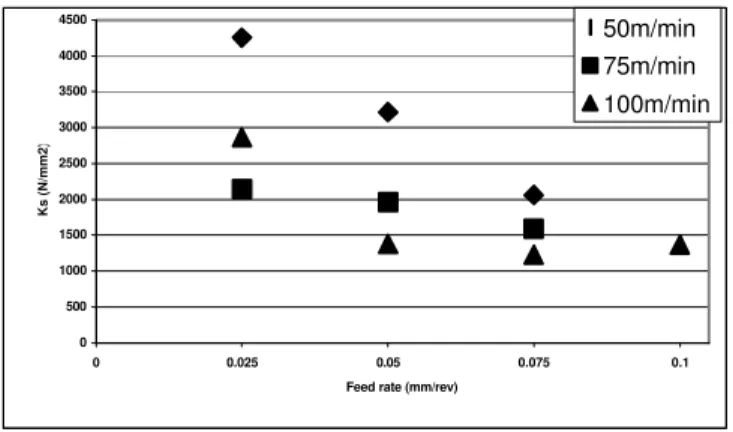
Analysis of the Specific Cutting Pressure (Ks)
In general, the specific cutting pressure shows significant variations, according to the cutting speed, feed rate and also cutting width. Its value increases for small values of feed rate, for high values of cutting speed and cutting width. Low values of feed rate indicate that the shear model could not fit adequately the chip formation process, since the material is subjected to lower strain rates. In this way the values of the specific cutting pressure tends to increase. As an example, the values obtained when using feed rate
as low as 0.010 mm/rev were 5139 and 5501 N/mm2, for cutting
width of 1.5 and 3.0 mm, respectively. The variation of Ks with the cutting speed is not strong, but it seems to be related to the cutting temperature, since both have a direct relationship. The cutting speed range used was not large enough to cause significant
temperature variation, but values of Ks for higher speeds lie
predominantly low in the graphs of Figures 6 and 7. For higher values of cutting speed, Ks seems to be independent of the cutting width, but for 50 m/min the values obtained using cutting width of 3.0 mm, were much higher than those with 1.5 mm. This could be attributed to the higher energy need for deformation on the tool, since the elastic components were, in general higher in those experiments using cutting width 3.0 mm.
0 500 1000 1500 2000 2500 3000 3500 4000 4500
0 0.025 0.05 0.075 0.1
Feed rate (mm/rev)
Ks (N/mm2)
50m/min
75m/min
100m/min
0 500 1000 1500 2000 2500 3000 3500 4000 4500
0 0.025 0.05 0.075 0.1
Feed rate (mm/rev)
Ks (N/mm2)
50m/min 75m/min 100m/min
Figure 7. Specific cutting pressure as a function of the feed rate and cutting speed using cutting width 3.0 mm.
Both graphs seem to indicate that the values of Ks will
converge to around 1500 N/mm2, as feed rates become higher than
0.1 mm/rev. These cutting conditions could not be tested, due to chatter, and excessive forces on the dynamometer. These instabilities could also be accounted for the dispersion observed when the cutting width was 3.0 mm. The set tool-workpiece-dynamometer was not rigid enough to withstand the forces imposed by the havier cutting conditions.
Analysis of the Coefficient µµ
An average value of µ was calculated using the results obtained with both force components. The graphs are shown in Figs. 8 and 9.
The coefficient µ was introduced into the model as parameter
similar to the friction coefficient, although it is not a direct relation between both components of the cutting force. It resulted to be almost constant with feed rate and cutting speed, within a certain range for each cutting width, except for the higher value of cutting speed. At 100 m/min the values of µ are much higher, meaning that it might be strongly influenced by speed. Since it multiplies the cutting force component, Eq. (2), at such conditions, it makes the radial component higher, indicating that it must be higher in order to produce chip.
0 0.5 1 1.5 2 2.5 3 3.5
0 0.025 0.05 0.075 0.1
Feed rate (mm/rev)
Values of
µµ
50m/min 75m/min 100m/min
Figure 8. Values of the coefficient as a function of feed rate and cutting speed for cutting width of 1.5 mm.
0 0.5 1 1.5 2 2.5 3 3.5
0 0.025 0.05 0.075 0.1
Feed rate (mm/rev)
Values of
µµ
50m/min 75m/min 100m/min
Figure 9. Values of the coefficient µµ as a function of feed rate and cutting
speed for cutting width of 3.0 mm.
Final Considerations
These results also confirms the need for an experimental method to evaluate the unity cutting force for each particular situation, since the models so far presented have not been able to precisely predict cutting forces. Additionally, the experimental results clearly show that the specific cutting pressure is not a material constant, but a function of several input parameters, such as cutting speed, feed rate, tool material, tool geometry, machine rigidity, etc. Even FEM models cannot precisely predict cutting forces based only on general equations and material constants, as the differences observed in Özel and Altan (2000) and also in Fuh and Hwang (1997).
The other parameters obtained with the fitted model (FER and
FEC) seem also to have significant variations according to the input parameters. They will have to be studied on other models and tested in the future. The new models to be tested will need more accurate studies of these elastic-plastic forces and their role on the chip formation process and, consequently, on the cutting force, according to feed rate and cutting speed. The model proposed in the present work seems to be good enough to explain cutting force for feed rates as low as 0.025 mm/rev. Below this values, were edge radius starts to play a more significant role on the chip formation process, new ideas will have to be tested. New models will be proposed for these situations, mainly if these are to be applied to high-speed cutting processes. The association of high cutting speed and very low feed rate and depth of cut will have to be studied in more details in order to find a better chip formation model. The way appears to be on the plasticity theory with methods applied to forming processes, particularly on cold drawing and extrusion. Models adopted in these forming operations may be applicable on machining, when extrusion operation is performed with very large cone angle (shaving) (Zimerman et al. 1970, Chang et al. 1960, Altan et al. 1983).
Conclusion
Since a general model of the cutting force, capable of precisely predict it for all milling operations is not available, the proposed experimental method can evaluate cutting parameters for combinations of different materials, tools, coatings, machines, etc. The method is also able to give force variations during all the cutting edge revolution, in a fast and simple way. The calculation
can be easily implemented using, for example, Microsoft Excel
J. of the Braz. Soc. of Mech. Sci. & Eng. Copyright 2003 by ABCM July-September 2003, Vol. XXV, No. 3 /
different software can be used for the regression, with some of them calculating the constants directly, using other methods besides the Least Square Method.
Different models for the cutting force can be tested, though the regression equations will be different, and the coefficient of
determination (R2) will assess the adequacy of most models. A
more complex model, using the undeformed chip thickness with an exponent, such as the model proposed by Kronenberg and Kienzle (Kronenberg 1966), was tried during the development of the present work. The solution of the equations on the Least Square Method resulted much more difficult and the values for the exponent always resulted close to 1. The coefficient of determination also improved when exponent 1 was used. Therefore, the model adopted did not include an exponent for the undeformed chip thickness (h).
The specific cutting pressure found by the regression equations shows some variation depending on the feed rate, cutting speed and cutting width. Its value increases for small values of feed rate, for high values of cutting speed and cutting width. For low values of feed rate, the chip formation process cannot be entirely explained by models based on shearing. In these conditions, force graphs indicate that the material is being deformed up to a relatively stable value, like a “flowing point” similar to the behavior observed on forming processes. At this point, the shearing models shows a poor agreement and friction and elastic-plastic behavior of the material may be more adequate, but the model needs to be found.
The simple model applied here, only to test the proposed experimental method, resulted quite well in matching the experimental data, although clearly shows that there are huge differences between the specific cutting pressure and friction coefficient, depending on cutting speed, feed rate and cutting width.
References
Albrecht, P., 1960, “New Developments in the Theory of the Metal-Cutting Process – Part I The Ploughing Process in Metal Metal-Cutting,” Journal of Engineering for Industry, Nov., pp. 348-358.
Amarego, E.J.A., 1998, “A Generic Mechanics of Cutting Approach to Predictive Technological Performance Modeling of the Wide Spectrum of
Machining Operations,” Machining Science and Technology, Vol. 2, N. 2, pp. 191-211.
Arcona, C. and Dow, Th.A., 1998, “An Empirical Tool Force Model for Precision Machining,” Journal of Manufacturing Science and Engineering, Vol. 120, pp. 700-707.
Cunha, C., 1993, Métodos Numéricos – Para engenharias e Ciências Aplicadas, Editora da Unicamp, Brazil (In Portuguese).
DeGarmo, E.P., Black, JT., and Kohser, R.A., 1997, , Materials and Processes in Manufacturing, 8th Edtion, Printice-Hall, USA.
Ehmann, K.F., Kapoor, S.G., DeVor, R.E. and Lazoglu, I., 1997, “Machining Process Modeling: A Review,” Journal of Manufacturing Science and Engineering, Vol. 119, Nov., pp. 655-663.
Fuh, K.H. and Hwang, R.M., 1997, "A Predicted Milling Force Model for High Speed End Milling Operation", International Journal of Machine Tools and Manufacture, 37, pp969-979.
Hines, W.W. and Montgomery, D.C.,1990, Probability and Statistics in Engineering and Management Science, 3rd Edtion, John Wiley & Sons, Canada.
Kapoor, S,G., DeVor, R.E., Zhu, R., Gajjela, R., Parakkal, G. and Smithey, D., 1998, “Development of Mechanistic Models for the Prediction of Machining Performance: Model Building Methodology,” Machining Science and Technology, Vol. 2, N. 2, pp. 213-238.
Kronenberg, M., 1966, Machining Science and Application – Theory and Practice fo Operation and Development of Machining Processes, 1st Edtion,
Pergamon Press, UK.
Merchant, M.E., 1998, “An Interpretative Look at 20th Century Research on Modeling of Machining,” Machining Science and Technology, Vol. 2, N. 2, pp. 157-163
Oxley, P.L.B. and Hatton, A.P., 1963, “Shear Angle Solution Based on Experimental Shear Zone and Tool-Chip Interface Stress Distribution,” International Journal of Mechanical Science, Vol. 5, pp. 41-55.
Oxley, P.L.B., 1998, “Development and Application of a Predictive Machining Theory,” Machining Science and Technology, Vol. 2, N. 2, pp. 165-189.
Özel, T. and Altan, T., 2000, "Process Simulation Using Finite Element method - Prediction of Cutting Forces, Tool Stresses and Temperatures in High Speed Flat end Milling", International Journal of Machine Tools and Manufacture, 40, pp713-738.
Press, W.H., Flannery, B.P., Teukousky, S.A. and Vetterling, W.T., 1989, Numerical recipes in Pascal – The Art of Scientific Computing, Cambridge University Press, UK.
Shaw, M.C., 1996, Principles of Abrasive Processing, 1st Edtion,,
Clarendon Press – Oxford.
Waldorf, D.J., DeVor, R.E. and Kapoor, S.G., 1998, “A Slip-Line Field for Ploghing During Orthogonal Cutting,” Journal of Manufacturing Science and Engineering, N. 120, Nov., pp. 693-699.
Waldorf, D.J., DeVor, R.E. and Kapoor, S.G., 1999, “An Evaluation of Ploughing Models for Orthogonal Machining,” Journal of Manufacturing Science and Engineering, Vol. 121, Nov., pp. 550-558.