ABSTRACT: The continued growth of the general aviation leet demands the need of forever improved preventive methods of failure analysis, in order to reduce the number of incidents or accidents. It has been proved that one possible solution to avoid unsafe conditions is the installation of new avionic systems. This article presents the method named IMFLAR — an Intuitive Method For a Logical Avionics Reliability, an analysis method for avionic systems installations based on a conceptual model of human factors and an artiicial neural network application, giving an overview of these installations and analyzing the involved risk factors. This is a new preventive approach that establishes a relationship between unsafe characteristics observed during the installation of avionic systems and an operational database of incidents and accidents, in order to provide a framework to make aviation safer. Additionally, this article describes the steps to obtain the necessary parameters that ought to be used to avoid unsafe conditions for a modiication that installs an avionics system in the aircraft.
KEYWORDS: Accidents prevention, Avionics system, Artiicial neural network.
IMFLAR: An Intuitive Method for Logical
Avionics Reliability
Nilson Silva1, Luís Gonzaga Trabasso2
INTRODUCTION
Nowadays, general aviation is the category that covers the largest number of aircrats in operation (e.g., business aircrat, charter light and agricultural).
Aircrat accidents are responsible for innumerous losses, claiming lives and causing large material damages. he Brazilian General Aviation leet is increasing, and there is a continuous technological advance that implies in crescent risk factors for incidents or accidents. For this reason, it is necessary the use of new prevention methods. hese methods must analyze relationships among the triad man-machine-environment: where man represents human factors; machine symbolizes aircrat, systems and ground/air facilities; and environmentis related to climatic and environmental factors. he triad man-machine-environment summarizes some fundamental elements in investigation of aircrat accidents and is the theme of the Centre for Research and Prevention of Aeronautical Accidents of Brazilian Air Force (CENIPA – Centro de Investigação e Prevenção de Acidentes Aeronáuticos).
At present time, electronic systems are employed in aircrat, also known as airborne systems or avionics (term composed by aviation and electronics). Avionics are useful means of preventing unsafe situations. Installing these systems may involve mechanical and structural aspects, such as: installation and aixation of components or antennas on the fuselage and the passage of electrical cable from pressurized to non-pressurized areas; electrical aspects, for example: interference, lightning protection; sotware; human factors, such as changes in the pilot’s panel, alerts, etc.
he main objective of this work was to select parameters that describe the installation of avionics system and the
1.Agência Nacional de Aviação Civil – São José dos Campos/SP – Brazil 2.Instituto Tecnológico de Aeronáutica – São José dos Campos/SP – Brazil
Author for correspondence: Nilson Silva | Avenida Cassiano Ricardo, 521, bloco B, 2º andar | CEP 12246-870 São José dos Campos/SP – Brazil |
E-mail: [email protected]
risks involved. With this approach, it is possible to enhance the light safety, avoiding possible unsafe conditions, and, as consequence, maintenance costs can be reduced, lives and aircrat be saved. A second objective was to classify these parameters through an artiicial neural network that graphically displays the data, similar to a risk matrix.
his article is organized as follows: the section “Related works and statistics” presents a literature review of related works. he avionics systems and their installation are described in section “Avionics systems”. he section “Mathematical modeling of risk matrix, SCHELL and SOM” discusses models in use, the SCHELL model (acronym of Cultural, Sotware, Hardware, Environment and Liveware, a model of interfaces deined as follow in this work), presenting a description of a risk matrix and artiicial neural network SOM (acronym of Self-Organizing Maps) (Kohonen, 1994). he section “IMFLAR Method” describes the proposed method that employs the concepts previously discussed in a practical application, in order to determine the parameters that can be used in safety analysis of an avionics system installation and in its operational use. Finally, some conclusions and comments on the IMFLAR method are presented in the “Conclusions” section.
RELATED WORKS AND STATISTICS
In order to provide a complete description of the IMFLAR: An Intuitive Method for Logical Avionics Reliability, it is worthy to describe some related works and accidents statistics that presents some concepts employed in IMFLAR method.
As deined by Federal Aviation Administration (FAA) (2010), the term ‘Reliability’ is […] an expression of dependability and the probability that an item, including an aircrat, engine, propeller, or component, will perform its required function under speciied conditions without failure, for a speciied period of time”. his concept is useful for a complete analysis of avionics systems, their installation and the risks involved. In addition to this analysis, some historical and cultural aspects should be also considered. For example, with respect to the aviation history of the 20th century, Van der
Velde (1995) shows that the quantity of onboard equipment in aircrat is increasing. Regarding the cultural aspect, according to the Brazilian Association of General Aviation
(ABAG – Associação Brasileira de Aviação Geral) (2011), in recent years, the General Aviation market has been growing in Brazil and, consequently, the market for avionics systems has been following this trend. his growing market may generate a great demand for avionics installations, which must be properly approved by Brazilian National Agency of Civil Aviation (ANAC – Agência Nacional de Aviação Civil). he growth in the number of installations implies the necessity of more investments in the training of pilots. Additional training is also required for installation and maintenance teams, in order to avoid unsafe conditions in these installations.
In addition to historical and cultural contexts, it is also important to emphasize aspects of light safety. Regarding prevention and statistics on aircrat accidents, several sources can be consulted. For example, the Aircrat Crashes Record Oice (ACRO) collects and records worldwide data of aircrat disasters with more than six passengers, excluding helicopters, sampled a total of 19,980 accidents, where it can be veriied the preponderance of human errors over technical failures and environmental conditions (ACRO, 2011).
From these statistics, it can be noticed that the number of accidents in General Aviation has a tendency to decrease, partly due to the adoption of avionics systems. But, with the increasing complexity of systems and information to pilots, in the near future, it will become necessary to increase the safety of the leet. Under requirements of the aircrat, many avionics systems are introduced to increase light safety, such as collision avoidance systems with ground, obstacles or aircrat, just to name a few of them.
Among these, this article describes the implications of using TAWS – Terrain Awareness and Warning System – at the prevention and reduction of CFIT accidents in Brazil. he Brazilian Civil Aviation Regulations (RBAC), which are gradually replacing the old Brazilian Aeronautical Regulations (RBHA), are the Brazilian requirements that involve operational aspects and certiication, among others. Some requirements related to this work can be considered: the RBAC 21 provides general requirements for certiication of aircrat; the RBACs 23, 25, 27 and 29 refer to the certiication of airplanes and helicopters; the RBHA 43 and 145 refer to the installation and maintenance of systems; RBAC 26 and 39 refer to continued airworthiness. he main operational requirements are contained in the RBAC/RBHA 91, 119, 121 and 135 depending on the category of the aircrat and its type of operation, but other RBAC/RBHA, as applicable, can be found on the website of the ANAC.
The expression Safety Assessment defines a large field of knowledge, covering flight safety, system analysis, risk analysis, failure prediction, mitigation of unsafe conditions, etc. There is a large variety of Safety Assessment methods, according Everdij et al. (2006). For the Safety Assessment aspects of systems and human factors, there are specific requirements within the RBAC 23, 25, 27 and 29 and their equivalents 14 CFR (Code of Federal Regulations) Part 23, 25, 27 and 29 of FAA: §2x.1301–Function and installation, and §2x.1309 – Equipment, systems, and installations.
hese requirements should be complemented, as applicable, with requirements that include other aspects, such as: human factors; noise; mechanical analysis; structural; electrical; lightcrew evaluation; airworthiness; operational aspects, etc. he Advisory Circulars (ACs) of the FAA are one of the means of compliance with the requirement 2x.1309 for aircrat Part 23 and Part 25. Other ACs and interpretative materials, such as Policy Files, can also be
found at FAA’s homepage, and a great amount of documents from other authorities can also be found on the Internet, such as the Transport Canada Civil Aviation (TCCA) and European Aviation Safety Agency (EASA), among others. In particular, companies interested in certiication of avionics systems in Brazil should refer to the material available on websites of ANAC, Department of Airworthiness of ANAC (SAR–Superintendência de Aeronavegabilidade), and Aircrat Modiication/Supplemental Type Certiication of SAR (HST – Homologação Suplementar de Tipo).
In a Safety Assessment analysis, it may also be consulted data from the accident investigation authorities, such as statistics, studies, materials and recommendations of the NTSB and CENIPA, organizations such as ICAO, AOPA, and International Air Transport Association (IATA), standardization organizations such as the Radio Technical Commission for Aeronautics (RTCA), Society of Automotive Engineers (SAE), Military Speciications and Standards (MIL), Aeronautical Radio Inc. (ARINC), manufacturers such as Boeing, Airbus and Embraer, and data from manufacturers’ systems and components.
he approach presented herein difers from other Safety Assessment analysis by introducing an Artiicial Neural Network to group interfaces in a model based on human factors, namely, the SCHELL model.
he approach presented herein difers from other Safety Assessment analysis by introducing an Artiicial Neural Network to group interfaces in a model based on human factors, namely, the SCHELL model. he SCHELL model (Keightley, 2004 apud Perezgonzalez and Perry, 2010) is a model of interfaces based on human factors derived from the SHEL and SHELL models developed by Edwards (1972) and Hawkins (1987).
he other Liveware interface was introduced by Hawkins (1987) in the SHELL model, and it illustrates the interactions of human elements, such as the interaction between members of maintenance/installation groups with the design team. A similar model, the m-SHELL model of Kawano (Itoh et al., 2004 apud Kawano 2002) includes the element management; he SCHELL model (Keightley, 2004 apud Perezgonzalez and Perry, 2010) considered the Cultural element — that encloses all elements of human culture, such as management aspects, maintenance and certiication cultures of airline companies, and some others cultural aspects.
To categorize these interfaces of the SCHELL model according to the associated risk, the method presented in this work uses parameters’ weighting, obtained by an Artiicial Neural Network based on Self-Organizing Maps (Kohonen, 1994). he Self-Organizing Maps or SOM are an application of Artiicial Neural Network, created by Professor Teuvo Kohonen (1994). Braga (2006) points out that the development of SOM networks was based on the self-organization of the human brain. he SOM networks are self-organized topographic maps of input patterns, where the spatial location of neurons is determined by their degrees of similarity.
Related to these Safety Assessment aspects, the proposed model presents a diferent approach from the methods cited by Everdij et al. (2006), as it improves the Risk Matrix method through a SOM network, adapted to the SCHELL model interfaces (Keightley, 2004 apud Perezgonzalez and Perry, 2010).
AVIONICS SYSTEMS
ACCIDENTS, HUMAN FACTORS AND AVIONICS SYSTEMS
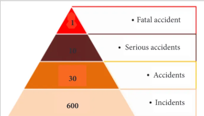
Figure 1, known as 1:600 Rule, is the result of a research in the industrial environment in 1969 and illustrates the average percentage ratio between incidents and accidents (Bird and Germain, 1969 apud ICAO, 2005).
Figure 1 shows that small events occur at a greater frequency than accidents and its severity is inversely proportional to the possibility of occurrence. However, a major risk factor is that the majority of incidents are not reported. Thus, small incidents that were not considered can become events that, by their turn, might trigger a serious accident.
herefore, there is a critical aspect of human factors which includes the manufacture of the avionics system, its installation, operation and maintenance, and that depends on the personnel involved in reporting problems or faults. his is not always eicient. With respect to the human factors involved, safety barriers can be created if critical parameters of the installation of each system are analyzed and procedures to reduce the unsafe conditions are elaborated.
INSTALLATION AND MAINTENANCE OF AVIONICS SYSTEMS THROUGH REPAIR STATIONS, SERVICE CENTERS AND OTHER MAINTENANCE FACILITIES IN BRAZIL
he variety of failures that may occur in the components of avionics equipment, combined with the diversity of aircrat manufacturers and suppliers, may make the categorization of unsafe situations impossible by an analysis method of internal components and their interconnections, for the existing range of avionics systems.
Except for the case of an aircrat repair, the avionics systems installation usually occurs in two ways: through direct incorporation of the aircrat’s type design or by major type design change. he avionics incorporated into the project type are made by the manufacturers of the aircrat or under their supervision. However, in Brazil, the most common way to install avionics is through major changes at installer’s facilities. hus, the unsafe factors for avionics systems are closely related, besides the manufacturing, installation and maintenance. he maintenance and installation stations have a vast knowledge of unsafe factors in the ield and, in addition to the aircrat’s pilots, are the initial point that reports problems to manufacturers.
On one hand, some low complexity aeronautical systems, properly approved, may be developed by Brazilian facilities,
Figure 1. 1:600 Rule.
Fatal accident
Serious accidents
Accidents
Incidents
10
30
600 1
such as: LED lighting systems, power supplies, small control panels and supports etc. On the other hand, when an aeronautical facility are installing an avionics system that was not developed by its own means, this one does not have access to all the design parameters, being unaware of hardware and sotware details of the system. Consequently, various tests must be performed in a device in order to be certiied for aviation usage.
Another relevant factor is the current use of Integrated Modular Avionics (IMA). With IMA, the maintenance of avionics systems is basically performed by modules substitution or by the replacement of the whole equipment, which are then sent (the IMA or complete equipment) to their respective manufacturers. Probably, the Brazilian installers do not have the necessary conditions to execute the kind of repair that is performed by the IMA system manufacturer. hus, for a case study on maintenance of avionics in Brazil, an emphasis on systems should be adopted, avoiding a deep approach on component failures, because it is likely that most Brazilian facilities will not have access to failures analysis of IMA components.
APPROVAL OF MAJOR MODIFICATIONS TO INSTALL AVIONICS SYSTEMS IN BRAZIL
he PST group – Supplemental Type Program (Grupo PST – Programa Suplementar de Tipo) that belongs to Aeronautical Products Certiication Branch (GGCP – Gerência-Geral de Certiicação de Produto Aeronáutico) of SAR/ANAC is responsible for major changes certiication in Brazilian registered aircrat, including the installation of avionics systems. he PST group has a database of public domain, which lists the major changes certiied in Brazil, from where the data used in this work was collected.
TAWS – TERRAIN AWARENESS AND WARNING SYSTEM
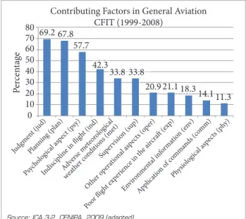
For years, Controlled Flight Into or Toward Terrain (CFIT) category of accidents, dominated the global statistics of accidents. As deined by the ICAO/CAST (2011), CFIT is a collision in light or near collision with terrain, water or obstacle without indication of loss of control. Figure 2 shows the causes of CFIT for General Aviation in Brazil, between 1999 and 2008, according to CENIPA.
Following the recommendations of ICAO for CFIT prevention, Brazilian regulations RBAC/RBHA 91, 135 and 121 establish requirements for the installation of Ground Proximity Warning System (GPWS) in the aircrat.
An enhanced version of the GPWS System is called Terrain Awareness and Warning System (TAWS), which uses geo-location systems like Global Navigation Satellite System (GNSS) and databases that include terrain and a large amount of man-made obstacles to generate alarms and alerts. he installation of TAWS and GPWS has contributed to a substantial reduction in the number of CFIT accidents.
here are two classes of TAWS systems: class A TAWS, which has interconnection with a display, radio altimeter and/or air data computer, and class B TAWS, where the interconnection with a display is not mandatory. Figure 3 illustrates a typical class A TAWS system, with some of its main common components, such as altimetry and positioning inputs, data processor, display and visual and aural alerts.
From direct observation of the data presented in the public database of modiications, the PST group analyzed data of the certiication processes during the year 2009 and concluded that the TAWS/GNSS installations accounted for about 50% of the total number of modiications corresponding to approximately 80% of the cases of major changes in electrical and electronic systems, presented to be certiied by ANAC. Due to these characteristics, it has been gathered a signiicant quantity of risk factors for this type of system.
In addition to this analysis, samples of processes for installations of TAWS/GNSS systems were collected from two base years: 2005, with 313 samples; and 2009, with 378 samples. hese base years were chosen because they show the two extremes of the development of this kind of installations: a pioneering phase, where there is a clear need for training of certifying companies — applicants,
Contributing Factors in General Aviation CFIT (1999-2008) 80 70 60 50 40 30 20 10 0 P er cen ta ge 69.2 67.8 57.7 42.3 33.8 33.8
20.9 21.1 18.3
11.3 14.1
Judg men
t (jud)
Plannin g (p
lan)
Psych olog
ical a spec
t (psy)
Indi sciplin
e in flig ht (in d) Envir onm enta l inf orm atio n (en v) Applic atio
n of co mm
ands (co mm) Adver se m eteo rolog ical weat her co nditio ns (m et) Super visio n (s up) Oth er o pera tiona
l asp ects (o
per)
Physio logic
al asp ects (p
hy)
Poor flig ht exp
erien ce in t
he a ircra
ft (exp)
Figure 2. Contributing Factors in General Aviation – CFIT.
installation and maintenance facilities; and a maturation phase with some degree of experience of applicants and maintenance facilities. Furthermore, in these years, other researches were conducted, such as the observations on the meteorological adverse conditions. Although the years between 2005 and 2009 could also provide sample data, these data were not measured with all the examined characteristics, therefore they were not included in this analysis. Consequently, the application of the proposed method observe only the sampled data of 2005 and 2009, as it was the initial objective of this research, that is to verify the processes in relation to risk factors, climatic factors, the systems involved and the quantity of these systems. he main risk factors detected for TAWS/GNSS systems are listed in Table 3.
MATHEMATICAL MODELING OF
RISK MATRIX, SCHELL AND SOM
PRINCIPLES OF RISK ANALYSIS AND RISK MATRIX According to Greenwell and Knight (2003), the risk can be defined as the probability of an event to occur, multiplied by the anticipated cost derived from the occurrence of the event. Equation 1 models the total risk based on this definition. In this work, the cost is considered equivalent to an indirect measure of severity (consequence) of an accident.
R=P·C (1)
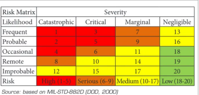
where R = total risk; P = probability; C = (cost) = severity. Basically, two criteria classify a risk: the likelihood and the severity. A risk matrix is a graphic arrangement of the risk. he origin of the risk matrix comes from the deinitions contained in MIL-STD-882D (Department of Defense – DOD, 2000). Consequently, the risk matrix is a combination of likelihood
and severity in order to classify the diferent levels of risk. Figure 4 illustrates an example of risk matrix.
he Risk Matrix is usually employed in civil and military applications, because it is an easy method used in risk management; but this method has some inherent limitations, as identiied by Cox (2008). hese are: low resolution, error induction, ineicient reallocation of resources based on the categories provided in the matrix, and ambiguity of inputs and outputs.
APPLICATION OF THE SCHELL MODEL INTERFACES
As seen in Fig. 2, the inluence of human factors is preponderant over the other CFIT factors. Due to this, the SCHELL method for human factors was adapted for the IMFLAR method in order to analyze inluence of human factors during the certiication process. hese inluences are employed as IMFLAR input parameters into a reliability model for the analysis of the involved risk in an avionics system installation during a certain period of time.
As previously described in this work, the preliminary SHEL model (Edwards, 1972), which was developed to analyze the human factors interfaces, was modiied to include other additional interfaces. Itoh et al. (2004) use the concept of m-SHEL model from Kawano (Itoh et al., 2004 apud Kawano, 2002) in a table format, grouping the interfaces in pairs. A practical application of this format, adapted from the work of Itoh et al. (2004), is presented in the item 3 – “SCHELL indexes block” of section“IMFLAR Method”, where the interfaces used are: LC – cultural interface; LS – sotware interface; LH – hardware interface; LE – environmental interface; LL – interface of human relationships; L – the human element itself, such as the pilot, the certiication expert, or the maintenance technician.
SOM – SELF-ORGANIZING MAPS
A Self-Organizing Map, also known as SOM neural network, consists of just a few to even thousands of artiicial
Sensors
- ADC
- Barometric altitude - Radio altimeter
GPS Antenna
Processor
Display
Aural & Visual Alerts
TERRAIN
Sensors
- ADC
- Barometric altitude - Radio altimeter
GPS Antenna
Processor
Display
Aural & Visual Alerts
TERRAIN
Figure 3. Class A TAWS – block diagram.
Source: based on MIL-STD-882D (DOD, 2000) Figure 4. Risk matrix.
Risk Matrix Severity
Likelihood Catastrophic Critical Marginal Negligible
Frequent 1 3 7 13
Probable 2 5 9 16
Occasional 4 6 11 18
Remote 8 10 14 19
neurons organized in a grid, or lattice, usually bi-dimensional. For a competitive process of learning, the winning neurons are organized in a topographic map, as in the areas of the human brain. his map is a statistical arrangement in terms of the inputs (Castro and Castro, 2001).
he mathematical deinition of SOM requires the deinition of Euclidean vector. For an input signal x(t) as Euclidean vector of d dimension (Kohonen and Honkela, 2007) is deined according to Eq. 2:
x(t)=[ξ1 (t),ξ2 (t), ξ3 (t), .... , ξd (t)] (2)
where: x(t) = Euclidean input vector, consisting of d input signals; t = data index in a sequence; ξ(t) = input signals; d = dimension, or quantity of input signals.
Each neuron of the SOM network is represented by a weight vector, according to Eq. 3:
m = [m1, m2, m3, ..., md] (3)
where: m=d-dimensional weight vector; d is the dimension of the input vector.
he neurons of the network represent the input vectors in the best possible way. Each input vector is presented to all neurons of the network and the “winner” is the one with the closest weight, i.e., the neuron with more similarities to the input vector in question. In this work, the Euclidean distance is used to determine the “degree of similarity” between the input vector and weights of the neurons. he “winner” neuron c for an input vector x is the one that has its weight value m with the smallest Euclidean distance to the input vector x. he winner neuron is also called the Best Match Unit (BMU), around which the closer neurons are organized. he organization of neurons is a process of smoothing by similarity, deined by the function called Nc –neighborhood of the winner. Ater inding the BMU, the network is updated by an iterative process (adapted from Laurino, 2004; Kohonen and Honkela, 2007).
According to Reyes-Aldasoro (1998), the process of neurons self-organization (called nodes of the grid) on a SOM network can be described in two steps: combination of inputs and neurons; and updating around winning neurons. hese processes are modeled by Eq. 4 and Eq. 5:
Combination:
x(t) = || x(t)-mc (t) ||= mini|| x(t)-mini(t)|| (4)
Updating:
[ ]
= +
∈
-+
= +
c i
i
c i
i i
N i t m t
m
N i t m t x t t m t
m
), ( ) 1 (
, ) ( ) ( ) ( ) ( ) 1
( ∝
⎨ ⎧
⎩ ∉
(5)
where, for a time t: x = input; mi = any node; mc = winner neuron; α = sequence of gain; and Nc = neighborhood of the winner neuron (in this work, Nc is deined internally in the sotware utilized). Each neuron is connected to adjacent neurons by the neighborhood relation Nc, which determines the topology of the SOM map. The topology has two attributes: structure and shape (Vesanto et al., 2000). Figure 5 shows the structure and shape for the SOM network used in this work.
Grouped neurons can also be presented in other graphic format, known as U-matrix (Vesanto et al., 2000 apud Francisco, 2004). A U-matrix shows, through the colored units of the map, the distances between clusters. he colors of a U-matrix vary according to a distance scale, from dark blue to red, where the dark blue color represents the 66 nearest cells (neurons), or groups. he lighter colors to red represent the separation of the clusters (according to Vesanto et al., 2000 apud Francisco, 2004). Figure 6 shows an example of a U-matrix, applying the data to be presented in this work to a SOM network through the tool SOM_TOOLBOX_2, for MATLAB®
. his toolbox is shortly described in step 4 of IMFLAR.
Figure 5. SOM topology: hexagonal structure grid and plane shape.
6.74
3.6
0.47
IMFLAR METHOD
IMFLAR DESCRIPTION
IMFLAR: An Intuitive Method for Logical Avionics Reliability is a method that organizes data from the PST public database, combining them with CFIT accidents statistical data, taking into account the interfaces from the SCHELL model. hese weighted data are grouped by a SOM neural network that organizes them into risk groups. hese groups and the organized SCHELL data are then used for the development of a simulation model in Simulink/ MATLAB®
. his reliability model of can predict a situation of increased risk based solely on the data presented, modeling human factors, environmental and machine involved with the installation of the avionics system under analysis.
he IMFLAR overcomes each of the limitations of Risk Matrix, due to the lexibility of the SOM neural network employed and its presentation in graphical format.
As an application of the proposed method, the installations of TAWS avionics in Brazil are analyzed through a Safety Assessment analysis. his proposed analysis exempliies the relationship between a statistical data from an accidents category (CFIT) and the installation of an avionics system that prevents this kind of accident.
An alteration of risk, during the operational life of the aircrat, with the modiication that installs the avionics system under analysis can be simulated by a variation of a source block parameters in the model in the Simulink/MATLAB® presented. hus, the IMFLAR method can simulate the risk variation during the course of the years for an avionics system. An application of this simulation can be the creation of an alternative solution to generate other maintenance tasks for the system under analysis.
he following subsections present: the steps that show how to acquire data for the IMFLAR; and the procedures for the elaboration of a simulation model on Simulink/MATLAB®
.
STEPS OF IMFLAR – ACQUIRING DATA
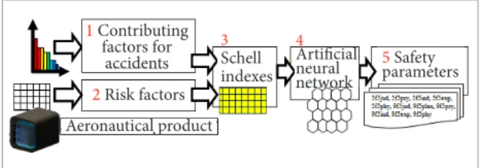
Figure 7 shows a block diagram that describes the necessary steps to implement the proposed method. Each block is described by its input, processing of data by the block, and its output.
Step 1 – the block of contributing factors for accidents
• Input item: equivalent to the statistical causes of real accidents related to the conditions of use of the certiied system. his paper uses the statistical data of the major
causes of CFIT in General Aviation - 1999 to 2008, according to the CENIPA data records (CENIPA, 2009). • Data processing item: these statistics of the CFIT causes
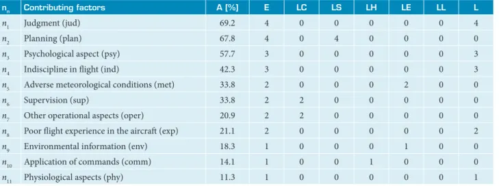
are scaled by the percentage of occurrence, according to Table 1, resulting in ive risk levels (named E - Exposure). he scaling reproduces the way levels of the risk matrix are elaborated. he proposed scaling is just an example and other subdivisions are also possible. However, for a smaller number of divisions, the method tends to be less accurate, and for the higher number of subdivisions, the number of parameters to be analyzed tends to be greater. he Level or Amplitude is deined as the amount, in percentage, of installations involved with the risk factors, and the Exposure means the exposure to risk. Table 1 shows the relationship between the Exposure (E) and the Level or Amplitude (A).
Indexes A and E are determined by the application of Table 1 to the 11 contributing factors determined by the CENIPA, according to Fig. 2. For example, for the irst contributing factor <Judgment (jud)>, corresponding to the Level or Amplitude A=69.2%, then 26% <A≤80%, which corresponds, according to Table 1, to an Exposure E=4. • Output item: as output of this block, the initial four
columns of Table 2 enumerate and present the 11 contributing factors described by the CENIPA, and show the respective indexes A and E for these factors, which are the inputs to the SCHELL indexes block, described by the other columns of Table 2. he SCHELL indexes block is presented in step 3.
Step 2 – the risk factors block
he IMFLAR introduces a new concept in the certiication of an aeronautical system: generic unsafe conditions, observed during the certiication process of major change that installs this system, are considered as parameters to be analyzed, which may cause future risk events, ater installation and during the operation of this system.
1 Contributing factors for
accidents
2 Risk factors
Aeronautical product 3 Schell indexes
4 Artificial neural network
5 Safety parameters 1 Contributing
factors for accidents
2 Risk factors
Aeronautical product 3 Schell indexes
4 Artificial neural network
5 Safety parameters 1 Contributing
factors for accidents
2 Risk factors
Aeronautical product 3 Schell indexes
4 Artificial neural network
5 Safety parameters
• Input item: inputs of this block are the unsafe conditions, obtained from a sample of certiication procedures relating base years of 2005 and 2009, for the TAWS system. he TAWS system was chosen because of the greater amount of processes for modifying aircrat relative to other systems. It was observed in the initial introduction of this system in Brazil (2005) and in a more advanced stage (2009), corresponding to a period in which the applicants for modiication processes achieved a stage of maturation of the presented projects. he main risk factors detected for TAWS/GNSS systems are presented according to Table 3.
• Data processing item: the same scaling process adopted for the block of contributing factors for accidents. For example, if the training factor corresponded to a Level A=100% of afected processes in the base year of 2005, this implies an Exposure E=5.
• Output item: Table 4 presents the indexes A and E for risk factors as inputs to the SCHELL indexes block. As the output of this block, the initial three columns of Table 4 enumerate the 11 contributing factors, as described by
the CENIPA as fm (m = 1-11) and present the indexes A and E for these factors, which are inputs to the SCHELL indexes block, described by the other columns of Table 2. he SCHELL indexes block is presented below.
Step 3 – The SCHELL indexes block
• Inputs items: are the outputs of the previous two blocks, namely, contributing factors for accidents and risk factors, corresponding to the Exposure E in Tables 2 and 4.
• Data processing item: as observed on the CENIPA statistics and in other studies of accidents, the inluence of human factors is predominant over other risk factors of an accident. herefore, the exposures E of Tables 2 and 4 are combined by the SCHELL method of interfaces based on human factors. For this work, these interfaces are named SCHELL indexes. he presentation of the interfaces, in table format, uses a concept similar to m-SHEL model of Kawano (2002) adapted from SCHELL model. his model works, therefore, with six interfaces: LC, LS, LH, LS, LL, L, where L is the irst inluence of the human factor (pilot). he other factors of these interfaces are: LC – human /cultural interface, for example, supervision (air traic control) or training; LS – human/ procedure interface, for example, planning; LH – man/machine interface, for example, the application of controls; LE – human/ environment interface, for example, environmental conditions; LL – man/man interface, for example, interaction between pilots; L – man, that is, the pilot and his own condition, for example, lack of experience of the pilot in the aircrat. hese indexes are weighted as follows:
Table 1. Relationship between Exposure (E) and Level or Range (A).
E A [%]
1 A≤20
2 20<A≤40
3 40<A≤60
4 60<A≤80
5 A<80
Table 2. Contributing factors to CFIT in general aviation (1999-2008) and SCHELL indexes.
nn Contributing factors A [%] E LC LS LH LE LL L
n1 Judgment (jud) 69.2 4 0 0 0 0 0 4
n2 Planning (plan) 67.8 4 0 4 0 0 0 0
n3 Psychological aspect (psy) 57.7 3 0 0 0 0 0 3
n4 Indiscipline in light (ind) 42.3 3 0 0 0 0 0 3
n5 Adverse meteorological conditions (met) 33.8 2 0 0 0 2 0 0
n6 Supervision (sup) 33.8 2 2 0 0 0 0 0
n7 Other operational aspects (oper) 20.9 2 2 0 0 0 0 0
n8 Poor light experience in the aircrat (exp) 21.1 2 0 0 0 0 0 2
n9 Environmental information (env) 18.3 1 0 0 0 1 0 0
n10 Application of commands (comm) 14.1 1 0 0 1 0 0 0
n11 Physiological aspects (phy) 11.3 1 0 0 0 0 0 1
(A) Each of the contributing factors of accidents in Table 2 is analyzed. For example, the factor n1 Judgment (Jud), E=4. For each factor, only one SCHELL index is chosen as predominant to avoid problems with the possible ambiguity of data in order to make the neural network grouping of data in a more eicient way. For the Jud factor, the L index was chosen. hen, the same value of E for L is assigned, therefore, L=4. For other factors, the weight is zero, so LC=LS=LH=LE=LL=0. In this case, the same analysis is also repeated for the other factors.
(B) Similarly, each risk factor in Table 4 is analyzed. For example, for the factor f1 Weather of 2005, E=1. For the Jud Factor, the LE index was chosen. hen, the same value of E is assigned to LE, therefore LE=1. he weight of other factors
are set to zero, i.e., LC=LS=LH=LL=L=0. In this case, the same analysis is also repeated for the other factors.
(C) he predominant indexes in Table 2 are multiplied by the predominant indexes of Table 4, as shown in Fig. 8, in order to obtain Table 5.
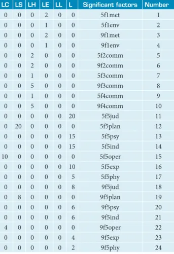
(D) For Table 5 preparation, according to the previous procedure, ten auxiliary tables are generated (five tables for five risk factors in 2005, and five tables for five risk factors in 2009). Each table has 11 rows, referring to the contributing factors, and 6 columns, related to SCHELL indexes, totalizing 66 elements. Most of the rows of the auxiliary tables contain only zeros, and only the 24 remaining lines contain significant elements that were grouped in Table 5.
• Output item: the output of the SCHELL indexes block is composed of the significant factors that are presented to the neural network SOM of the artificial neural network block. After the development of Table 5, it is verified that only 24 factors are considered significant. These significant factors, in a practical approach, represent the Vulnerability of the system. Vulnerability is defined, in this paper, as a potential factor in exposing the analyzed system to the risk of an aircraft incident or accident. Therefore, the function of the SCHELL indexes block is similar to a Vulnerability detector, according to this definition.
Table 3. Survey of risk factors for TAWS Systems in 2005 and 2009.
Factor number Element Quality for analysis Unit Base year
2005 2009
factor number Process Total of processes Total of processes [units] 313 378 f1 Weather Inluence of weather during the year Percentage of cases [%] 2.75 2.00 f2 Antenna Installation in pressurized aircrat Percentage of cases [%] <20 28.2
f3 Processor Sotware update Unit per system [pcs./System]
Percentage of cases [%]
0 0
1
f4 Display Erroneous data Unit per system [pcs./System]
Percentage of cases [%]
0 0
2
f5 Training Insuicient training Need of training [units] -1
Percentage of cases [%]
1 100
1/4 25 Source: ANAC/PST
Data were obtained from two base years: 2005 with 313 cases sampled, and 2009 with 378 cases sampled, with the analysis of the following aspects:
1 – Weather factor: indicates the percentage of processes that were, somehow, affected in the base year due to meteorological conditions. These data were obtained, indirectly, from the public database of processes of the PST, through the records of cancellations of inspections/tests and comparison with the weather on the date/place of inspection/test. 2 - Antenna factor: indicates the percentage of processes that were, somehow, structurally affected due to the installation of antennas in pressurized aircraft. These data were obtained, indirectly, from the public database of processes of the PST, through the records of processes of the prototype aircraft, which were pressurized.
3 - Processor factor: indicates the quantity per unit of TAWS equipment for each system affected by software update (“load”). These data were obtained directly from the quantity of TAWS equipment to be installed in the process, which is affected by the software update (“load”), per manufacturer’s service bulletin. 4 - Display factor: indicates the quantity per unit of TAWS equipment for each system affected by the presentation of erroneous data. These data were obtained directly from the quantity of TAWS equipment to be installed in the process, which is affected by the manufacturer’s service bulletin that corrects this erroneous data. 5 - Training factor: measures the variation of the learning curve regarding to the installation/operation of the system. This factor was obtained indirectly by the number of meetings proposed by the modiication process applicants, where it was observed that the value of the number of meetings (f5) decreased, in absolute value, inversely proportional to the elapsed time (t) according to: f5≅a | t-1 | where: f5 = number of meetings per year ≅ need of annual training; α = index for units comparison - where, to the research data: α = α [s. (units / year)]; t = elapsed time
(it was considered an average time of four years between the second half of 2005 and the irst half of 2009).
Table 4. Risk factors and SCHELL indexes.
Factor per year (2005) A [%] E LC LS LH LE LL L
f1 Weather 2.75 1 0 0 0 1 0 0
f2 Antenna 20 2 0 0 2 0 0 0
f3 Processor 0 1 0 0 1 0 0 0
f4 Display 0 1 0 0 1 0 0 0
f5 Training 100 5 5 5 0 0 5 5
Factor per year (2009) A (%) E LC LS LH LE LL L
f1 Weather 2.00 1 0 0 0 1 0 0
f2 Antenna 28.2 2 0 0 2 0 0 0
f3 Processor 80 5 0 0 5 0 0 0
f4 Display 80 5 0 0 5 0 0 0
f5 Training 25 2 2 2 0 0 2 2
Step 4 – artiicial neural network block
• Input item: inputs of this block are the signiicant factors yielded from SCHELL indexes block output and correspond to the input data of the SOM neural network.
• Data processing item: in this block, the SOM tool was applied, a neural network which classifies significant factors. For this, the SOM_TOOLBOX_2 was used. This toolbox was created by the Laboratory of Computer and Information Science (CIS) of Helsinki University of Technology for MATLAB®
. The SOM_TOOLBOX_2 groups and sorts the data into a graphical format, denominated Self-Organizing Map (SOM). This toolbox consists of a series of mathematical functions and graphs, which are elaborated using the MATLAB® functions. The SOM_TOOLBOX_2 has some specific program instructions for data collection, training the network and displaying the data.
(A) he input function item: the reading of signals is performed by the instruction “som_read_data”. his function recognizes only iles with extension “.data” created by the program SOM_PACK (also developed by Helsinki University of Technology), written in C language, which has no compiler for the Windows®
platform. hus, for use in the MATLAB® running under the Windows®
, the input data must be converted to a text ile in ASCII format, as shown in Fig. 9:
(B) he combination and update functions item: once data is acquired, the SOM network is created, initialized and trained by the command “som_make” which performs combination and update functions.
(C) he output function item: data grouped by the SOM are displayed through the “som_show” function in various graphical presentations, for example, by U-matrix or cellular maps, as shown in Fig. 10.
• Output item: the output of this block is the data presented in map format by the function “som_show.” Data in Table 5 are grouped by the SOM tool, as shown in Fig. 10. This Figure also shows the corresponding U-matrix. Significant factors are, thus, grouped and mapped by the SOM neural network and these groups are named, in this work, as safety parameters. Therefore, the safety parameters are the critical design points that can imply in failures of the system under study and, in practice, are equivalent to the grouping of the system’s Vulnerabilities.
Table 5. Signiicant factors.
LC LS LH LE LL L Signiicant factors Number
0 0 0 2 0 0 5f1met 1
0 0 0 1 0 0 5f1env 2
0 0 0 2 0 0 9f1met 3
0 0 0 1 0 0 9f1env 4
0 0 2 0 0 0 5f2comm 5
0 0 2 0 0 0 9f2comm 6
0 0 1 0 0 0 5f3comm 7
0 0 5 0 0 0 9f3comm 8
0 0 1 0 0 0 5f4comm 9
0 0 5 0 0 0 9f4comm 10
0 0 0 0 0 20 5f5jud 11
0 20 0 0 0 0 5f5plan 12
0 0 0 0 0 15 5f5psy 13
0 0 0 0 0 15 5f5ind 14
10 0 0 0 0 0 5f5oper 15
0 0 0 0 0 10 5f5exp 16
0 0 0 0 0 5 5f5phy 17
0 0 0 0 0 8 9f5jud 18
0 8 0 0 0 0 9f5plan 19
0 0 0 0 0 6 9f5psy 20
0 0 0 0 0 6 9f5ind 21
4 0 0 0 0 0 9f5oper 22
0 0 0 0 0 4 9f5exp 23
0 0 0 0 0 2 9f5phy 24
The 24 parameters in Table 5 are designed as the example below:
5f1met = Relationship between the risk factor (f1) from 2005 and contributing factor n5
5 = base year of data collection (2005)
f1 = risk factor Weather (refer to Table 4) met = contributing factor to CFIT “n5” - Adverse meteorological conditions (refer to Table 2)
Table 2
Table 4
Table 5 Contributing factors
Factors per year (2005)
Significant factors 5f1met
Equal
Plus
f1 Weather
Adverse meteorological conditions (met)
nn n5
LE 2
1 LE
LE 2
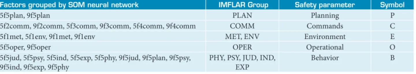
Step 5 – the safety parameters
• Input item: data grouped by SOM neural network.
• Data processing and output item: signiicant factors grouped by neural network are organized in Table 6. his grouping is essential to an engineering analysis of these parameters, because the signiicant factors are grouped into common areas. At the same time, the study by areas decreases the number of parameters to be examined. his reduces the cost of man-hour analysis of which parameters signiicantly afect project’s safety.
The procedures for elaboration of simulation model
on Simulink/MATLAB®
1. he determination of the risk variation per time
Figure 11 shows pairs of signiicant factors from Table 5 used as the boundaries of variation of the involved risk. his risk represents the workload for pilot, actions for operational/ certiication team from aviation authority, veriications for continuous airworthiness and periodic maintenance tasks, or other parameters to be investigated as appropriate.
Each IMFLAR Group B, P, O, C and E is representative of the involved risk for the analyzed system (GPS/TAWS). he risk is composed by the sum of parcels of IMFLAR Group elements and each IMFLAR Group adds a combination of the Eq. 6 and Eq. 7 as applicable. hese equations are itting the values of the T, in order to combine them with the maximum values of each signiicant factor from Table 5.
un=anT+bn (6)
vn=cnT+dn (7)
where: T = time variation; an; bn; cn; and dn = adjustable values, in order to it the equation with the extremes values of signiicant factors from the Table 5; and un, vn = risk variation per time (unandvnare diferent functions which variations are related with the IMFLAR Group as demonstrated as follow).
Example for calculation of anandbn for u7: From Eq. 6: un=anT+bn⇒ u7=a7T+b7;
From Table 5:
t=1(2005)⇒T7 = (t/100) = (1/100) and u7=5f5comm =10; t=5(2009)⇒T7 = (5/100) = (1/20) and u7=9f5comm=4.
The values of (T7, u7)2005 and (T7, u7)2009 are used to solve the equation u7=a7T+b7, in order to obtain the values of a7 andb7.
he variable T shows the behavior of involved risk (represented by IMFLAR Groups) per elapsed time. hus, the involved risk has three diferent functions per time
Table 6. Safety parameters and IMFLAR groups.
Factors grouped by SOM neural network IMFLAR Group Safety parameter Symbol
5f5plan, 9f5plan PLAN Planning P
5f2comm, 9f2comm, 5f3comm, 9f3comm, 5f4comm, 9f4comm COMM Commands C
5f1met, 5f1env, 9f1met, 9f1env MET, ENV Environment E
5f5oper, 9f5oper OPER Operational O
5f5jud, 5f5psy, 5f5ind, 5f5exp, 5f5phy, 9f5jud, 9f5plan, 9f5psy, 9f5ind, 9f5exp, 9f5phy
PHY, PSY, JUD, IND, EXP
Behavior B
Figure 9. Example of SCHELL signiicant factors (P1 to Pn, n=1 to 24) for the analysis of the SOM network.
SL
0.00.0
...
...
...
...
...
... ...
0.0 0.0 0.0 0.0 0.0 0.0 0.0 0.0 0.0 0.0 P1Pn
CL HL EL LL
L
U-matrix 6.7
3.6
0.4
Labels
20
15
10
5
0
5f1m
et
9f1m
et
5f1ef
v
9f1ef
v
5f2co
mm
9f2co
mm
5f3co
mm
9f3co
mm
5f4co
mm
9f4co
mm
5f5o
p
er
9f5o
p
er
5f5p
la
n
9f2p
la
n
5f5j
ud
9f5j
ud
5f5psy 9f5psy 5f5in
d
9f5in
d
5f5exp 9f5exp 5f5p
h
y
9f5p
h
y
Figure 11. Signiicant factors.
depending on the analyzed group. It is not dependent on human factors in Group E (the extremes are matching = constant function). It is composed by a constant function and an increasing function for group C and the risk is decreasing for groups B, P and O.
(A) IMFLAR Groups B, P, and O have a directly relationship with human factors and the Training factor from Table 3 and, for this case, the Eq. 6 is fitted by Eq. 8. This represents the “man” interactions or “human factors” influence.
Table 7. IMFLAR application.
Function
un=anT+bn
T=100/=f5 with a=100 (100%)
Group un Factor an bn fn
B u1 phy 3/80 5/4 f5=T=100/t
B u2 exp 3/40 5/2 f5=T=100/t
B u3 ind 9/80 15/4 f5=T=100/t
B u4 psy 9/80 15/4 f5=T=100/t Risk per time
B u5 jud 3/20 5 f5=T=100/t B=u1+u2+u3+u4+u5
P u6 plan 3/20 5 f5=T=100/t P=u6
O u7 oper 3/40 5/2 f5=T=100/t O=u7
Function
vn=cnT+dn T=t
Group vn Factor cn dn fn
C v1 f2comm 0 1 f2=1
C v2 f3comm 1 0 f3=t Risk per time
C v3 f5comm 1 0 f4=t C=v1+v2+v3=f2+ f3+f4=2t+1
E v4 f1met -0.01168 0.9168 v4=2f1/100 Risk per time
E v5 f1env -0.00584 0.4584 v5=f1/100 =(-0.548t+45.84)/100 E=v4+v5=2f1+f1=3f1
(B) For the IMFLAR Group C the involved risk are rising with time (this is an accumulative risk which represents the software loads, deterioration of components and others aspects related to the maintenance and continuous airworthiness of system). This function was considered linear for an initial approach. This represents the “machine” factor.
(C) For IMFLAR Group E, the acquired values of met=2*env (constants for the collected data) are replaced by the average curve (f1=-0.548t+45.84) that represents the “seasonal variability of rainfall in the São José dos Campos airport fields between the years 1982 and 2009”, according Corrêa et al. (2010). he site of São José dos Campos was elected because it represents the local were the most certiication tests were performed for GPS/TAWS systems related to this research. he function f1 were divided by100. his is necessary for adjusting the magnitude of the variables to a reasonable value of IMFLAR Group E. his represents the “environment” factor.
he same procedure for calculation of an andbn for u7 can be utilized for the determination of other un andvn values. hese calculations are summarized in Tables 7 and 8.
2. he elaboration of the Simulink/MATLAB®
Figure 12 presents a Simulink/MATLAB®
model that represents the elements of Tables 2 to 8 for the IMFLAR. he equations that model the blocks are on Table 8 and the elements of this model are on Tables 2 to 8. his model translates the representation of IMFLAR parameters to a functional block diagram in order to simulate and foresee the variation of risk per time, including a separated analysis for “human factors”, “machine” and “environment” inluences as previously explained.
Figure 13 presents a graphical representation of IMFLAR Groups variations and the resulting risk R for the IMFLAR.
Table 8. Summarization of equations from Table 7.
Function Description Function number
un=anT+bn Fit function of T=100/t from the Eq. 8 (9)
vn=cnT+dn Fit function of T=t (10)
f1=-0.548t+45.84 Function for factor per year =f1 (11)
f2=1 Function for factor per year =f2 (12)
f3=t Function for factor per year =f3 (13)
f4=t Function for factor per year =f4 (14)
T for Eq. (9) → f5=T=100/t Time variation (T) and function for factor per year =f5 (15)
T for Eq. (10) → T=t Time variation (T) (15)
B=u1+u2+u3+u4+u5 Risk per time for B group (16)
P=u6 Risk per time for P group (17)
O=u7 Risk per time for O group (18)
C=v1+v2+v3=f2+ f3+f4=2t+1 Risk per time for C group (19)
E=v4+v5=2f1+f1=3f1 Risk per time for E group (20)
3. A practical application of Simulink/MATLAB®
model for IMFLAR
With the elaborated model, it is possible to test an individual parameter variation. Figure 14 represents the behavior of R related to a variation (step) on the O group signal. his variation is implemented by the block arrangement illustrated in Figure 14 and it might characterize an operational change. An example of this change could be the introduction of new rules for aviation in order to comply with the phases for Performance-Based Navigation (PBN) implementation in Brazil. his is a versatility example of the proposed IMFLAR.
CONCLUSIONS
he growing of the General Aviation leet and the development of new avionics systems demand needs to increase light safety, which is aeronautical authorities’ responsibility in partnership with manufacturers, maintenance teams and other aviation professionals. To do this, it may be necessary to develop other Safety Assessment methods using more adequate approaches to new patterns. hus, an artiicial neural network can be a viable alternative, since its efectiveness is appropriately certiied.
he proposed IMFLAR, on the SOM artiicial neural networks, enables simulating logical decisions and groupings, similar to the human brain. he grouping of unsafe parameters turns the application of this presented method into a practical tool for an avionics system installation project. he grouping of these parameters is also one of the main advantages of the proposed method over other project methods, mainly because the safety parameters grouped by SOM are general and do not have a direct relation to unsafe conditions for any speciic equipment from any manufacturer, but these parameters relate common failures of any functionality. hus, it can be used to verify the vulnerabilities of a functionality, such as TAWS, which can be commercially supplied by various equipment, or may be present in future systems to be designed. hus, this method can also be predictive and may be used to foresee safety parameters, vulnerable areas of functionalities in future systems or simulate an unsafe operational condition as described in this work.
Figure 14. Simulink/MATLAB® model outputs – operational variation.
0 0 5 10 20 25
15
2 4 6 8 10 12 14 16 18 20 Time (years)
U
n
sa
fet
y F
ac
to
r
O R
0 5 10 20 25
15
2 4 6 8 10 12 14 16 18 20
Time (years)
U
n
sa
fet
y F
ac
to
r
B P O C E R
Figure 13. Simulink/MATLAB® model – IMFLAR groups and risk outputs.
Likewise, on any computational method used for Safety Assessment, an engineering analysis of the data grouped by SOM is necessary, in order to avoid errors. However, as described in this article, the application of this method is simple, the graphical grouping is easy to understand, and the presented results allows one to conclude that this method can be employed, not only as a Safety Assessment tool, but as an application for a predictive design where unsafe conditions are described by equations that are translated into the blocks of the simulation model and any safety parameters variation can be tested.
Finally, the proposed IMFLAR can be considered an upgrade of other established methods, such as the Risk Matrix and the SCHELL model, overcoming some limitations of these methods and proposing new approaches to Safety Assessment and predictive design, showing potential of using this method for aeronautical applications and other engineering areas.
ACKNOWLEDGMENT AND
DISCLAIMER
he authors would like to thank the support of experts from the National Civil Aviation Agency – ANAC and Aeronautics Institute of Technology – ITA, in preparing this article.
REFERENCES
Aircraft Crashes Record Ofice (ACRO), 2011, “Various Statistics”, retrieved in 17 Aug. 2011, from http://www.baaa-acro.com/ Statistiques%20diverses.html.
Aircraft Owners and Pilots Association (AOPA), 2010, “AOPA General Aviation Trends Report”, Fourth Quarter 2010, AOPA Online, retrieved in 17 Aug. 2011, from http://www.aopa.org/whatsnew/trend.html.
Agência Nacional de Aviação Civil (ANAC), “Aircraft Modiication – Brazilian STC (CHST)”, PST/GGCP/SAR/ANAC, retrieved in 17 Aug. 2011, from http://www2.anac.gov.br/certiicacao/CHST/CHSTE.asp
Agência Nacional de Aviação Civil (ANAC), “Control of Supplemental Type Certiication Processes”, PST/GGCP/SAR/ANAC, retrieved in 17 Aug. 2011, from http://www.anac.gov.br/certiicacao/PST/ index_pst.asp
Associação Brasileira de Aviação Geral (ABAG), 2011, “Anuário Brasileiro de Aviação Geral – 2011”, Brazil.
Bird, F.E. Jr. and Germain, G.L., 1969, “Damage Control”, American Management Association, New York, 1969.
Braga, P.L., 2006, “Reconhecimento de voz dependente de locutor utilizando Redes Neurais Artiiciais”. Escola Politécnica de Pernambuco. Universidade de Pernambuco, PE, Brazil.
Burin, J.M., 2011, “Leveling off”, Aerosafetyworld, Flight Safety Foundation, Feb. 2011.
Castro, F.C.C. and Castro.M., 2001, “Mapas de Kohonen (Self-Organizing Map). Redes neurais artiiciais”, dissertação de mestrado, Pontifícia Universidade Católica do Rio Grande do Sul (PUCRS), Cap. 7, RS, Brazil.
Centro de Investigação e Prevenção de Acidentes Aeronáuticos (CENIPA), 2009, Instrução do Comando da Aeronáutica. ICA 3-2. “Programa de prevenção de acidentes aeronáuticos da aviação civil brasileira para 2009”.
Corrêa, C.S., Villaron, M.A., Araujo, R.T. and Pinto, M.L.A., 2010, “Variabilidade sazonal da precipitação no aeroporto de São José dos Campos – SP entre os anos de 1982 e 2009”, IN: CONGRESSO BRASILEIRO DE METEOROLOGIA, XVI., 2010, Belém. Anais do XVI CBMET, Belém, PA, Sociedade Brasileira de Meteorologia (SBMET), 2010. retrieved in 12 Sep. 2012, from http://www.cbmet2010. com/anais/artigos/310_40078.pdf.
Cox, A.L., 2008, “What’s Wrong with Risk Matrices?”. Risk Analysis, 28 (2), 497-512.
Department of Defense (DOD), 2000, “Standard Practice for System Safety, MIL-STD-882D, USA.
Edwards, E., 1972, “Man and machine: Systems for safety”, Proceedings of British Airline Pilots Associations Technical Symposium, British Airline Pilots Associations, London, pp. 21-36.
Everdij, M.H.C., Blom, H.A.P. and Kirwan, B., 2006, “Development of a structured database of safety methods”, 8th International Conference on Probabilistic Safety Assessment and management (PSAM8), New Orleans, Louisiana, USA.
Federal Aviation Administration (FAA), 2010, “Developing and Implementing an Air Carrier Continuing Analysis and Surveillance System”, Advisory Circular (AC) 120-79A, U.S. Department of Transportation.
Francisco, C.A.C., 2004, “Rede de Kohonen: Uma ferramenta no estudo das relações tróicas entre as espécies de peixes” (dissertação de mestrado), Programa de Pós-Graduação em Métodos Numéricos em Engenharia, área de Concentração em Programação Matemática, Universidade Federal do Paraná, PR, Brazil.
Greenwell, W.S. and Knight, J.C., 2003, “Risk-Based Classiication of Incidents”, 2003 Workshop on the Investigation and Reporting of Incidents and Accidents.
Hawkins, H.F., 1987, “Human Factors in Flight”, Gower Technical Press Ltd.
International Civil Aviation Organization (ICAO), 2005, “ICAO Accident Prevention Programme”, ANB – Air Navigation Bureau.
International Civil Aviation Organization/Commercial Aviation Safety Team (ICAO/CAST), 2011, “CICTT Occurrence Category Deinitions”.
Itoh, H., Mitomo, N., Matsuoka, T. and Murohara, Y,, 2004, “An Extension of M-Shel Model for Analysis of Human Factors at Ship Operation”, 3rd International Conference on Collision and Grounding of Ships (ICCGS 2004), Izu, Japan.
Kawano, R., 2002, “Medical Human Factor Topics”, Saga Medical School, Saga, Japan.
Keightley, A., 2004, “Human factors study guide”, Palmerston North, Massey University, 190.216, New Zealand.
Kohonen, T., 1994, “Self Organizing Maps”, Springer Series in Information Sciences, Springer, Espoo, Finland.
Kohonen, T. and Honkela, T., 2007, “Kohonen Network”,Scholarpedia,
Vol. 2, No. 1, pp. 1568.
Laurino, L.S., 2004, “Rede Neural para classiicação de caracteres”, Instituto de Informática, PPGC – Programa de Pós-Graduação em Computação, CMP135 – Arquiteturas Especiais de Computadores, Universidade Federal do Rio Grande Do Sul, RS, Brazil.
National Transportation Safety Board (NTSB), 2010, “Introduction of Glass Cockpit Avionics into Light Aircraft”, Safety Study, NTSB/S-01/10.
Perry, M.J. and Perezgonzalez, J.D., 2010, “SCHELL model”, Page revision: 17, last edited: 22 Aug 2010, 04:55 GMT, AviationKnowledge, retrieved in 17 Aug 2011, from http://aviationknowledge.wikidot. com/aviation:schell-model.
Reyes-Aldasoro C.C., 1998, “A Non-linear Decrease Rate to Optimise the Convergence of the Kohonen Neural Network Self-Organising Algorithm”, ROCC99, Acapulco, Mexico.
SOM_TOOLBOX_2, Laboratory of Computer and Information Science (CIS) Helsinki University of Technology, retrieved in 17 Aug. 2011, from http://www.cis.hut.i/projects/somtoolbox/
Simulink/MATLAB V.7, R14/, Copyright 1984-2004, The MathWorks, Inc.
Van Der Velde, R.L., 1995, “Historical Perspective, One Hundred Years of Flight Testing”, Agardograph Agard AG, - rta.nato.int.