Abstract
The present paper aims at presenting a methodology for character-izing viscoelastic materials in time domain, taking into account the fractional Zener constitutive model and the influence of tem-perature through Williams, Landel, and Ferry’s model. To that effect, a set of points obtained experimentally through uniaxial tensile tests with different constant strain rates is considered. The approach is based on the minimization of the quadratic relative distance between the experimental stress-strain curves and the corresponding ones given by the theoretical model. In order to avoid the local minima in the process of optimization, a hybrid technique based on genetic algorithms and non-linear program-ming techniques is used. The methodology is applied in the char-acterization of two different commercial viscoelastic materials. The results indicate that the proposed methodology is effective in identifying thermorheologically simple viscoelastic materials.
Keywords
Viscoelastic materials, fractional Zener constitutive model, Mittag-Leffler function, time domain, temperature influence.
Identifying Mechanical Properties of Viscoelastic Materials
in Time Domain Using the Fractional Zener Model
1 INTRODUCTION
In recent decades, we have witnessed a huge increase in the use of polymer materials in applications within structural engineering. The good acceptance of mechanical components made from this type of material is, to a certain extent, due to the fact that they can be easily molded into basically all shapes and also to its excellent general performance in corrosive environments, and to its being a mechanical energy dissipater.
Polymers are highly viscoelastic materials (VEMs), and their mechanical properties vary greatly depending on the load application speed. This is the reason why it is important to have access to models that make it possible to predict with accuracy the mechanical behavior of this type of visco-elastic material during its life time or to predict its behavior in a wide range of frequencies.
Ana Paula Delowski Ciniello a Carlos Alberto Bavastri b Jucélio Tomás Pereira b*
a Programa de Pós-graduação em Engen-haria Mecânica, Universidade Federal do Paraná.
b Departamento de Engenharia Mecânica, Universidade Federal do Paraná, Curiti-ba, PR – Brasil.
*Author’s e-mail: [email protected]
http://dx.doi.org/10.1590/1679-78252814
The mathematical modeling of the mechanical behavior of VEMs must therefore be performed not only in frequency domain but also in time domain. Generally speaking, regarding the frequency domain approach, the idea is to impose a harmonic loading with variable frequency and known range, and use some dynamic model of the system in order to obtain the storage modulus and the loss factor in a predetermined frequency interval (Moreira et al., 2010; Martinez-Agirre and Ele-jabarrieta, 2010). Regarding time domain, the idea is to impose a stress history in order to obtain a strain history or, reversely, impose a strain history and obtain a stress history and, subsequently, apply a model of the system (Liu and Subhash, 2006; Plaseied and Fatemi, 2008; Chae et al., 2010).
One way of mathematically representing the models of linear viscoelastic behavior is through in-teger order differential equations. The main advantage of using such tool lies in its ease of storing and handling the terms, almost always trivial ones, in their derivatives and integrals. A disad-vantage is that, in order to represent the behavior of the material properly, a high number of terms is usually needed, generating a higher computational cost (Brinson and Brinson, 2008).
Another way of representing such materials is by means of models based on fractional calculus (FC). These models prove to be attractive for describing the viscoelastic behavior of many materials when added to engineering structures aiming at increasing the amount of dissipated energy (Bagley and Torvik, 1983). Models based on FC present advantages over the classical linear viscoelasticity (based on integer order derivatives) since a smaller number of terms is required for a good represen-tation of the material’s behavior – four or five parameters, for example – which, a priori, render calculation and numerical simulation easier (Pritz, 1996).
An improvement on the classical models of linear viscoelasticity may occur when replacing Newton’s viscous dampers by Scott-Blair’s fractional dampers (Mainardi, 2010). Therewith, differ-ential equations of the mechanical type written in terms of integer order derivatives are replaced by equations involving non-integer order differentiations (not necessarily of a fractional order). Among several possible models (Mainardi, 2010), the fractional Zener model (FZ) proves to be very effec-tive in predicting material behavior in a large frequency band (Pritz, 2003).
During the process of characterizing VEMs, the influence of temperature in the behavior of those materials becomes clear. In this case, a material can be defined as thermorheologically simple when all its relaxation times are affected by temperature in the same way, thus allowing the appli-cation of the Time-Temperature Superposition Principle (TTSP).
When applying the TTSP at a given temperature, the viscoelastic behavior may be associated to a behavior at another temperature through a simple shift in the time scale. Such shift allows predicting the material properties over a long period of time, from data collected in tests performed in comparatively short periods of time.
Specifically in VEMs identification processes in time domain, some works are worth mentioning. Welch et al. (1999) analyzes the quasi-static viscoelastic response of polymeric materials using consti-tutive models based on FC in time domain. The author uses fractional models of five and seven pa-rameters for the stress relaxation functions, which are capable of modeling materials in which relaxa-tion data manifest at glass level. Park (2001) characterizes a viscoelastic fluid by comparing experi-mental data to the generalized Maxwell model and to the fractional derivative model. The analysis is performed both in time and frequency domains. Jiménez et al. (2002) report a stress relaxation study in samples of PMMA and PTFE polymers (Methylmethacrylate and Polytetrafluorethylene) indicat-ing that there is not only a relaxation time, as predicted in Maxwell’s classic model, but two relaxa-tion time distriburelaxa-tions. This is approached using the fracrelaxa-tional Maxwell model. Moschen (2006) per-forms a numerical simulation of the approximate method of the inverse Laplace transform and the deconvolution method, which are used in the numerical calculation of the stress-relaxation function. The author uses the fractional standard solid model (or fractional Zener), with four parameters, ap-plied to VEMs. Pacheco (2015) presents a methodology for characterizing viscoelastic materials through an inverse problem of identification. To that end, the authors uses experimental data in time domain, extracted from stress-strain curves at different temperatures and strain rates. The methodol-ogy developed allows characterizing - in time domain - models of VEMs, based on Prony series, con-sidering the influence of temperature and pressure over the mechanical behavior of those materials.
Thus, the main aim of the present work is to propose and implement a methodology for identi-fying mechanical properties of VEMs in time domain, using the fractional Zener model and taking into account the influence of temperature via WLF model. The methodology is based on the search for the material parameters that minimize the quadratic relative distance between the stress values experimentally measured in tests with constant strain rates and the values obtained from the con-stitutive model.
The present article includes a short theoretical review of concepts that prove to be important for the development of the proposed methodology (integrals and fractional derivatives, Mittag-Leffler functions, fractional Zener constitutive model, and temperature influence via WLF model). Subsequently, the formulation of the identification problem and the computational structure used are presented. The validation of the proposed methodology is performed through pseudo-tests of a real VEM (EAR C-2003), which was identified in frequency domain and, through a time-frequency interconversion process, the material parameters were obtained in time domain. Next, the results obtained in the characterization of the material CYCOLAC BDT5510 by the proposed model are presented. After that, a graphic comparison of the modulus relaxation function of that material with the results obtained through a model based on Prony series is presented. The article closes with the final conclusions.
2 THEORETICAL CONCEPTS
2.1 Fractional Integrals and Derivatives
Considering that, in the present study, the structural system is initially found at rest, there is no need to treat information occurring for a time t < 0. So, Riemann-Liouville’s definitions
(Mainardi, 2010) prove to be the most adequate for the present work. For this purpose, is consid-ered the function f t
( )
, t Î( )
a,b , a is a positive real number and the Euler gamma function G(Li and Zeng, 2015). A Riemann-Liouville fractional integral to the left of order a is defined by
( )
( )
x(
)
( )
a x
a
I f xa x t a f t dt
a -= -G
ò
1 1 (1)and the Riemann-Liouville fractional integral to the right of order a is defined by
( )
( ) (
b)
( )
x b
x
I f xa t x a f t dt
a -= -G
ò
1 1 (2)Hence, the left and right Riemann-Liouville fractional derivatives with order a and n being an integer positive value such that n -1 £ a £ n, are defined as
( )
n n( )
(
)
n x(
)
n( )
a x n a x n
a
d d
D f x I f x x t f t dt
n dx dx a a a a -é ù
= êë úû =
-G -
ò
1 1 (3) and
( ) ( )
( )
( )
(
)
(
)
( )
n b n nn n n
x b n x b n
x
d d
D f x I f x t x f t dt,
n dx dx a a a a -- -é ù
= - êë úû =
-G -
ò
1
1
1 (4)
respectively.
2.2 Mittag-Leffler Functions
The interest in functions of the Mittag-Leffler (ML) type arises from the close connection between those functions with differential and integral equations of fractional order, and integral equations of the Abel type (Gorenflo et al., 2002). In this case, as the nature of the exponential function is the solution of differential equations of integer order and constant coefficients, the ML function has an analogous role in the solution of differential equations of non-integer order.
The ML function of order n, denoted by E zn
( )
and with n > 0, is defined by a seriesrepre-sentation, convergent over the whole complex plane, as (Haubold et al., 2009)
( )
(
n)
n
z
E z , 0, z
n
n n n
¥
=
= > Î
G +
å
0 1
(5)
An extension to the ML function is obtained by replacing the additive constant 1 of the Euler gamma function argument (Eq. 5) by an arbitrary complex parameter m. Thus, the representation of the ML function with two parameters, n and m, takes the form
( )
(
n)
( )
,
n
z
E z , Re 0, , z
n
n m m n n m
¥
=
= > Î Î
G +
å
0
(6)
In the present work, the ML function is of the n Î
( )
0 1, Ì order, and argument z is always real and negative. In this case, this argument is conveniently redefined asa t z n t æ ö÷ ç ÷ = -çç ÷÷
çè ø (7)
where ta Î is a positive fixed parameter and characteristic of the analyzed system. Thus, from Eqs. 5 and 6, one obtains
(
)
(
)
Γ
n a
n = 0 a
t t
E =
1 + n
n n n t t n ¥
æ æ ö ÷ö -ç ç ÷ ÷
ç-ç ÷ ÷ ç ç ÷ ÷ ç çè ø ÷÷ ÷
çè ø
å
(8)and
(
)
(
)
Γ n a ,n = 0 a t t E = n n n n m t
t m n
¥
æ æ ö ÷ö -ç ç ÷ ÷
ç-ç ÷ ÷ ç ç ÷ ÷
ç çè ÷ø ÷÷ +
çè ø
å
(9)Some important limiting properties of the ML function for a parameter may be highlighted from Eq. 8. Analyzing asymptotic behaviors for a very short time and for a very long time, one obtains
(
)
(
)
(
)
(
)
Γ Γ a + a a a a t t1 , 0 ,
1 + t E t t , + . 1 n n n n t t n t t t n
-ìïï æ ö
ï ç ÷÷
ï - ç ÷
æ æ ö ÷ö ïï çç ÷
ç ç ÷ ÷ ï è ø
ç-ç ÷ ÷ í ç ç ÷ ÷ ç çè ÷ø ÷÷ ï
ç ï æ ö
è ø ï ç ÷
ï ç ÷ ÷ ¥
ï çç ÷
ï - è ø
ïî
(10)
For
(
t ta)
³ 0, the ML function presents a very fast decrease to(
)
+ at t 0 , and when
(
t ta)
+¥, a very slow decrease occurs (Mainardi, 2010).There are several integral relations associated to the ML functions that can be established by applying the formulae of the Gamma and Beta functions and other techniques. Here, the following integral associated to the ML function (Shukla and Prajapati, 2007) stands out:
(
)
( )
( )
( )
t -1
, ,
E d t E t , , , , Re , Re .
b a b a
a b a b
h wh h = + w a b w Î a > b >
ò
10
0 0
Considering the special case in which b = 1 e w = -1, Eq. 11 leads to
(
)
( )
t
,
Ea -ha dh = t.Ea -ta
ò
20
(12)
where Ea,2
( )
⋅ is the ML function with two parameters (Eq. 6).Keeping in mind its application to a VEM constitutive model, Eq. 12 is rearranged considering the upper limit variable of integration t as t = tk ta, where tk is any given time. Thus, perform-ing a transformation of coordinates where h =
(
tk -x t)
a, results in L.H.S. of Eq. 12 becoming(
)
kk
t t
k k
a a a a
0 t
t t
E d E d E d
a a
a
a h h a t x t x t a t x x
æ æ - ö æö÷ ö æ æ - ö ö÷
ç ç ÷ ÷ç ÷ ç ç ÷ ÷
ç ÷ ÷ ÷ ç ÷ ÷
- = çç- çèçç ø è÷÷ ÷÷ççç- ø÷÷ = çç- çèçç ÷÷ø ÷÷
÷ ÷
ç ç
è ø è ø
ò
ò
ò
0
0
1 1
(13)
Equating this result with the R.H.S. of Eq. 12, one obtains an important result for the present work:
k t
k k
k ,2
a a
0
t t
E d t E
a a
a a
x x
t t
æ æ - ö ö÷ æ æ ö ö÷
ç ç ÷ ÷ ç ç ÷ ÷
ç- ç ÷ ÷ = ç- ç ÷ ÷
ç ç ÷ ÷ ç ç ÷ ÷
ç çè ÷ø ÷÷ ç çè ÷ø ÷÷
ç ç
è ø è ø
ò
(14)2.3 Fractional Zener Constitutive Model for VEMs
Constitutive models are used as idealizations of the mechanical behavior of materials. Modifications of classical models of viscoelasticity may be obtained, for example, by proposing a relationship be-tween stress and strain in the material based on non-integer order derivatives (often named ‘frac-tional derivatives’ in the literature). Integer order derivatives depend only on the local behavior of the function, whereas fractional derivatives depend on the whole history of that function. This be-comes evident in Eqs. 1-4.
Among several possibilities of constitutive models, one can highlight here the fractional Zener model (FZ) (Fig. 1) which, in frequency domain, proved to be efficient in predicting VEMs’ behav-ior (Pritz, 2003). Considering a VEM element based on the mechanical model in Fig. 1, the differen-tial equation that relates normal (or shear) stress, s
( )
t , to the longitudinal (or shear) strain, e( )
t , for one-dimensional problems is given by (Mainardi and Spada, 2011)( )
t d( )
t R R( )
t R d( )
tR R dt R R R R dt
n n
n n
h h
s + s = e + e
+ + +
1 2 2
1 2 1 2 1 2
(15)
where R1 and R2 are the stiffness modulus of the elastic elements, h is the pertinent viscosity
Figure 1: Fractional Zener model.
By defining E¥ = R R1 2
(
R +R1 2)
, rm =(
R +R1 2)
R1 and tan = h(
R +R1 2)
, it is possible towrite Eq. 15 as
( )
a( )
( )
a( )
d d
t + t = E t + E r t
dt dt
n n
n n
m
n n
s t s ¥e ¥ t e (16)
One of the classical tests for characterizing a VEM in time domain is the relaxation test in which the material is subjected to a constant strain e0 and the stress gradually decreases with time.
For a viscoelastic solid material, stress decreases until it reaches a point of equilibrium, whereas for viscoelastic fluids, stress tends to zero. In the present test, there is a rearrangement of the structure of the material under constant strain, dissipating part of the inner energy as heat, while part of it can be recovered when stress is removed.
In the relaxation test, a constant deformation e0 is applied, and stress s
( )
t is measured. If thebehavior of the material is linear, the stiffness of the material varies in time and can be represented by E t
( )
= s( )
t e0. The obtained function, E t( )
, is named relaxation modulus and is acharac-teristic behavior of the material.
The relaxation modulus function of the FZ model can be obtained by solving Eq. 16, consider-ing e
( )
t = e0 constant, and is given by (Mainardi and Spada, 2011)( )
a
t E t = E 1 + r E
n
m n t
¥
é æç æ ö ÷öù ê çç- çç ÷÷ ÷÷ú ê ç ççè ø÷÷ ÷÷ú ê çè ÷øú
ë û
(17)
Using the asymptotic expansion presented in Eq. 10, two important material parameters of that VEM stand out. They are: the instantaneous relaxation modulus, E0, given by
( )
(
)
(
)
+ t 0
E = lim E t =E¥ 1 + rm
0 (18)
and the equilibrium relaxation modulus, E¥, where
( )
(
)
t
E = lim E t¥
¥ (19)
strain at that same moment, but also on the whole history of strains to which that material point has been subjected. The reverse, on the other hand, is also true. This relationship can be described using Boltzmann’s Superposition Principle (Christensen, 1982). In this case, for a specific test of uniaxial stress or pure shear, the material behavior can be represented taking into account that, at each instant, the strain is increased by De in intervals of time Dx. Thus, the expression obtained in terms of the relaxation modulus function E t
( )
is( )
t(
) ( )
0
d
t = E t d
d
e x
s x x
x
-ò
(20)where de x
( )
dx is the strain rate at each instant x and 0 £ <x t.In a specific case where the material is loaded at a constant strain rate, that is,
( )
d
cons tan t d
e x e
x = = (21)
the stress represented by Eq. 20 can be rewritten as
( )
(
)
t
0
t = E t d
s e
ò
-x x (22)Replacing Eq. 17 in Eq. 22, and using the integral shown in Eq. 14, one has the stress in a vis-coelastic solid described according to FZ model, at any tk instant, strained at a constant rate e
placed as
( )
tkz k
k k k ,
a a
t t
t E t r E d E t 1 r E
n n
m n m n
x
s e e x e
t t
¥ ¥
é æç æ - ö ö÷ ù é æç æ ö öù÷ ê ç ç ÷÷ ÷÷ ú ê ç ç ÷÷ ÷÷ú = êê + çç-èççç ÷ø÷ ÷÷ úú = êê + çç-èççç ÷÷ø ÷÷úú
÷ ÷
ç ç
è ø ë è øû
ë
ò
û2
0
(23)
2.4 Temperature Influence on Mechanical Behavior
It is consensual in the literature (Brinson and Brinson, 2008; Lakes, 2004) that the strong influence of temperature onto the viscoelastic behavior of polymers can be described by the Time-Temperature Superposition Principle (TTSP), which proposes a change in the time scale of viscoe-lastic response. In this case, the material can be defined as thermorheologically simple. This means that each record of the relaxation process (each numerical value of relaxation stress) at a reference temperature T0, can be shifted according to (Lakes and Capodagli, 2008)
(
)
( )
T
t E T ,t =E T , t'
T
a
æ ö÷
ç ÷
ç = ÷
ç ÷
ç ÷
where aT
( )
T is a time-temperature shift factor that makes it possible to obtain the experimental data in very large time scales (very long test periods) or very short ones.A mathematical model for the time-temperature shifting factor - widely used in other works - was proposed by Williams et al. (1955), here referred to as the WLF model, and is given by
(
)
(
)
T
C T T
log
C T T
a = -
-+
-1 0
10
2 0
(25)
where C1 and C2 are constant specific characteristics of each material, and T0 represents the
refer-ence temperature. Although such equation is recommended for materials operating above the glass transition region (Tschoegl et al., 2002), in this work it is used without such restriction in the pre-sent work.
3 METHODOLOGY
3.1 Formulation of the Identification Problem
The main aim of the present work is to formulate and computationally implement an identification process of the mechanical properties of a VEM in time domain considering the FZ constitutive model and the influence of temperature by WLF model. To that end, a family of points experimen-tally obtained through a set of traction uniaxial tests (or pure shear) at different temperatures, with different constant strain rates and zero initial strain is analyzed.
For that purpose, one establishes the total number of temperatures as NTemp, the total number of strain rates as NSr, and the number of points sampled from each curve as NPts. Thus, exp
kij
s is the value of the stress measured at the k-th point (1£ k £ NPts), for the j-th temperature (1£ j £NTemp) and the i-th strain rate (1£ £i NSr). Likewise, according to the FZ model, the stress at this point is denoted Z
kij
s and can be obtained through Eq. 23 with the inclusion of shift-ing factor aT (Eq. 25) producing
(
)
( )
Z Z k
kij k i j i k ,
T j a
t = t , ,T = E t 1 r E
T
n
m n
s s e e
a t
¥
é æç æ ö ÷öù ê çç çç ÷÷ ÷÷ú ê + ç-ç ÷÷ ÷÷ú ê çç ççè ÷÷ø ÷÷÷ú
ê è øú
ë û
2
(26)
Starting from Eq. 26 and using the experimental data, it is possible to formulate an adequate standard optimization problem for obtaining the properties of VEM. In this case, a relative distance function is defined, d t , ,T
(
k ei j)
, between the theoretical and experimental stress-strain curves as(
)
(
)
(
)
(
)
Z exp
i j i j
i j exp
i j
t, ,T t, ,T
d t, ,T
t, ,T
s e s e
e
s e
-=
(27)
quadratic relative distance between the curves of the FZ theoretical model and those obtained ex-perimentally. According to Rektorys (1980), the distance between those two functions can be de-fined through the norm of the difference between them. The present work chose to use the L2-norm of that difference, producing
(
)
(
)
(
)
(
)
f f
t t Z exp
i j i j
ic i j exp
i j
t, ,T t, ,T
D = d t, ,T dt dt
t, ,T
s e s e
e
s e
é - ù
ê ú
é ù = ê ú
ê ú
ë û ê ú
ë û
ò
ò
2 2 2 0 0 (28)where tf is the time at the last sampled point of each analyzed curve ic (1£ic £NC), which is characterized by the ei -Tj pair. In this case, NC stands for the total number of sampled curves.
It is important to note that function exp
(
)
i jt, ,T
s e is not fully known, but only the values ob-tained in the experimental sampling. So, the relative distance function d t, ,T
(
ei j)
, presented in Eq. 27, is replaced by a part by part linear approximation, here denoted by d t( )
, and defined in each sampling interval (tp to tp+1, where p = 1 , 2 , ...,NPts-1). Therefore, considering a sufficientnumber of sampled points, such that linearization of the relative distance function d t
( )
is adequate to each interval p, one has( )
( )p( )
p p
d t @d t =A t+B (29)
where p p p d d A
t + t
æ - ö÷
ç ÷
ç
=çç - ÷÷÷
è ø
2 1
1
and p p
p p
d d
B d t
t + t
æ - ö÷
ç ÷
ç
= -çç - ÷÷÷
è ø
2 1
1
1
(30)
In this case, distances d1 and d2 are the relative distances between the curves at the extreme
points of the interval which are given, respectively, by
(
)
(
)
(
)
(
)
Z exp
p i j p i j
1 p i j exp
p i j
t , ,T t , ,T
d d t , ,T
t , ,T
s e s e
e s e -= = (31) and
(
)
(
)
(
)
(
)
Z expp+1 i j p+1 i j
p+1 i j exp
p+1 i j
t , ,T t , ,T
d d t , ,T
t , ,T
s e s e
e s e -= = 2 (32)
Thus, the L2-norm of the relative difference between those two functions can be presented in an approximate way as
( )
( )
ic p+1
p t NP
p
ic ic k
p t
D d d t dt
-=
é ù
@ = ê ú
ë û
å ò
1 22 2
1
In this equation, NPic represents the total number of points of the ic-th experimental curve. Substituting Eq. 29, for the relative distance piecewise linear function, in Eq. 33, one has
(
)
(
)
(
)
ic NP
ic p p+1 p p p p+1 p p p+1 p
p
D A t t A B t t B t t
-=
é ù
ê ú
= ê - + - + - ú
ë û
å
12 2 3 3 2 2 2
1
1
3 (34)
In order to facilitate the analysis of the results, and aiming at balancing the curves with exper-imental times of different magnitudes, Eq. 34 is divided by the maximum time of the ic-th curve, denoted ticmax. Thus,
ic max ic ic
D D
t
=
2 1 2
(35)
Furthermore, when several curves are simultaneously adjusted, the total quadratic relative dis-tance, D2
, is divided by the total number of curves, NC, producing
NC ic ic
D D
NC =
=
å
2 2
1
1
(36)
As discussed above, the present aim is to adjust a theoretical model of material behavior (in this case, the FZ model) to a set of experimental curves. A scalar value providing a measure of the rela-tive distance between those curves (the experimental and theoretical ones) is given by Eq. 36, and this is defined as the objective function of the optimization problem. Thus, it is possible to explicit the standard optimization problem as follows:
( )
minimize D2 x : 6
(
a)
where x = n,E ,r ,¥ m t ,C ,C1 2 , subject to the constraints:
low upp
low upp
low upp
low upp
a a a
low upp
1 1
low upp
2 2
E E E
r r r
C C C
C C C
m m m
n n n
t t t
¥ ¥ ¥
< £ £ < < £ £
< £ £
£ £
£ £
£ £
1
2
0 1
0 1
(37)
where symbols ( )⋅ low and ( )⋅ upp represent, respectively, the lower and upper limit values for each
component of the design variable vector x. These values are characteristic parameters of the materi-al.
3.2 Implementation of the Mittag-Leffler Function
T a
t c
n
a t
æ ö÷
ç ÷
ç = -çç ÷÷
÷
çè ø (38)
In other words, having defined the material parameters, ta and n, and the temperature and therefore aT, the parameter c can be obtained for any time t. However, the evaluation of this function is significantly costly, for it is produced after obtaining a summation (Eq. 9), which is strongly dependent on the desired accuracy.
In order to reduce the time spent on this operation, the present work chose to perform an ap-proximation of the ML function values in the interval in which all experimental curves are found. In the optimization process, for a given configuration, argument c of the ML function is dependent just on time t and on factor aT (which depends on the temperature of each curve). In this sense, the process of approximating the ML function is based on obtaining the extreme values of argument c for each ic-th curve (1£ic £NC):
max ic low ic
T ic a
time c
n
a t
æ ö÷
ç ÷
ç
= -çç ÷÷ ÷
çè ø (39)
and
min ic upp ic
T ic a
time c
n
a t
æ ö÷
ç ÷
ç
= -çç ÷÷ ÷
çè ø (40)
In this case, timemin ic is time at the first sampled point (not zero) of the ic-th curve. Likewise,
max ic
time is time of the last point, and aT ic is the shift factor obtained for the test temperature of that ic-th curve.
Therewith, the extreme values among all curves can be obtained:
(
)
{
}
low low ic
c = min c 1£ ic £ NC (41)
and
(
)
{
}
upp upp ic
c = max c 1£ic £ NC (42)
Subsequently, interval éëclow, cuppùû is divided into a sufficient number of points evenly spaced on a logarithmic scale. For each point, the ML function is calculated through the algorithm present-ed by Gorenflo et al (2002, 2003). Such points and the respective values of the ML function are tabulated and stored.
linear interpolation. By performing such procedure, one observes a significant decrease in the com-putational time spent calculating the Mittag-Leffler function every time this recurrence becomes necessary.
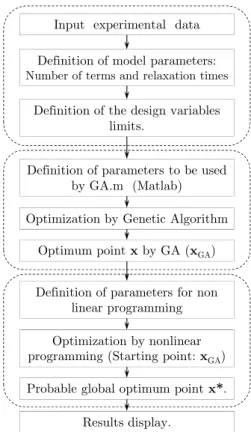
3.3 Computational Implementation
Initial results of the identification process based only on non-linear programming techniques (NLP) indicated the existence of several local minima points. Thus, obtaining the optimal properties strongly depends on the initially arbitrated point in the optimization process. In order to avoid such problem, the identification methodology proposed in the present work is anchored on a hybrid op-timization technique. Such computational process, showed in Fig. 2, was implemented in a set of routines in the MatLab® software. First of all, the experimental data are read, followed by the defi-nition of the parameters for executing the routine through genetic algorithms (GA), and the respec-tive optimization process. Subsequently, the best point obtained from the optimization process by GA is used as entry datum for the NLP routine and its execution. As the optimization technique by GA is not deterministic, and having in mind the aim of increasing the probability of finding the global optimum point, the hybrid optimization process (GA and NLP) is performed 10 times, which is an arbitrated number. The optima material parameters are taken considering the set of values that produces the smallest quadratic relative distance D2
. In this optimization process, functions ga.m and fmincon.m (belonging to the MatLab® toolbox) were used.
The parameters used in the optimization process by GA are: population size is 100; number of generations is 1000; stop tolerance is 1.0E-8 (the algorithm stops when the average relative shift along generations is smaller or equal to the set value); and mutation rate is 0.02. The optimization process by NLP is based on the quadratic sequential programming method where the Hessian ma-trix of the objective function is updated through the Broyden-Fletcher-Goldfarb-Shanno (BFGS) method. The optimization parameters by NLP are: maximal number of evaluations of the function is 1000, maximal number of iterations allowed is 600, and stop tolerance is 1.0 e-10.
The upper and lower limits of the material parameters were defined by: 0.02 £ n £ 0.98, 0 MPa £E¥ £ 10 MPa, 1.001 £rm £ 3000.0, 1.0 e-8 s £ ta £ 5.0 s, 0.00 £C1 £ 200.0 and 0.0
o
C £C2 £ 8000.0o C. It is important to point out that the choice of those limiting values was
per-formed through numerical experiments, but taking care so as not to allow the optimum point to lie in the frontier of the design space, except for the performance of tests at a single temperature.
3.4 Validation of the Proposed Approach
Input experimental data
Definition of model parameters: Number of terms and relaxation times
Definition of the design variables limits.
Definition of parameters to be used by GA.m (Matlab)
Optimization by Genetic Algorithm
Optimum point xby GA (xGA)
Definition of parameters for non linear programming
Optimization by nonlinear programming (Starting point: xGA)
Probable global optimum point x*.
Results display.
Figure 2: Flowchart of the computational structure implemented in the
MatLab® software for characterizing VEM.
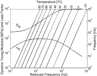
From the nomogram provided by the manufacturer (Fig. 3) several curves are constructed, with constant temperatures for each curve. Having those curves, an adjustment is made by the ordinary least squares method in order to obtain the material parameters in frequency domain. In this case, considering the constitutive model of fractional Zener, the expression for the complex Young modu-lus presented by Pritz (2003) is
(
)
(
)
(
)
( )
( )
T
T R
R R G R
R
E E i
E , T E . i
i
b
b f
h f
¥
+ W é ù
W = = W ë + W û
+ W
0 0
0
1
1 (43)
where WR is the reduced frequency (given by W = WR aT
( )
T , where W is the circular frequency in rad/s), ER( )
WR is the dynamic Young modulus, and hG( )
WR is the loss factor of VEM. These functions are graphically represented in Fig. 3. This way, the material parameters corresponding to the master curve shown in Fig. 3 are identified, including the WLF model parameters. The results obtained in such identification are: E0 = 6.989 MPa, E¥ = 9863 MPa, f0 =1.59 e-3 sbT,
T
Figure 3: Reduced frequency nomogram for EAR C-2003.
Thus, when the material parameters of VEM in frequency domain are known, it is possible to perform an interconversion to time domain and obtain the properties of the model in that space. Therefore, the Fourier Transform is applied to each term of the differential equation of the FZ mod-el (Eq. 16) and, considering the influence of temperature, the constitutive equation of the described model in frequency domain, WR, is given by
(
)
( )
(
) ( )
a i R R E r a i R R
n n
n n
m
t s ¥ t e
é + W ù W = é + W ù W
ê ú ê ú
ë1 û ë1 û (44)
In this case, s
( )
WR and e( )
WR are the normal stress and longitudinal strain in the material, respectively, both described in frequency domain.Defining the complex Young modulus as E
( )
WR = s( ) ( )
WR e WR , in Eq. 44, one has(
)
(
)
(
)
a R
a R
E E r i
E ,T
i
n n m
n n
t t
¥ + ¥ W
W =
+ W
1 (45)
Comparing Eqs. 43 and 45, one obtains the following correspondences of material parameters
between time and frequency domains: n = bT, E¥ = E0, rm = E¥ E0 and T
a b
t = f
1
0 . The
values of the material parameters in time domain of the reference material (EAR C–2003) are pre-sented in the last column of Tab. 1.
From the material parameters in time domain, six ‘pseudo-experimental tests’ were generated at temperatures T1 = -20
o C,
T2 = +20 o C,
T3 = +41,9
o C and
T4 = +60
o C and at strain rates
A
e = 0.0001, eB = 0.003 and eC = 0.100 (mm/mm)/s. For each pseudo-experimental test, stresses were obtained via constitutive relationship based on the FZ model (Eq. 26).
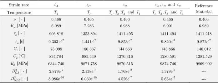
temperatures, T1, T2, T3, and T4; and all rates and temperatures simultaneously. The results
ob-tained in such process are presented in Tab. 1. In that table, besides the 6 material parameters rep-resenting the design variables vector, other parameters are included: E0, which is the instantaneous
relaxation modulus (Eq. 18); DGA2
, which is the optimal average quadratic distance obtained in the GA; and DNLP2
, which is the same variable obtained when the technique is the NLP.
Strain rate eA eC eB eA,eB and eC Reference
Material
Temperature T4 T1 T1,T2,T3 and T4 T1,T2,T3 and T4
n [ - ] 0.466 0.465 0.466 0.466 0.466
E¥[MPa] 6.989 7.286 6.988 6.991 6.989
rm[ - ] 906.818 1353.894 1411.495 1411.494 1411.218
a
t [s] 9.303 e-7 1.441e-7 9.853e-7 9.820e-7 9.872e-7
C1[ - ] 75.098 180.337 144.663 145.866 146.012
C2[
oC] 834.784 985.449 1270.316 1280.591 1281.529
0
E [MPa] 6344.740 9871.758 9870.515 9874.746 9869.992
G A D2
[ - ] 2.878e-7 2.138e-7 1.768e-2 1.378e-5 ---
NLP
D2 [ - ]
8.086e-10 6.030e-10 4.526e-7 5.664e-7 ---
Table 1: Solutions found in the identification process using the EAR C–2003 material.
Observing Tab. 1, one notices that the identification using all combinations of temperatures and rates presents better convergence of the parameters when compared to the reference material. As expected, the test performed at a fast strain rate (eC =0.100 (mm/mm)/s) and cold temperature
( )
T1 , provides a more precise estimate of the relaxation instantaneous modulusE0. On the otherhand, using a very low strain rate (eA =0.0001 (mm/mm)/s) and high temperature
( )
T4 , we notethe better convergence to the equilibrium relaxation modulus, E¥. Also, it can be highlighted the
convergence of the results obtained in the numerical test with all temperatures, simultaneously, and a unique intermediary rate strain (eB =0.0030 (mm/mm)/s). Thus, the results show that the pro-posed methodology converges, and that the best results are obtained when several curves are evalu-ated simultaneously.
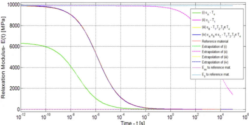
Entering the values presented in Tab. 1 in Eq. 17, one obtains the relaxation modulus function, viewed in Fig. 4. This function considers the history of all temperatures and strain rates, and repre-sents the master curve for a reference temperature (in this case, 41.9 oC) obtained through the op-timization process. It is possible to observe that the best result obtained presents very low level of error when compared to the reference material curve, for the curves almost overlap.
Figure 4: Relaxation modulus of the EAR C-2003 material considering the cases in Tab 1.
4 RESULTS AND DISCUSSIONS
This section presents the results obtained in the process of identifying the CYCOLAC BDT5510 material. This material is a polymer of the Acrylonitrile Butadiene Styrene type (ABS) manufac-tured by SABIC®. The experiments were performed according to the ASTM D638 norm, consider-ing four different temperatures (T1 = -40
o C, T = +
2 23
o C, T = +
3 43
o C, and T = +
4 66
o C)
and, at each temperature, the material was subjected to traction uniaxial with a fixed strain rate equal to 0.0833 (mm/mm)/s.
The difference between this section and the previous one is that, here, the experimental data do not result from ‘pseudo-tests’. Fig. 5 presents the experimental data (+) and the corresponding stress-strain deformation curves considering the FZ constitutive model (Eq. 27), obtained from the identification process, for a strain rate of 0.0833 (mm/mm)/s.
Tab. 2 presents the results obtained in the identification process, considering the analysis of each temperature individually under a single strain rate, as well as the simultaneous analysis of all temperatures involved. In all analyses, the reference temperature is 23 oC.
Figure 5: Stress-strain curves considering the FZ constitutive model (-) with experimental
Temperature T1 T2 T3 T4 T1,T2,T3, and T4
n [ - ] 0.088 0.189 0.98 0.98 0.256
E¥[MPa] 5.885 1.104 0.094 0.086 0.613
rm[ - ] 122.339 1131.749 2482.617 2508.986 545.069
a
t [s] 2.417e-4 3.827e-5 4.322 1.657 1.646
C1[ - ] 0.00 --- 198.462 96.062 174.008
C2[
oC]
1302.866 --- 4109.632 7055.094 7074.586
0
E [MPa] 725.800 1251.024 233.409 214.498 334.798
GA
D2 [ - ]
9.029e-5 2.003e-3 3.066e-4 2.586e-4 3.283e-3
NLP D2
[ - ] 6.066e-5 1.576e-3 2.985e-4 2.583e-4 3.282e-3
Table 2: Numerical results arising from the identification process considering
the influence of temperature of the CYCOLAC BDT5510 material.
The results obtained considering all the curves, simultaneously, are presented in the Fig. 6. It is observed that the results of the characterization process of the polymer under study fit to the exper-imental curves, with low values on the quadratic difference, ( 2
PNL
D ), between the numerical and
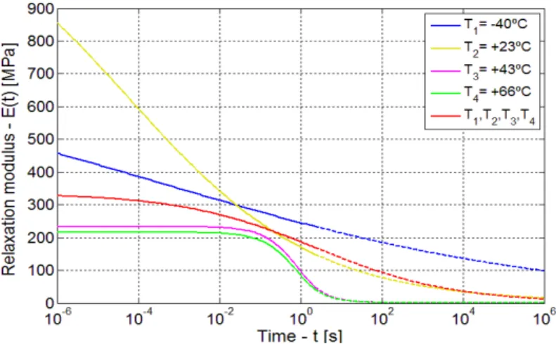
experimental functions. The numerical values are shown in Tab. 2. Fig. 7 shows the graphical repre-sentation of the relaxation modulus functions of the results presented in Tab. 2.
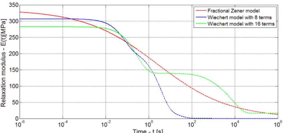
The results obtained previously are confronted with results obtained by a similar identification process, but using another constitutive model. In that case, the methodology used is presented by Pacheco et al. (2015) and refers to VEMs characterization, in time domain, but using the Prony series, via Weichert’s constitutive model, which are based on constitutive equations of integer order. In the present model, the relaxation modulus is given by
(
)
T it NT
i i
E t,T E E e a t
-=
= 0 +
å
1
(46)
where Ei -ti (i =1, …, NT) represents the stiffness-relaxation time pair of each Maxwell element in the constitute Weichert’s model. The characterization was performed considering the fixed relax-ation times ti where t1 =1.0 e
-2 s and
NT
t =1.0 e4 s. In this case, NT is the number of terms used in the series. The intermediate relaxation times were arbitrated through a homogeneous spac-ing in a logarithmic scale of time.
a) T1 = –40o C b) T2 = 23o C
c) T3 =43o C d) T
4 = 66o C
Figure 6: Simultaneous adjust of the curves using the theoretical model of FZ (-) with the experimental
data (+) of CYCOLAC BDT5510 material, considering the influence of temperature by WLF.
Figure 7: Identified relaxation modulus functions considering a strain rate of 0.0833 ((mm/mm)/s)
Figure 8: Comparison between the relaxation modulus functions obtained via FZ model and Weichert's model – CYCOLAC BDT5510 material.
5. CONCLUSIONS
The present work proposes a methodology for characterizing VEM in time domain, on the basis of the Fractional Zener constitutive model under the influence of temperature, here considered via WLF model. The methodology developed allows characterizing viscoelastic materials with a simple thermorheologically behavior. To this end, experimental data extracted from stress-strain curves at different strain rates and temperatures were used as a starting point. Having these curves in mind, a reverse identification problem was proposed aiming at reducing the quadratic distance between the experimental stress-strain curves and the corresponding ones given by the theoretical model. The formulation was implemented in the Matlab® software and a hybrid optimization technique (GA and NLP) was used.
The evaluation of the model using a real VEM (EAR C–2003), but with experimental pseudo-tests, under the results obtained via simultaneous rates and temperatures, presents a good level of convergence. This becomes evident in the graphical representation of the relaxation modulus func-tions, when a superposition of curves occurs from the results obtained via the proposed methodology and from the results obtained by the interconversion between frequency and time domains. Fur-thermore, it was observed that the test performed at a low strain rate and high temperature pro-vides a good convergence for the equilibrium relaxation modulus, E∞. Moreover, tests with high strain rate and low temperatures result in good estimates of instantaneous relaxation modulus, E0.
Although this approach enables the identification of the relaxation module with few pure tensile tests, it is clear that these tests must be conducted in a suitable and wide range of temperatures and strain rates which enable the acquisition of information for better curve fit throughout your domain. The results indicate that the methodology is adequate for characterizing VEMs in time domain, provided they are thermorheologically simple materials.
Acknowledgements
References
Bagley, R. L., Torvik, P. J. (1985). Fractional calculus in the transient analysis of viscoelastically damped structures. AIAA Journal, 23(6): 918-925.
Brinson, H. L., Brinson, L. C. (2008). Polymer Engineering Science and Viscoelasticity, Springer Verlag (New York). Chae, S. H., Zhao, J. H., Edwards, D. R., Ho P. S. (2010). Characterization of the viscoelasticity of molding com-pounds in the time domain. Journal of Electronic Materials, 39(4): 419-425.
Christensen, R. M. (1982). Theory of Viscoelasticity: An Introduction. 2nd ed., Academic Press (New York). Gorenflo, R., Loutchko, J., Luchko, Y. (2002). Computation of the Mittag-Leffler function E̝̞(z) and its deriva-tive. Fractional Calculus & Applied Analysis, 5(4): 491-518.
Gorenflo, R., Loutchko, J., Luchko, Y. (2003). Correction: “Computation of the Mittag-Leffler function E̝, ̞ (z) and its derivative” [Fractional Calculus & Applied Analysis, (2002), 5(4): 491–518]. Fractional Calculus & Applied Anal-ysis, 6(1): 111-112.
Haubold, H. J., Mathai, A. M., Saxena, R. K. (2011). Mittag-Leffler functions and their applications. Journal of Applied Mathematics, 2011: 1-51.
Jiménez, A. H., Santiago, J. H., Garcia, A. M., González, J. S. (2002). Relaxation modulus in PMMA and PTFE fitting by fractional Maxwell model. Polymer Testing, 21(3): 325-331.
Kilbas, A. A., Srivastava, H. M., Trujillo, J. J. (2006). Theory and Applications of Fractional Differential Equations. Elsevier (Amsterdan).
Lakes, R. S. (2004). Viscoelastic measurement techniques. Review of Scientific Instruments, 75(4): 797-810.
Lakes, R., Capodagli, J. (2008). Isothermal viscoelastic properties of PMMA and LDPE over 11 decades of frequency and time: a test of time-temperature superposition. Rheologica Acta, 47(7): 777-786.
Li, C., Zeng, F. (2015). Numerical Methods for Fractional Calculus. CRC Press (Florida).
Liu Q., Subhash, G. (2006). Characterization of viscoelastic properties of polymer bar using iterative deconvolution in the time domain. Mechanics of Materials, 38(12): 1105-1117.
Mainardi, F. (2010). Fractional Calculus and Waves in Linear Viscoelasticity: An Introduction to Mathematical Models. Imperial College Press (London).
Mainardi, F., Spada, G. (2011). Creep, relaxation and viscosity properties for basic fractional models in rheology. European Journal of Physics Special Topics, 193(1): 133-160.
Martinez-Agirre, M., Elejabarrieta, M. J. (2010). Characterization and modeling of viscoelastically damped sandwich structures. International Journal of Mechanical Sciences, 52(9): 1225-1233.
Moreira, R. A. S., Melo, F. J. Q., Rodrigues, J. F. D. (2010). Static and dynamic characterization of composition cork for sandwich beam cores. Journal of Materials Science, 45(12): 3350-3366.
Moschen, I. D. C. (2006). Sobre as Funções Mittag-Leffler e o Modelo Fracionário de Materiais Viscoelástico. Ph.D. Dissertation, Universidade Federal de Santa Catarina (in Portuguese).
Pacheco, J. E. L., Pereira, J. T., Bavastri, C. A. (2015). Viscoelastic relaxation modulus characterization using Prony series. Latin American Journal of Solids and Structures, 12(2): 420-445.
Park, S. W. (2001). Rheological modeling of viscoelastic passive dampers. Proceedings of SPIE 4331, Smart Struc-tures and Materials 2001: Damping and Isolation, 343.
Plaseied, A., Fatemi, A. (2008). Deformation response and constitutive modeling of vinyl ester polymer including strain rate and temperature effects. Journal of Materials Science, 43(4): 1191-1199.
Pritz, T. (1996). Analysis of four-parameter fractional derivative model of real solid materials. Journal of Sound and Vibraton, 195(1): 103-115.
Rektorys, K. (1980). Variational Methods in Mathematics. Science and Engineering. D. Reidel Publishing Company (Boston).
Shukla, A. K., Prajapati, J. C. (2007). On a generalization of Mittag-Leffler function and its properties. Journal of Mathematical Analysis and Applications, 336(2): 797-811.
Tschoegl, N. W., Knauss, W. G., Emri, I. (2002). The effect of temperature and pressure on the mechanical proper-ties of thermo- and/or piezorheologically simple polymeric materials in thermodynamic equilibrium – A critical re-view. Mechanics of Time-Dependent Materials, 6(1): 53-99.
Welch, S. W. J., Rorrer, R. A. L., Duren Jr., R. G. (1999). Application of time-based fractional calculus methods to viscoelastic creep and stress relaxation of materials. Mechanics of Time-Dependent Materials, 3(3): 279-303.