www.atmos-meas-tech.net/3/187/2010/
© Author(s) 2010. This work is distributed under the Creative Commons Attribution 3.0 License.
Measurement
Techniques
Aerodynamic gradient measurements of the NH
3
-HNO
3
-NH
4
NO
3
triad using a wet chemical instrument: an analysis of precision
requirements and flux errors
V. Wolff1,*, I. Trebs1, C. Ammann2, and F. X. Meixner1,3
1Max Planck Institute for Chemistry, Biogeochemistry Department, P.O. Box 3060, 55020 Mainz, Germany 2Agroscope ART, Air Pollution and Climate Group, 8046 Z¨urich, Switzerland
3Department of Physics, University of Zimbabwe, P.O. Box MP 167, Harare, Zimbabwe *now at: Agroscope ART, Air Pollution and Climate Group, 8046 Z¨urich, Switzerland Received: 15 July 2009 – Published in Atmos. Meas. Tech. Discuss.: 8 October 2009 Revised: 14 January 2010 – Accepted: 19 January 2010 – Published: 10 February 2010
Abstract. The aerodynamic gradient method is widely used for flux measurements of ammonia, nitric acid, par-ticulate ammonium nitrate (the NH3-HNO3-NH4NO3triad) and other water-soluble reactive trace compounds. The sur-face exchange flux is derived from a measured concentration difference and micrometeorological quantities (turbulent ex-change coefficient). The significance of the measured con-centration difference is crucial for the significant determina-tion of surface exchange fluxes. Addidetermina-tionally, measurements of surface exchange fluxes of ammonia, nitric acid and am-monium nitrate are often strongly affected by phase changes between gaseous and particulate compounds of the triad, which make measurements of the four individual species (NH3, HNO3, NH+4, NO−3) necessary for a correct interpre-tation of the measured concentration differences.
We present here a rigorous analysis of results obtained with a multi-component, wet-chemical instrument, able to si-multaneously measure gradients of both gaseous and particu-late trace substances. Basis for our analysis are two field ex-periments, conducted above contrasting ecosystems (grass-land, forest). Precision requirements of the instrument as well as errors of concentration differences and micromete-orological exchange parameters have been estimated, which, in turn, allows the establishment of thorough error estimates of the derived fluxes of NH3, HNO3, NH+4, and NO−3. De-rived median flux errors for the grassland and forest field experiments were: 39% and 50% (NH3), 31% and 38% (HNO3), 62% and 57% (NH+4), and 47% and 68% (NO−3), respectively. Additionally, we provide the basis for using
Correspondence to:V. Wolff ([email protected])
field data to characterize the instrument performance, as well as subsequent quantification of surface exchange fluxes and underlying mechanistic processes under realistic ambi-ent measuremambi-ent conditions.
1 Introduction
188 V. Wolff et al.: An analysis of precision requirements and flux errors increased particle formation (Erisman and Schaap, 2004). In
order to address these problems, so-called critical loads have been introduced, as quantitative estimates of the deposition of one or more pollutants below which significant harmful effects on specified elements of the environment do not oc-cur according to the present knowledge (Cape et al., 2009; Plassmann et al., 2009). Hence, the knowledge of exchange processes and deposition rates of these compounds is funda-mental for atmospheric research and for policy makers.
NH3 and HNO3 are polar molecules, which are highly water-soluble and exhibit a high affinity towards surfaces. Therefore, the measurement of these compounds with high temporal resolution is a challenge under atmospheric condi-tions. Particulate compounds usually feature low deposition velocities, hence they typically exhibit very small concentra-tion gradients in the surface layer, demanding high precision instruments to measure vertical concentration differences of these species (e.g., Erisman et al., 1997). To characterize the surface exchange of the NH3-HNO3-NH4NO3 triad, simul-taneous measurements of NH3, HNO3, particulate NH+4 and NO−3 are mandatory and they should be highly selective with respect to gaseous and particulate phases.
Direct measurements of surface-atmosphere exchange fluxes may be provided by the eddy covariance method, but it requires fast response trace gas sensors. Some newly devel-oped fast instruments have been tested and validated recently (e.g., Brodeur et al., 2009; Farmer et al., 2006; Huey, 2007; Nemitz et al., 2008; Schmidt and Klemm, 2008; Zheng et al., 2008). Their major drawback is the restricted applica-bility to a single compound, not allowing for the character-ization of the entire NH3-HNO3-NH4NO3triad. Moreover these instruments are still under development, and their de-tection limit is still too high to measure in remote environ-ments (Nemitz et al., 2000).
Thus, to date, the aerodynamic gradient method (AGM) is still the commonly applied technique to measure NH3, HNO3and NH4NO3surface exchange fluxes (e.g., Businger, 1986; Erisman and Wyers, 1993; Nemitz et al., 2004a; Phillips et al., 2004). Surface-atmosphere exchange fluxes are derived from measurements of vertical concentration dif-ferences by instruments with much lower time resolution than covariance techniques. The AGM requires average concentrations (over 30–60 min) measured at two or more heights above the investigated surface or vegetation canopy.
Most studies that investigated the surface-atmosphere ex-change fluxes of NH3, HNO3and particulate NH+4 and NO−3 did not consider errors of the applied measurement tech-niques, nor did they present errors of the calculated fluxes and deposition velocities (Businger and Delany, 1990). How-ever, error estimates and/or confidence intervals of the results are an important part of a thorough analysis and presentation of any measurement results and their scientific interpretation (Miller and Miller, 1988).
In this study, we evaluate the performance of the novel GRAEGOR instrument (GRadient of AErosol and Gases On-line Registrator; ECN, Petten, NL) recently described by Thomas et al. (2009) for aerodynamic gradient measure-ments of NH3, HNO3, NH+4, and NO−3 to determine ex-change fluxes under representative environmental conditions. GRAEGOR is a wet chemical instrument for the quasi-continuous measurement of two-point vertical concentration differences of water-soluble reactive trace gas species and their related particulate compounds. We use results from two field campaigns to investigate (a) the precision requirements of the concentration measurements above different ecosys-tems under varying micrometeorological conditions, (b) the error of the concentration difference measured with GRAE-GOR, (c) the error of the micrometeorological exchange pa-rameter (the transfer velocity,vtr), and (d) the resulting flux error. The experiments were conducted over contrasting ecosystems, a grassland site with low canopy height, low aerodynamic roughness and high nutrient input, and a spruce forest site with tall vegetation, high aerodynamic roughness and low nutrient state. Due to the differences in micrometeo-rological as well as in nutrient balance conditions, exchange processes are expected to be different.
For the first time, a wet-chemical multi-component instru-ment is characterized in terms of the instruinstru-ment precision to resolve vertical concentration differences and the associated errors of surface-atmosphere exchange fluxes.
2 Experimental
2.1 Site descriptions
2.1.1 Grassland site, Switzerland (NitroEurope)
relative humidities below 30%. This warm period was fol-lowed by some episodes of rain and cloud cover leading to lower temperatures (<10◦C). The grassland consists of grass
species as well as legumes and some herb species (Ammann et al., 2007), its canopy height grew during our study from around 0.08 to 0.25 m.
2.1.2 Spruce forest site, Germany (EGER)
The second experiment was conducted within the framework of the project EGER (ExchanGe processes in mountainous Regions) at the research site “Weidenbrunnen” (50◦08′N, 11◦52′E; 774 m a.s.l.), a Norway spruce forest site located in a mountainous region in south east Germany (Fichtelgebirge) in summer/autumn 2007 (25 August – 3 October). The sur-rounding mountainous area extends approx. 1000 km2 and is covered mainly with forest, agricultural land including meadows and lakes. It is located in the transition zone from maritime to continental climates with annual average tem-peratures of 5.0◦C (1971–2000; Foken, 2003) and average annual precipitation sum of 1162 mm (1971–2000; Foken, 2003). The study site has been maintained for more than 10 years by the University of Bayreuth and a variety of stud-ies have been conducted there (Falge et al., 2005; Held and Klemm, 2006; Klemm et al., 2006; Rebmann et al., 2005; Thomas and Foken, 2007; Wichura et al., 2004). The stand age of the Norway spruce (Picea abies) was approx. 54 years (according to Alsheimer, 1997), the mean canopy height was estimated to be 23 m (Staudt, 2007), and the single sided leaf area index was 5.3. Measurements were performed on a 31 m walk-up tower. During the EGER measurements in 2007, temperatures were generally quite low (around 10◦C) and
the relative humidity often remained above 80% throughout the day. Only few days with higher temperatures of up to 22◦C and lower relative humidity (50–60%) were encoun-tered.
2.2 Measurement method
2.2.1 GRAEGOR
The GRAEGOR (Thomas et al., 2009) is a wet chemi-cal instrument for semi-continuous, simultaneous two-point concentration measurements of water-soluble reactive trace gases (NH3, HNO3, HONO, HCl, and SO2)and their related particulate compounds (NH+4, NO−3, Cl−, SO2−
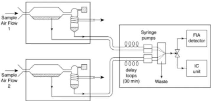
4 ). GRAE-GOR collects the gas and particulate samples simultaneously at two heights using horizontally aligned wet-annular rotat-ing denuders and steam-jet aerosol collectors (SJAC), respec-tively (see to Fig. 1). The combination of the denuder and the SJAC sampling devices is similar to the MARGA system (instrument for Measuring AeRosol and GAses, ten Brink et al., 2007). Air is simultaneously drawn through the sam-ple boxes, passing first the wet-annular rotating denuders, where water-soluble gases diffuse from a laminar air stream
Fig. 1.Simplified scheme of the GRAEGOR instrument.
into the sample liquid. In both SJACs, the sample air is then mixed with water vapour from double-de-ionized wa-ter and the supersaturation causes particles to grow rapidly (within 0.1 s) into droplets of at least 2 µm diameter. These droplets, containing the dissolved particulate species are then collected in a cyclone (cf. Trebs et al., 2004). The airflow through the two sample boxes is∼14 L min−1(at STP=0◦C and 1013.25 hPa) per box and is kept constant by a critical orifice downstream of the SJAC. Liquid samples are sequen-tially analyzed online using ion chromatography (IC) for an-ions and flow injection analysis (FIA) for NH3and particulate NH+4. Within each full hour GRAEGOR provides one half-hourly integrated gas and particulate concentration for each height for each species (one sequential analytical cycle of all four liquid samples (two denuder, two SJAC samples) takes one hour, cf. Thomas et al., 2009).
Syringe pumps in the analytical box (Fig. 1) provide sta-ble liquid flows, which has improved the accuracy of the instrument in comparison to previous studies (cf. Trebs et al., 2004). Prior to analysis an internal bromide standard is added to each sample. Additionally to its use in the de-termination of the concentration value, it is used in com-bination with monitoring the FIA waste flow as an internal quality indicator, enabling the identification of poor chro-matograms (high/noisy baseline, bad peak shapes), high double-de-ionized water conductivity and unstable flows.
190 V. Wolff et al.: An analysis of precision requirements and flux errors 2.2.2 Calibration and errors of the concentration
measurements
The FIA cell was calibrated using liquid standards once a week, while the IC response was checked with liquid stan-dards once or twice during each experiment. Field blanks representing the zero concentration signal of the system were measured once a week by switching off the sampling pumps and sealing the inlets, leaving the rest of the system un-changed (see Thomas et al., 2009). The random error of the measured air concentrations of NH3, HNO3, NH+4 and NO−3 was calculated according to Trebs et al. (2004) and Thomas et al. (2009) using Gaussian error propagation. The concentration error depends on the individual random errors of the sample airflow, the liquid sample flow, the bromide standard concentration and the peak integration. Follow-ing suggestions by Thomas et al. (2009), the field perfor-mance of GRAEGOR was checked not only by monitoring the FIA waste flow, double-de-ionized water conductivity, and IC performance, but also by (a) measuring the air flow through the sample boxes with an independent device (Gili-brator, Gilian, Sensodyne) once per day and (b) measuring and adjusting the liquid flow supply of the SJAC once per week. Additionally, other factors may affect the sample ef-ficiency of the sample boxes. Therefore, the coating of the denuders was visually checked at least once per day and also the inlets were checked every day for visible contamination and water droplets.
2.2.3 Determination of the concentration difference error
Evaluating potential error sources of the concentrations mea-sured by GRAEGOR, it is obvious that some of them (e.g., the error of the bromide standard, see Sect. 2.2.2) do not influence the error of the difference between the concen-trations,σ1C, sampled by the two individual sampling boxes because the same analytical unit and the same standard solu-tions are used for deriving both concentrasolu-tions. Some of the error sources of an individual concentration value are, how-ever, relevant for1C, as they may theoretically impact the concentrations at the two heights differently (e.g., the airflow through the sample boxes and the liquid flows). Additionally, other factors may introduce different sample efficiency of the sample boxes and thus impact on the precision of1C. Thus, the determination ofσ1Cis not to be performed straight for-ward from the error in concentrations.
Some of the factors lead to random errors, i.e., to a scat-ter in both directions around a “true value”, whereas some of them may lead to temporal or non-temporal systematic errors, such as constant different sampling efficiencies. In order to investigate and characterize these errors, we per-formed extended side-by-side measurements during our field experiments, as integrated error analysis for1C. The sam-ple boxes were regularly placed side-by-side during time
periods of different length, but totally of 352 h (NEU) and of 255 h (EGER). During NEU, sampling could be performed through one common inlet at z=0.9 m above ground, since the boxes were located close to the ground. During EGER, the two boxes were standing next to each other (24.4 m above ground), with a distance of 0.4 m between the inlets. Dur-ing NEU, four side-by-side measurement periods were per-formed, while during EGER, due the difficult set up at the tower, we confined ourselves to two side-by-side measure-ment periods at the beginning and the end of the experimeasure-ment. We plotted the concentrations measured with the two sam-ple boxes side-by-side against each other and made an or-thogonal fit through the scatter plots by minimizing the per-pendicular distances from the data to the fitted line. That way, both concentration values are treated the same way, tak-ing into account that both concentrations may be prone to measurement errors. We define a consistent deviation from the 1:1 line as systematic difference between the concentra-tion measurements and we correct for it applying the calcu-lated fit-equation. We regard the remaining scatter around the fit as random error between the concentration measurements of the two boxes.
2.3 The aerodynamic gradient method (AGM)
Applying the AGM the turbulent vertical transport of an en-tity towards to or away from the surface is, in analogy to Fick’s first law, considered as the product of the turbulent dif-fusion (transfer) coefficient and the vertical air concentration gradient∂C/∂zin the so-called constant flux layer (Foken, 2006).
FC= −KH(u∗,z,L)·
∂C
∂z (1)
Usually, the turbulent diffusion coefficients for scalars (sen-sible heat, water vapour, trace compounds) are assumed to be equal (Foken, 2006). The turbulent diffusion coefficient for sensible heat,KH, expresses both, the mechanic turbulence, induced by friction shear (expressed through the friction ve-locity,u∗)and the thermal turbulence induced by the ther-mal stability of the atmosphere (expressed inz/L). It is thus a function of the heightz(m) above the zero plane displace-ment heightd (m), and atmospheric stability, parameterized by the Obukhov lengthL(m):
L= − u
3 ∗
κ·Tg·ρH
·cp
(2)
whereu∗ is the friction velocity (m s−1), g the acceleration of gravity (m s−2),T the (absolute) air temperature (K),H
the turbulent sensible heat flux (W m−2), ρ the air density (kg m−3),cpthe specific heat of air at constant pressure, and
κ the von Karman constant (0.4) (Arya, 2001). H andu∗
For practical reasons, the flux-gradient relationship is usu-ally not applied in the differential form (Eq. 1) but in an in-tegral form between two measurement heights,z1andz2(in m); accordingly the flux is derived from the difference in con-centration,1C=C2−C1(in µg m−3), measured at the two heights, as (Mueller et al., 1993):
FC= −
u∗·κ
lnz2
z1
−9H zL2
+9H zL1
| {z }
=vtr
·1C (3)
withκthe von Karman constant (0.4) and9H, the integrated stability correction function for sensible heat (equal to that of trace compounds). The left term of the product on the right hand side of Eq. (3) is often referred to as the trans-fer velocity,vtr (m s−1). It represents the inverse resistance of the turbulent transport between the two heightsz1andz2 (Ammann, 1998). Note here, that we use all measurement heightsz1,z2, andz, as aerodynamic heights above the zero plane displacement height,d. For the grassland site (NEU) with varying canopy heighthcanopy,d (in m above ground) was estimated asd=0.66·(hcanopy−0.06)according to Nef-tel et al. (2007), and for the forest site (with constant canopy height during our study) it was determined as 14 m above ground (Thomas and Foken, 2007).
When applying the AGM the accurate measurement of the concentration difference of the substance of interest is the major challenge. This is especially the case in remote en-vironments, where concentrations are very low (Wesely and Hicks, 2000) and vertical concentration differences are in the order of 1 to 20% of the mean concentration (Businger, 1986; Foken, 2006).
Above high canopies, such as forests, the profiles of mete-orological parameters have been found to deviate from their ideal shape within the so-called roughness sublayer (Foken, 2006). In this layer the use of flux gradient relations may underestimate scalar fluxes by 10% or more (Cellier and Brunet, 1992; Garratt, 1978; H¨ogstr¨om, 1990; Simpson et al., 1998; Thom et al., 1975). The deviations from the ideal shape are site specific as well as scalar specific. Unfortu-nately we do not dispose of reliable site and scalar specific parameters within the present experiment. Therefore we ap-plied the conservative calculation approach not including a correction factor for scalars. It has to be noted that the use of directly measuredu∗ (with eddy covariance) already ac-counts for the enhancement of momentum flux in compari-son to the original AGM method based on wind speed pro-files (Garratt, 1992).
2.4 Flux error analysis
When applying the AGM for measurements of two point ver-tical concentration differences, the flux is determined from the product of1Candvtr.(see Eq. 3). A flux error thus in-cludes the errors of factors,σ1C andσvtr. σ1C is derived
from side-by-side measurements as described in Sect. 2.2.3.
σvtr will be estimated from errors of the main influencing
pa-rameters ofvtras described in Sect. 4.4.
These two errors,σ1C andσvtr, have different effects on
the resulting flux, its sign, magnitude and error. The sign of
1Cdetermines the sign and therefore the direction of the de-rived flux. Thus,σ1Cis a measure of the significance of the derived flux direction, additionally to the influence ofσ1C on the magnitude of the flux error. The error of vtr how-ever, expresses the uncertainty in the velocity of exchange and therefore influences the magnitude of the flux error, but
σvtr does not impact the significance of the flux sign. From
σ1Cwe can deduce the significance of a difference from zero and subsequently of the flux direction. The error of the flux,
σF, we deduce by combining the two values,σ1C andσvtr,
using Gaussian error propagation:
σF=F· s
σvtr
vtr 2 + σ1C 1C 2 (4)
3 Constraints for the precision – theoretical approach
To obtain an estimate of the precision required to resolve ver-tical concentration gradients with regard to stability and mea-surement heights using Eq. (3), an independent flux estimate is necessary. For components that typically feature unidirec-tional deposition fluxes, such as HNO3, the so-called infer-ential method may be used to obtain a maximum deposition flux estimate. The inferential method is based on the “big leaf multiple resistance approach” (Hicks et al., 1987; We-sely and Hicks, 2000). In analogy to Ohm’s law, the flux of HNO3is expressed as the ratio of the HNO3concentration,
CHNO3 at one height and the resistances against deposition to the ground. This resistance consists of three individual re-sistancesRa,Rb, andRc, each of them characterizing part of the deposition process:
FHNO3= −
1
Ra+Rb+Rc·
CHNO3 (5)
with FHNO3 denoting the HNO3 deposition flux
(µg m−2s−1), R
a the aerodynamic resistance (s m−1),
Rb the quasi-laminar or viscous boundary layer resistance (s m−1), Rc the surface resistance (s m−1)and CHNO3 the concentration of HNO3(µg m−3).Rais calculated according to Garland (1977). It is defined for a measurement heightz
(m) above a surface of roughness lengthz0(m):
Ra(z,z0)= 1
κ·u∗
ln z z0 −9H
z
L
(6) The roughness length,z0, of the grassland site was derived from wind and turbulence measurements (Neftel et al., 2007) as a function of the canopy height: z0=0.25· hcanopy−d
192 V. Wolff et al.: An analysis of precision requirements and flux errors
z0of 2 m (Thomas and Foken, 2007).Rbdetermines the ex-change immediately above the vegetation elements and can be described by (Hicks et al., 1987):
Rb= 2
κ·u∗
Sc P r 2 3 (7) whereScandP r are the Schmidt and Prandtl number, re-spectively. P r is ≈0.72 and Sc is a strong function of the molecular diffusivity of the trace gas (for HNO3≈1.25) (Hicks et al., 1987). Due to the high surface affinity and the observed high deposition rates of HNO3, the canopy re-sistance,Rc, is often assumed to be zero (e.g., Hanson and Lindberg, 1991; Sievering et al., 2001) and thus, the theoret-ical maximum deposition flux of HNO3towards the surface can be obtained by:
FmaxHNO3= − 1
Ra+Rb·
CHNO3 (8)
This maximum HNO3 flux value (calculated with C2 at heightz2)will be used to estimate the minimal requirements which the instrument’s precision must satisfy to determine fluxes with the AGM at the two sites for a range of atmo-spheric stabilities.
3.1 Influence of atmospheric stability
Combining Eqs. (3) and (8) we may calculate a maximum possible concentration difference for the maximum HNO3 deposition flux (Rc=0)
1Cmax=
CHNO3· h
lnz2
z1
−9H zL2
+9H zL1 i
κ·u∗·[Ra(z,z0)+Rb]
(9) Including Eqs. (6) and (7) and solving the equation for the maximum concentration difference relative to the HNO3 concentration, we obtain:
1Cmax
CHNO3 =
lnz2
z1
−9H zL2
+9H zL1 ln z2 z0
−9H zL2
+2· P rSc
23 (10)
Equation (10) provides a minimal requirement for the instru-ment precision to resolve vertical concentration differences as a function of the aerodynamic stability (z/L), the ratio of the two measurement heights (z2/z1), and the roughness length of the underlying surface (z0 ). Whereas the stabil-ity generally varies strongly with the time of day, the latter two parameters are usually constant for a given site. The two field sites in this study represent contrasting conditions in this respect.
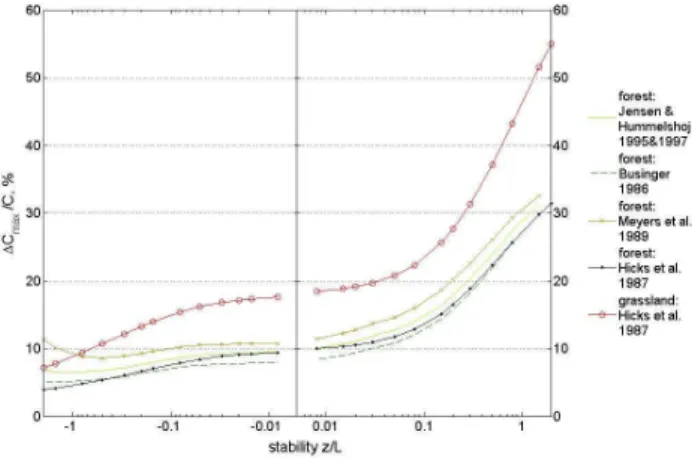
We have calculated1Cmax/Cfor a range of stabilities us-ing the roughness length (z0)and the measurement heights of the two sites using different parameterisations forRb(Fig. 2).
1Cmax/Cdepends to a large extend on the atmospheric sta-bility, ranging from 55% at the grassland site for extremely
Fig. 2. Minimal relative precision requirements (1Cmax/C in %)
assuming a maximum HNO3deposition flux (Rc=0) for a grassland
site (NEU) and a forest site (EGER). For the forest site different pa-rameterizations forRbexisting in literature (Businger, 1986; Jensen and Hummelshoj, 1995, 1997; Meyers et al., 1989) are applied.
stable conditions (32% at the forest site) to less than 10% at the grassland (around 5% at the forest site) for labile condi-tions. Higher roughness at the forest site (EGER) leads to generally lower1Cmax/Cvalues for all stabilities compared to the grassland site.
3.2 Influence of the measurement heights
The influence of the measurement heights above the surface on the minimal precision requirements is also estimated from Eq. (10). For near neutral conditions, whenz/L is close to zero,9H is close to zero such that we may simplify Eq. (10) to:
1Cmax
CHNO3 = ln z2 z1
lnz2
z0
+2· P rSc
23 (11)
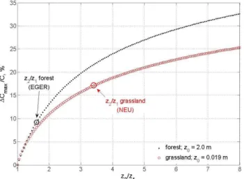
The second term in the denominator is a constant derived fromRb, which has a bigger influence on1Cmax/C above a forest than above grassland, where ln(z2/z0) is smaller.
Fig. 3. Minimal relative precision requirements (1Cmax/C in %)
for neutral stability and a range of measurement height ratiosz2/z1
for forest and grassland. Additionally indicated arez2/z1values for the sites used in this study.
4 Experimental results
4.1 Overview
The determined random error of the measured air concen-trations, determined after Trebs et al. (2004) and Thomas et al. (2009), was in the order of 10%. Note here, that only in-dividual quantifiable error sources are included in this error estimation. Errors in concentration values that are not quan-tifiable, e.g., errors due to limited sampling efficiency, may only be investigated by differential analysis, like the side-by-side measurements (see Sects. 2.2.3 and 4.2). The limit of detection (LOD) under field conditions was determined as three times the standard deviation of the blank values (Kaiser and Specker, 1956) and results are summarized in Table 1. During NEU, problems with the membrane in the FIA and sensor damage in the course of the experiment increased the LOD of the NH3/NH+4- measurement.
Concentration values below the detection limit were used in the general time series analysis, but data points were flagged and their error (σC/C) was set to 100%. However, for the side-by-side evaluation they were excluded. Further-more, data points were excluded from further analysis based on chromatogram quality, water quality, air and liquid flow stability and obvious contamination (e.g., after manual air flow measurement). An outlier test was performed according to Vickers and Mahrt (1997) and the respective values were excluded from analysis. The overall data availability during the experiments is shown in Table 2. Roughly 10% of the measurement period was used for calibrations and blanks. One third was used for side-by-side measurements and two thirds of the measurement period the instrument measured concentration at two different heights.
Table 1.Limits of detection (3σ-definition) for the gas/particle con-centrations determined under field conditions at the two campaign sites.
NEU EGER
µg m−3in air µg m−3in air
NH3/NH+4 0.055 0.074 0.021 0.022
HNO3/NO−3 0.094 0.093 0.132 0.130
4.2 Diel variation of concentrations and aerodynamic parameters
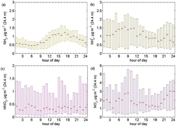
Diel variations of the concentrations measured during the ex-periments are presented in Fig. 4 (NEU) and Fig. 5 (EGER) as median, 0.25 and 0.75 percentiles. During NEU, NH3 con-centrations atz=0.37 m (above ground) (median values: 1.24 to 3 µg m−3)exceeded concentrations of all other compounds by a factor of 2 to 4 and were higher than those observed during EGER (median values: 0.46 to 1.16 µg m−3). Dur-ing NEU, NH3 concentrations featured a sharp peak during the morning hours, while NH3 peaked in the afternoon/late afternoon hours during EGER. Concentrations of particu-late NH+4 were twice as high during EGER (median values: 0.9 to 1.44 µg m−3)compared to NEU (median values: 0.31 to 0.77 µg m−3). During both campaigns, particulate NH+4 exhibited a diel variation with higher concentrations during nighttime and lower concentrations during daytime. HNO3 concentration levels were similar during NEU and EGER with median values between 0.2 and 0.7 µg m−3. No signif-icant diel variation of HNO3was observed above the forest during EGER while HNO3featured a typical diel cycle with broad maxima in the afternoon during NEU. Particulate NO−3 concentrations were much larger during EGER than during NEU, with median values between 1.8 and 3 µg m−3. Al-though, the variation of particulate NO−3 was smaller during EGER than during NEU, it typically showed highest values during nighttime and/or in the early morning hours.
The friction velocity, u∗, ranged between 0.07 and 0.23 m s−1during NEU, with highest values during the day (Fig. 6).z/Lranged from−0.25 to 0.3, indicating stable con-ditions at night and unstable and near neutral concon-ditions dur-ing the day. Durdur-ing EGER,u∗was much higher with values between 0.25 and 0.8 m s−1andz/Lwas between−0.3 and 0.5, also indicating stable conditions during nighttime and neutral/unstable conditions during daytime.
194 V. Wolff et al.: An analysis of precision requirements and flux errors
Table 2.Overview of the data availability for the two experiments (NEU, grassland, Switzerland, 2006, and EGER, forest, Germany, 2007).
SB1 and SB2: sample box one and sample box two. For the concentration differences,1C, only values with both concentration values>LOD
were used.
NEU side-by-side gradient
Tot No. <LOD No. of1C Tot No. <LOD No. of1C
σ
Δ
Δ Δ
Δ Δ
NH3 SB1 188 1% 146 612 0% 490
SB2 202 1% 515 0%
NH+4 SB1 106 35% 27 550 11% 251
SB2 90 53% 365 24%
HNO3 SB1 145 19% 91 478 18% 271
SB2 194 10% 345 7%
NO−3 SB1 108 2% 62 535 0% 316
SB2 174 3% 340 2%
EGER side-by-side gradient
Tot No. <LOD No. of1C Tot No. <LOD No. of1C
σ
Δ
Δ Δ
Δ Δ
NH3 SB1 20 4% 148 528 1% 482
SB2 184 9% 495 0%
NH+4 SB1 230 1% 198 501 1% 451
SB2 219 1% 495 2%
HNO3 SB1 216 8% 176 449 31% 284
SB2 219 19% 433 31%
NO−3 SB1 215 2% 203 486 6% 409
SB2 232 3% 454 10%
4.3 Error of1Cdetermined from side-by-side measurements
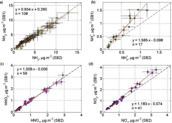
To estimate the effective error of1C(σ1C)under field con-ditions, we used results from extended side-by-side sam-pling periods during both experiments. The weather condi-tions and ambient concentracondi-tions of the compounds under study were similar during side-by-side and aerodynamic gra-dient measurements. Results from the side-by-side measure-ments are displayed as scatter plots in Figs. 7 and 8 for NEU and for EGER, respectively. Concentrations sampled during rain events and during episodes with high relative humidity (>95%) are excluded from the side-by-side evaluation and from the flux determinations, since during these times ad-sorption processes in the humid inlet and potential contam-ination of the denuder by water droplets can not entirely be excluded.
Figures 7 and 8 show marked linear correlations between concentrations measured by the two sample boxes, however, deviations from the 1:1 line and scatter around the fitted lines is visible. HNO3side-by-side measurements featured slopes with little deviation from the 1:1 line (1.01 and 1.02 for NEU and EGER, respectively) and small offsets. Side-by-side
measurements for NH3 during NEU (Fig. 7a) also featured a slope close to unity (slope: 0.93). During EGER (Fig. 8a), under much lower NH3 concentrations, the deviation from the 1:1 line was somewhat larger (1.13), whereas the offset was smaller. For the particulate compounds (NH+4 and NO−3)
the deviations from the 1:1 line are larger than for HNO3and NH3 (Fig. 7b, d and and Fig. 8b, d). The largest deviation from the 1:1 line in both experiments is observed for partic-ulate NH+4, with a slope of 1.59 in the NEU experiment and 1.31 in the EGER experiment.
After we corrected the data using the orthogonal fit (sys-tematic deviation, see above), the remaining scatter around the fit (the residuals) was used to determineσ1C. Figure 9 shows exemplarily two typical residual distributions.
Fig. 4. Diel variation of(a)NH3,(b)particulate NH+4,(c)HNO3, and(d)particulate NO−3 measured atz=0.37 m (above ground). Red
lines are median concentrations, boxes denote the inter-quartile range (0.25–0.75) during NEU in Oensingen (Switzerland), 2006 (managed grassland ecosystem).
196 V. Wolff et al.: An analysis of precision requirements and flux errors
Fig. 6.Diel variation of friction velocity (u∗) during(a)NEU and(c)EGER and of the stability (z/L) during(b)NEU and(d)EGER. Red lines denote the median, the boxes the inter-quartile ranges (0.25–0.75).
distribution is determined as:
stdLaplace= √
2· N P
i=1 |xi− ¯x|
n (12)
withndenoting the total number of values within the distri-bution,x¯the mean, andxi all residual values, which encom-pass 76% of the Laplace distribution (which corresponds to 68.27% in the Gaussian distribution, analogously, 2 std cor-respond to 95.45% of a Gaussian distribution, but to 94% of a Laplace distribution; see Richardson et al., 2006).
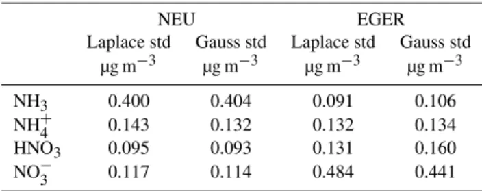
The distributions of concentration residuals provide valu-able information on the behaviour of the instrument. The width of the residual distribution characterizes the random concentration difference during side-by-side measurements in the field. The Laplace standard deviations for each of the compounds are given in Table 3 for the two experiments. For comparison, the standard deviations calculated for the Gaus-sian distribution are also shown.
For NH3, HNO3 and NO−3 during NEU and NH3, NH+4 and HNO3during EGER, we observed increasing std1C val-ues with increasingC. Therefore, we plotted std1CversusC
measured by SB2 and made a linear regression (see Figs. 10 and 11), which can be used to determine std1Cas a function ofC. The relative values std1C/C derived from the slopes of the regressions, which are used as estimates ofσ1C, are summarized in Table 4. For particulate NH+4 during NEU and for particulate NO−3during EGER, this approach did not
Table 3. Laplace and Gaussian standard deviations, std1C of the
residuals of the concentration difference obtained during the side-by-side measurements after correcting the data for systematic devi-ations using the orthogonal fit for NEU and EGER.
NEU EGER
Laplace std Gauss std Laplace std Gauss std
µg m−3 µg m−3 µg m−3 µg m−3
NH3 0.400 0.404 0.091 0.106
NH+4 0.143 0.132 0.132 0.134
HNO3 0.095 0.093 0.131 0.160
NO−3 0.117 0.114 0.484 0.441
appear to be useful, because the residuals did not show a clear dependence onCin these cases. Hence, we defined the over-all Laplace standard deviation (Table 3) as the error σ1C. Median relative determined errors (σ1C/1C) were 36.3 and 55.5% for NH3, 40.1 and 59.4% for HNO3, 129.6 and 63.3% for particulate NH+4 and 49.4 and 244% for particulate NO−3 during NEU and EGER, respectively.
Fig. 7.Results from side-by-side measurements during the NEU experiment. The error bars indicate the random errors of the concentration measurements. Red lines and the given equations represent the individual orthogonal fits. n is the number of data points used for each fit. The dashed line indicates the 1:1 line. (SB1: sample box 1; height 0.37 m; SB2: sample box 2; height 1.23 m).
198 V. Wolff et al.: An analysis of precision requirements and flux errors
(a) (b)
Fig. 9. Residuals of1Cfor side-by-side measurements after correcting the data for systematic deviations using the orthogonal fit for(a)
HNO3(EGER) and(b)NH3(NEU). The lines indicate fitted Laplace (blue) and Gaussian (red) distributions.
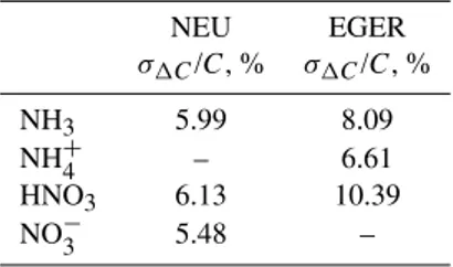
Table 4.Errors of the concentration difference, relative to the
am-bient concentration,σ1C/C, determined for NEU and EGER. For
particulate NH+4 during NEU and particulate NO−3 during EGER
only absolute values independent ofC could be determined (see
text and Table 3).
NEU EGER
σ1C/C, % σ1C/C, %
NH3 5.99 8.09
NH+4 – 6.61
HNO3 6.13 10.39
NO−3 5.48 –
are larger than1C itself and it is not possible to derive sig-nificant fluxes from these1C values, nor meaningful depo-sition velocities.
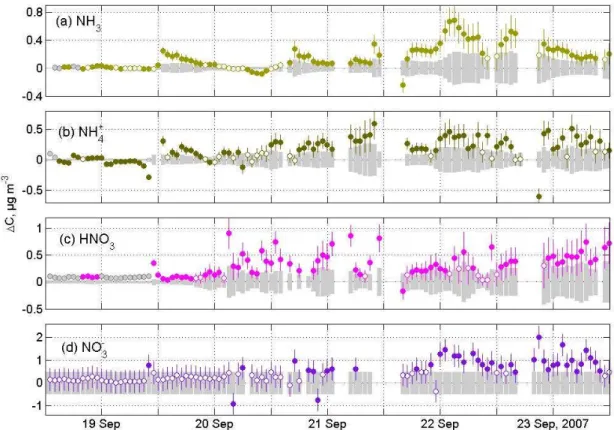
We define those 1C values as insignificantly different from zero. Results of this analysis for some days of the EGER experiment are displayed in Fig. 12. In cases when the uncertainty range is a function of concentration (NH3, NH+4, HNO3), the diel variation of concentrations is reflected in the varying size of the error bars and uncertainty ranges (grey bars). For example, for NH3 concentrations during EGER error bars are larger during daytime when NH3 concentra-tions are high (Fig. 12a). In the case of NO−3, an overall con-stant uncertainty was estimated using the Laplace standard deviation from Table 3 (see above) and is illustrated by the uniform grey uncertainty range in Fig. 12d. For the days shown here, both, significant and non-significant1Cvalues are observed.
From the relative values, σ1C/C, in Table 4 we define an uncertainty range around zero and therefore a signifi-cance level for1Cfor the given ambient concentration. Be-tween 11 to 54% of the individual1C values, determined from aerodynamic gradient measurements, during EGER and NEU are found to be significantly different from zero (Table 5).
Table 5. : Percentage of significant1C (values larger thanσ1C)
during gradient measurements for NEU and EGER.
NEU EGER
Number of significant Number of significant
1C(% of total) 1C(% of total)
NH3 263 (54%) 245 (51%)
NH+4 60 (24%) 221 (49%)
HNO3 119 (44%) 128 (45%)
NO−3 123 (39%) 43 (11%)
4.4 Error of the transfer velocity
Since the exchange flux of the considered trace gases is de-fined as the product of1C andvtr we also need to investi-gateσvtr. As stated above,vtr is a function ofu∗, and, in
the denominator, ln(z2/z1)and the integrated stability cor-rection functions for heat (= trace compounds) for both mea-surement heights (9H(z1/L) and9H(z2/L)), which are (via the Obukhov length, Eq. 2) a function ofu∗, the sensible heat flux (H), a buoyancy parameter (g/T), the air density (ρ), the von Karman constant and the specific heat (cp)(e.g., Arya 2001).
A complete error analysis of vtr would require informa-tion about the error of all these parameters. We have not found any study, which has thoroughly quantifiedσvtr. Since
a detailed analysis ofσvtris not the main scope of this study,
Fig. 10.Residuals of1Cduring side-by-side after correcting the data for systematic deviations using the orthogonal fit (individual values:
blue points) and their relation toCduring NEU. The derivedσ1Cis shown as red line (uncertainty range around zero).
Fig. 11.Residuals of1Cduring side-by-side after correcting the data for systematic deviations using the orthogonal fit (individual values:
200 V. Wolff et al.: An analysis of precision requirements and flux errors
Fig. 12. Measured1Cvalues above the spruce forest canopy for some days during EGER. Error bars and uncertainty ranges (grey bars) for(a)NH3,(b)particulate NH+4,(c)HNO3and(d)particulate NO−3 were determined from the residual analysis described in the text. The
hollow circles are values of1Cthat are statistically not significant different from zero, the filled circles are significant1Cvalues. Grey
circles are values of1Cwhere one or both concentrations were below the LOD.
For non-neutral conditions, error estimates of the empiri-cal functions within the stability range of−0.5≤z/L≤+0.5 exist (Foken, 2006). Assuming that the errors remain the same when integrating the empirical functions the errors would also be in the range of≤10%. Assuming near-normal distribution of bothσu∗andσ9H,σvtr can be calculated
ac-cording to:
σvtr
vtr=± v u u u u t
σu∗
u∗
2
+
σψH
ψH
2
·
(ψH(z2)+ψH(z1))2
ln
z2
z1
−ψH(z2)+ψH(z1)
2
(13)
The right hand term of the product under the square root accounts for the fact that in Eq. (3) two9H functions ap-pear in the denominator. Note that we assume a maximum relative error of both 9H functions (10%). The errors of
u∗ and9H add up to a daytime (−0.5≤z/L≤+0.5)σvtr/vtr
of around 10% (median) during NEU (inter-quartile range: 10.1–13.3%) and 13% (median) during EGER (inter-quartile range: 10.3–23.2%). For smallu∗values the assumption of a constant relative error may not be fully appropriate. But we use this simplified assumption here sinceu∗has no influ-ence on the sign of the flux and therefore its uncertainty is generally not limiting for the significance of the flux.
4.5 Flux error
In the previous sections we have determined σ1C/1C and we also obtained an error estimate forσvtr/vtr. We combine
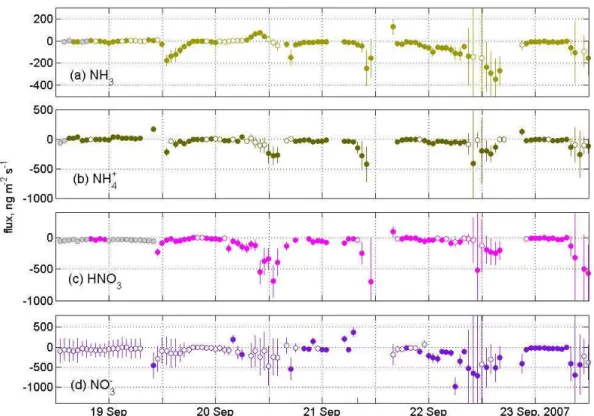
these relative errors and derive the flux error,σF, applying Eq. 4. The resultingσF are presented along with determined fluxes in Fig. 13 for some days during EGER.
Most of the timeσF is primarily governed byσ1C, but on the 22 and 23 September, largeσvtr values dominateσF
dur-ing daytime. The overallσF during EGER would decrease by 4% (median, inter-quartile range: 2–10%) if we exclude
σvtr and use σ1C only. During NEU, the error would
de-crease by 2% (median, inter-quartile range: 1–4%). It is ev-ident that, σF depends to a major extent on the capability of the instrument to precisely resolve vertical concentration differences.
Fig. 13.Fluxes of(a)NH3,(b)particulate NH+4,(c)HNO3, and(d)particulate NO−3 during EGER. Error bars are derived from both,σvtr
andσ1C. Hollow symbols denote flux values that are derived from1Cthat are insignificantly different from zero (Sect. 4.2). Grey circles
denote flux values calculated with one or both concentrations below the LOD.
σF/F vary between 31 and 68%. The values are comparable for all compounds, but show slightly larger ranges and higher medians for NH+4 during NEU and NO−3 during EGER
5 Discussion
5.1 Side-by-side performance of the GREAGOR system
As stated in Sect. 2.2.3 the error in concentration difference,
σ1C, may not be derived from the error in concentrations, as some of the factors that influenceCdo not impact on1C, but others do. The error of the peak integration, which affects the measured liquid concentration and the measured bromide concentration (cf. Trebs et al., 2004), for example, is relevant for1Cas these errors may vary during the sequential runs of the ion chromatograph. Additionally, the two airflows though the sample boxes may have slightly different variations since the two critical orifices are not entirely identical. There are also some other factors that may affect1C which are hard to quantify and to monitor. The wet-annular rotating denuder walls may not always be perfectly coated, and the liquid lev-els, controlled by optical sensors, may be slightly different between the two wet-annular rotating denuders. The differ-ence in coating quality would lead to slightly different sam-pling efficiencies between the two heights, especially if the coating is not perfect in the first part of the denuder (Thomas
et al., 2009). The difference in water level results in a dif-ferent response time of the instrument, leading to a damp-ening of concentration variations in the potentially affected denuder (Thomas et al., 2009). 1C may also be influenced by inlet effects of the two sample boxes. Due to their high solubility and high surface affinity, HNO3and NH3may be lost in the inlet, especially under very humid conditions. To minimize these effects we used short PFA tubing and treat measurement values from periods with rain and high relative humidity with caution. This, however, may not fully exclude different behaviour of the two inlets.
202 V. Wolff et al.: An analysis of precision requirements and flux errors
Fig. 14. Statistical representation of the relative flux error (σF/F)
for NH3, particulate NH+4, HNO3, and particulate NO−3 during NEU in Oensingen (Switzerland), 2006 (managed grassland
ecosys-tem). Only data derived from significant values of1Care used.
The SJACs do not reveal significant differences for higher particulate NH+4 concentrations (see Thomas et al., 2009), but discrepancies were consistently observed for ambient concentrations below 2.5 µg m−3. The deviations of up to 59% (Figs. 7 and 8) between the two sample boxes indicate that the SJAC sampling efficiency for NH+4 was not equal for the two devices. For the NEU experiment, NH+4 con-centrations were quite low (up to 2 µg m−3; compared to 14 µg m−3 in Thomas et al., 2009) and the regression was calculated for 17 data pairs only (Fig. 7). Deviations for particulate NH+4 using the denuder SJAC sampling devices were observed also by other scientists using the MARGA system (R. Otjes, personal communication, 2009). It was hypothesised that bacteria were captured and subsequently retained by the walls of one of the SJACs, leading to a con-version of N-containing species (with a preference for NH+4). This assumption is supported by the better comparability of our side-by-side measurements for particulate NO−3 (Figs. 7d and 8d) and SO24− (not shown). The addition of hydrogen peroxide to the absorption solutions of the MARGA solved this problem (R. Otjes, personal communication, 2009). We conclude that GAEGOR may also have suffered from such a bacterial infection during our studies. Since the differences proved to be quite stable during both experiments, we were able to correct for this systematic difference (cf. Sect. 2.2.3). 5.1.1 Overview of NH3-HNO3-NH4NO3aerodynamic
gradient measurements
Table 6 shows a list of studies that have measured and in-vestigated vertical concentration gradients of NH3, HNO3 and particulate NH+4/NO−3 to determine surface-atmosphere exchange fluxes over different ecosystems, focussing on multi-component gradient measurements (only a few single-compound measurements were included). Especially for NH3this table is not complete.
Fig. 15. Statistical representation of the relative flux error (σF/F)
for NH3, particulate NH+4, HNO3, and particulate NO−3 during
EGER in Waldstein (Germany), 2007 (spruce forest ecosystem).
Only data derived from significant values of1Care used.
Table 6.List of studies that have performed aerodynamic gradient measurements of NH3, HNO3, particulate NH+4/NO−3. Indicated are the
measured species, whether or not the method was continuous or semi-continuous, and whether a precision (error) estimate was used to derive and discuss exchange fluxes.
NH3 HNO3 NH+4 NO−3 continuous/ Flux error
semi-continuous estimate
(1) (Huebert and Robert, 1985)
(2) (Erisman et al., 1988)
(3) (Duyzer et al., 1992)
(4) (Wyers et al., 1992)
(5) (Andersen et al., 1993)
(6) (Erisman and Wyers, 1993)
(7) (Duyzer, 1994)
(8) (Sievering et al., 1994)
(9) (Andersen and Hovmand, 1995)
(10) (Wyers and Duyzer, 1997)
(11) (Flechard and Fowler, 1998)
(12) (Van Oss et al., 1998)
(13) (Wyers and Erisman, 1998)
(14) (Andersen et al., 1999)
(15) (Nemitz et al., 2000)
(16) (Sutton et al., 2000b)
(17) (Milford et al., 2001)
(18) (Rattray and Sievering, 2001)
(19) (Sievering et al., 2001)
(20) (Spindler et al., 2001)
(21) (Pryor et al., 2002)
(22) (Nemitz et al., 2004a)
(23) (Nemitz et al., 2004b)
(24) (Nemitz and Sutton, 2004)
(25) (Phillips et al., 2004)
(26) (Kruit et al., 2007)
(27) (Thomas et al., 2009)
5.1.2 Error of concentration differences
About 49% of1C data for NH3 during EGER were found to be not significantly different from zero (Table 5). Keeping in mind that measurements were performed above forest with the expected small1Cvalues (Fig. 3), a 51% yield of signifi-cant half hourly aerodynamic gradient measurements is satis-fying. Andersen et al. (1993), who measured NH3exchange with three hourly-integrated denuder measurements on sev-eral levels above forest, were able to use less than half of the measurements for flux calculations. Wet-chemical semi-continuous methods comparable to GRAEGOR, for which the precision to resolve vertical concentration differences was determined have been presented by Wyers et al. (1993), Kruit et al. (2007), and Thomas et al. (2009). Wyers et
204 V. Wolff et al.: An analysis of precision requirements and flux errors conditions, feeding the three wet-annular rotating denuders
simultaneously with two different standard NH3 concentra-tions (0 and 8 µg m−3)over five hours and corrected for the deviations between the samples in the same way as Wyers et al. (1993) (see Sect. 4.1.1). From these tests, they conclude that their precision was at least as good as found by Wyers et al. (1993), if not better (<1.9%). However, these tests do neither take into account the behaviour of the measurement system and analytical unit under ambient conditions nor the dynamic changes of ambient concentrations and associated fluctuations of temperature and relative humidity during field experiments.
In 2009, Thomas et al. (2009) introduced the GRAEGOR instrument and investigated its precision by performing a side-by-side experiment in the field under ambient condi-tions. They calculated linear regressions through the con-centration data and used the deviation of the derived slope from the 1:1 line as their precision. They found 3% for gases and 9% for particulate compounds. The use of the de-viation from the 1:1 line as precision estimate (not taking into account the scatter around it) is different to the meth-ods used by Wyers et al. (1993) and Kruit et al. (2007), who defined this a systematic error and derived their random er-ror from the remaining scatter. However, the approach by Thomas et al. (2009) was a first attempt to estimate the in-strument precision for aerodynamic gradient measurements. Thomas et al. (2009) also defined their minimum detectable flux whenσ1Cequals1C, but they did not take into account the error of the transfer velocity. Side-by-side measurements by Thomas et al. (2009) featured smaller systematic devi-ations from the 1:1 line than found in our study. Concen-tration ranges for NH3, HNO3and NO−3 are comparable to the ones observed in our experiments, while particulate NH+4 presented in Thomas et al. (2009) reached 14 µg m−3, which is more than 3 times of our NH+4 concentrations. Differ-ences in the performance of the sample boxes may be due to small changes in the set up as well as the use of differ-ent wet-annular rotating denuder or SJAC couples. It may also be strongly influenced by environmental conditions (see Sect. 5.1). An analysis of the Thomas et al. (2009) side-by-side data with our method results inσ1C/C median values of 4.5% for NH3, 1.0% for NH+4, 4.6% for HNO3, and 6.8% for NO−3. These values are lower than the ones found in our study (see Table 4) especially for particulate NH+4, which however revealed much higher concentrations in Thomas et al. (2009). In this study, we combined the approaches of Wyers et al. (1993), Kruit et al. (2007), and Thomas et al. (2009) by separating systematic from random effects us-ing the scatter around the fitted line and by usus-ing side-by-side measurements in the field to account for the actual set up of the instrument and the environmental conditions encountered at the field sites. A difference to the previous studies is the use of an orthogonal fit rather than a least squares regres-sion to evaluate the side-by-side measurements. This fit takes
into account that concentration measurements of both sample boxes may be erroneous, which is a more realistic approach than defining one of the measurements as independent (Ay-ers, 2001; Cantrell, 2008; Hirsch and Gilroy, 1984). The median σ1C/1C values range between 36% (NH3 during NEU) and 244% (NO−3 during EGER), see Sect. 4.2. Keep-ing in mind, that the GRAEGOR is a semi-continuous mea-surement device, delivering all compounds of the triad (and more) in hourly resolution and that we use in-field data rather than laboratory test to express an field precision of the in-strument, these precision values are certainly satisfying. 5.1.3 Error of surface exchange fluxes
There are only six studies that show and discuss error bars of fluxes derived from measurements applying the AGM (see Table 6). Erismann and Wyers (1993) discussed in their study on SO2and NH3exchange fluxes above forest that the main error source for the NH3flux and the NH3canopy resistance error isσ1C. They show data of NH3fluxes and correspond-ingRcvalues with error bars of up to 100% and higher. They suggested an error weighted approach when doing time se-ries analysis of these data.
Thomas et al. (2009) show a figure with flux data carrying flux errors. The magnitude relative to the flux value is not discussed in detail but is estimated well within±50%. The same relative value is true for flux errors shown in a figure from Duyzer et al. (1994). All these errors do not include
σvtr.
The relative flux errorsσF/F determined in our study, with medians between 31 and 68% (see Figs. 14 and 15), are com-parable to these studies.
5.2 Influence of stability conditions on the precision
In Sect. 3.1 we investigated the expected magnitude of1C
for a range of atmospheric stabilities, assuming a maximum HNO3deposition flux. The precision requirement is higher for the forest site (EGER) with around 10% for near neutral and less than 10% for unstable conditions. These estimates depend to a major extend on the applied parameterisation for
Rb (see Fig. 2). Comparing these values with the relative precision values given in Table 4 (EGER: right side) we see that for some species the precision may not be sufficient to determine significant1Cabove the forest for all atmospheric stabilities.
5.3 Influence of measurement height on the precision
It is evident from Sect. 3.2, which impact the choice of the measurement heights has on the required1Cto be resolved. Knowing the relative precision of the instrument, for exam-ple 8% for NH3 during EGER, minimal z2/z1 ratios to re-solve differences above a surface of given roughness can be calculated. However, as it was the case for the studies con-ducted here, the measurement heights must be adjusted to micrometeorological considerations (such as uniform fetch length).
6 Conclusions
In this paper we made a comprehensive precision analysis for a novel wet-chemical instrument used for aerodynamic gra-dient measurements of water-soluble reactive trace gases and particles (GRAEGOR; GRadient of AErosol and Gases On-line Registrator; ECN, Petten, NL) with focus on the NH3 -HNO3-NH4NO3triad. For the first time, we present a thor-ough determination of errors of multi-component surface-atmosphere exchange fluxes for two contrasting ecosys-tems (managed grassland and spruce forest). From our in-vestigations, we draw conclusions on the significance of measured concentration differences and, thus, the direction and magnitude of multi-component surface-atmosphere ex-change fluxes.
Additionally, we investigated theoretical minimal preci-sion requirements for surfaces with different roughness with regard to atmospheric stability and measurement heights, which may be used for future experimental designs, know-ing the precision of the instrument that will be used. Derived in-field precision values (σ1C/C) of the instrument during our field studies were 6% (NEU, grassland) and 8% (EGER, forest) for NH3, 6% (NEU) and 10% (EGER) for HNO3, and 7% for particulate NH+4 (EGER) and 5% for particu-late NO−3 (NEU). Thus, GRAEGOR is capable of resolv-ing vertical concentration differences of the four species un-der investigation above grassland and forest sites for most of the prevailing atmospheric stabilities. However, our analy-sis revealed that, especially at the forest site, the precision of the instrument may not be sufficient to resolve individual (hourly) gradients at labile atmospheric stability, even if the substance is deposited at maximum possible speed.
Despite the fact that GRAEGOR is operated using the same analytical device for both measurement heights the me-dian error of the determined concentration difference ranges between 36 and more than 100%. The individual errors that lead to these uncertainties are hard to quantify under field conditions. However, the determination of the limit of detection and side-by-side measurements under field con-ditions are a suitable tool to evaluate the instrument per-formance and to estimate the instrument precision and as-sociated flux errors. The precision of GRAEGOR may be
improved by intensive monitoring and controlling of error sources for aerodynamic gradient measurements like denuder liquid level and sample efficiency of the SJACs. We may as-sume that errors in previous studies, where the aerodynamic gradient method was used to derive exchange fluxes of the NH3-HNO3-NH4NO3 triad, were at least as high as during our study, especially if two different analytical devices were applied.
The instrument provides a semi-continuous data set, con-stituting valuable information for mechanistic process stud-ies. Our results form the basis to explore the errors of de-position velocities and canopy compensation point concen-tration, which are key-parameters used in all atmospheric chemistry and transport models. The results from the NEU and EGER campaigns will be discussed and interpreted in separate publications.
Acknowledgements. The authors gratefully acknowledge financial
support by the European Commission (NitroEurope-IP, project 017841), the German Science foundation (DFG project EGER, ME 2100/4-1) and by the Max Planck Society. The authors wish to thank the Agroscope Reckenholz-T¨anikon Research Station (ART, Air Pollution and Climate Research Group) for hosting us during the NitroEurope study and the University of Bayreuth (Mi-crometeorology Department) for hosting us during the EGER study.
The service charges for this open access publication have been covered by the Max Planck Society.
Edited by: M. Weber
References
Alsheimer, M.: Charakterisierung r¨aumlicher und zeitlicher Het-erogenit¨aten der Transpiration unterschiedlicher montaner Ficht-enbest¨ande durch Xylemflussmessungen, Bayreuther Forum
¨
Okologie, 1–143, 1997.
Ammann, C.: On the Applicability of Relaxed Eddy Accumulation and Common Methods for Measuring for Measuring Trace Gas Fluxes, PhD thesis, ETH, Z¨urich, 1998.
Ammann, C., Flechard, C. R., Leifeld, J., Neftel, A., and Fuhrer, J.: The carbon budget of newly established temperate grassland depends on management intensity, Agr. Ecosyst. Environ., 121, 5–20, 2007.
Andersen, H. V. and Hovmand, M. F.: Ammonia and nitric acid dry deposition and throughfall, Water Air Soil Poll., 85, 2211–2216, 1995.
Andersen, H. V., Hovmand, M. F., Hummelshoj, P., and Jensen, N. O.: Measurements of Ammonia Flux to a Spruce Stand in Denmark, Atmos. Environ. A-Gen., 27, 189–202, 1993. Andersen, H. V., Hovmand, M. F., Hummelshoj, P., and Jensen, N.
O.: Measurements of ammonia concentrations, fluxes and dry deposition velocities to a spruce forest 1991–1995, Atmos. Env-iron., 33, 1367–1383, 1999.
Arya, S. P.: Introduction to Micrometeorology, Academic Press, Cornwall, UK, 420 pp., 2001.
206 V. Wolff et al.: An analysis of precision requirements and flux errors
Brodeur, J. J., Warland, J. S., Staebler, R. M., and Wagner-Riddle, C.: Technical note: Laboratory evaluation of a tunable diode laser system for eddy covariance measurements of ammonia flux, Agr. Forest Meteorol., 149, 385–391, 2009.
Businger, J. A.: Evaluation of the Accuracy with Which Dry Depo-sition Can Be Measured with Current Micrometeorological Tech-niques, J. Clim. Appl. Meteorol., 25, 1100–1124, 1986. Businger, J. A. and Delany, A. C.: Chemical Sensor Resolution
Required for Measuring Surface Fluxes by 3 Common Microm-eteorological Techniques, J. Atmos. Chem., 10, 399–410, 1990. Calvert, J. G., Lazrus, A., Kok, G. L., Heikes, B. G., Walega, J.
G., Lind, J., and Cantrell, C. A.: Chemical Mechanisms of Acid Generation in the Troposphere, Nature, 317, 27–35, 1985. Cantrell, C. A.: Technical Note: Review of methods for linear
least-squares fitting of data and application to atmospheric chemistry problems, Atmos. Chem. Phys., 8, 5477–5487, 2008,
http://www.atmos-chem-phys.net/8/5477/2008/.
Cape, J. N., van der Eerden, L. J., Sheppard, L. J., Leith, I. D., and Sutton, M. A.: Evidence for changing the critical level for ammonia, Environ. Pollut., 157, 1033–1037, 2009.
Cellier, P. and Brunet, Y.: Flux Gradient Relationships above Tall Plant Canopies, Agr. Forest Meteorol., 58, 93–117, 1992. Duyzer, J.: Dry Deposition of Ammonia and Ammonium Aerosols
over Heathland, J. Geophys. Res.-Atmos., 99, 18757–18763, 1994.
Duyzer, J. H., Verhagen, H. L. M., Weststrate, J. H., and Bosveld, F.
C.: Measurement of the dry deposition flux of NH3on to
conif-erous forest, Environ. Pollut., 75, 3–13, 1992.
Erisman, J. W., Bleeker, A., Hensen, A., and Vermeulen, A.: Agri-cultural air quality in Europe and the future perspectives, Atmos. Environ., 42, 3209—3217, 2008.
Erisman, J. W., Draaijers, G., Duyzer, J., Hofschreuder, P., Van-Leeuwen, N., Romer, F., Ruijgrok, W., Wyers, P., and Gallagher, M.: Particle deposition to forests - Summary of results and ap-plication, Atmos. Environ., 31, 321–332, 1997.
Erisman, J. W. and Schaap, M.: The need for ammonia abatement with respect to secondary PM reductions in Europe, Environ. Pollut., 129, 159–163, 2004.
Erisman, J. W., Vermetten, A. W. M., Asman, W. A. H., Wai-jersijpelaan, A., and Slanina, J.: Vertical-Distribution of Gases and Aerosols – the Behavior of Ammonia and Related Com-ponents in the Lower Atmosphere, Atmos. Environ., 22, 1153– 1160, 1988.
Erisman, J. W. and Wyers, G. P.: Continuous Measurements of
Sur-face Exchange of SO2and NH3– Implications for Their Possible
Interaction in the Deposition Process, Atmos. Environ. A-Gen., 27, 1937–1949, 1993.
Falge, E., Reth, S., Bruggemann, N., Butterbach-Bahl, K., Gold-berg, V., Oltchev, A., Schaaf, S., Spindler, G., Stiller, B., Queck, R., Kostner, B., and Bernhofer, C.: Comparison of surface en-ergy exchange models with eddy flux data in forest and grassland ecosystems of Germany, Ecol. Model., 188, 174–216, 2005. Farmer, D. K., Wooldridge, P. J., and Cohen, R. C.:
Applica-tion of thermal-dissociaApplica-tion laser induced fluorescence (TD-LIF)
to measurement of HNO3, 6alkyl nitrates, 6peroxy nitrates,
and NO2fluxes using eddy covariance, Atmos. Chem. Phys., 6,
3471–3486, 2006,
http://www.atmos-chem-phys.net/6/3471/2006/.
Flechard, C. R. and Fowler, D.: Atmospheric ammonia at a moor-land site. II: Long-term surface-atmosphere micrometeorological flux measurements, Q. J. Roy. Meteor. Soc., 124, 759–791, 1998. Flechard, C. R., Neftel, A., Jocher, M., Ammann, C., and Fuhrer,
J.: Bi-directional soil/atmosphere N2O exchange over two mown
grassland systems with contrasting management practices, Glob. Change Biol., 11, 2114–2127, 2005.
Foken, T.: Lufthygienisch-bioklimatische Kennzeichnung des
oberen Egertales (Fichtelgebirge bis Karlovy Vary), Bayreuther
Forum ¨Okologie, 1–70, 2003.
Foken, T.: Angewandte Meteorologie, Springer, Heidelberg, Ger-many, 2006.
Galloway, J. N., Dentener, F. J., Capone, D. G., Boyer, E. W., Howarth, R. W., Seitzinger, S. P., Asner, G. P., Cleveland, C. C., Green, P. A., Holland, E. A., Karl, D. M., Michaels, A. F., Porter, J. H., Townsend, A. R., and Vorosmarty, C. J.: Nitrogen cycles: past, present, and future, Biogeochemistry, 70, 153–226, 2004.
Garland, J. A.: The dry deposition of sulphur dioxide to land and water surfaces, P. R. Soc. London, Proc. R. Soc. Lon. Ser. A., 354, 245–268, 1977.
Garratt, J. R.: Flux Profile Relations above Tall Vegetation, Q. J. Roy. Meteor. Soc., 104, 199–211, 1978.
Garratt, J. R.: The Atmospheric Boundary Layer, Cambridge Uni-versity Press, Cambridge, 316 pp., 1992.
Hanson, P. J. and Lindberg, S. E.: Dry deposition of reactive nitro-gen compounds: A review of leaf, canopy and non-foliar mea-surements, Atmos. Environ. A.-Gen., 25, 1615–1634, 1991. Held, A. and Klemm, O.: Direct measurement of turbulent
parti-cle exchange with a twin CPC eddy covariance system, Atmos. Environ., 40, S92–S102, 2006.
Hicks, B. B., Baldocchi, D. D., Meyers, T. P., Hosker, R. P., and Matt, D. R.: A Preliminary Multiple Resistance Routine for De-riving Dry Deposition Velocities from Measured Quantities, Wa-ter Air Soil Poll., 36, 311–330, 1987.
Hirsch, R. M. and Gilroy, E. J.: Methods of Fitting a Straight-Line to Data – Examples in Water-Resources, Water Resour. Bull., 20, 705–711, 1984.
H¨ogstr¨om, U.: Analysis of Turbulence Structure in the Surface-Layer with a Modified Similarity Formulation for near Neutral Conditions, J. Atmos. Sci., 47, 1949–1972, 1990.
Huebert, B. J. and Robert, C. H.: The Dry Deposition of Nitric-Acid to Grass, J. Geophys. Res.-Atmos., 90, 2085–2090, 1985. Huey, L. G.: Measurement of trace atmospheric species by
chemi-cal ionization mass spectrometry: Speciation of reactive nitrogen and future directions, Mass Spectrom. Rev., 26, 166–184, 2007. Jaeggi, M., Ammann, C., Neftel, A., and Fuhrer, J.: Environmental
control of profiles of ozone concentration in a grassland canopy, Atmos. Environ., 40, 5496–5507, 2006.
Jensen, N. O. and Hummelshoj, P.: Derivation of Canopy Resis-tance for Water-Vapor Fluxes over a Spruce Forest, Using a New Technique for the Viscous Sublayer Resistance, Agr. Forest Me-teorol., 73, 339–352, 1995.
Jensen, N. O. and Hummelshoj, P.: Derivation of canopy resistance for water vapor fluxes over a spruce forest, using a new technique for the viscous sublayer resistance (vol 73, p. 339, 1995), Agr. Forest Meteorol., 85, 289–289, 1997.