Geospatial Analysis of Extreme Weather Events in
Nigeria (1985 -2015) Using Self Organizing Maps
Geospatial Analysis of Extreme Weather Events
in Nigeria (1985 -2015) Using Self Organizing
Geospatial Exploration of Extreme Weather Events
A case study of precipitation in Nigeria between 1979 and 2016
Dissertation supervised by
Professor Roberto Henriques, PhD
Professor Ana Cristina Costa, PhD
Professor Jorge Mateu, PhD
February 2017
ACKNOWLEDGMENTS
I would like to express my profound gratitude to God, the giver and sustainer of life
for the privilege of life and a sound mind. I am grateful to the consortium of the
master’s program in Geospatial Technologies for funding my studies cumulating to
this dissertation. My acknowledgement wouldn’t be complete without the mention of
my wife, Temitayo Ogunjirnrin who patiently stood by me during the course of my
study in Europe. I love you baby. Finally, to family, friends and mentors, I appreciate
your contribution to my success.
Geospatial analysis of extreme weather events in Nigeria (1985–
2015) using Self Organizing Maps
ABSTRACT
The explosion of data in the information age has provided an opportunity to explore
the possibility of characterizing the climate patterns using data mining techniques.
Nigeria has a unique tropical climate with two precipitation regimes: low
precipitation in the north leading to aridity and desertification, and high precipitation
in parts of the south west and south east leading to large scale flooding. In this
research, four indices have been used to characterize the intensity, frequency and
amount of rainfall over Nigeria. A type of Artificial Neural Network called Self
Organizing Map has been used to reduce the multiplicity of dimensions and produce
four unique zones characterizing extreme precipitation conditions in Nigeria. This
approach allowed for the assessment of spatial and temporal patterns in extreme
precipitation in the last three decades. Precipitation properties for each cluster are
discussed. The cluster spatially closest to the Atlantic has high values of precipitation
intensity, frequency and duration, whereas the cluster spatially closest to the Sahara
Desert has low values. A significant increasing trend has been observed in the
frequency of rainy days in the northern region of Nigeria.
KEYWORDS
Self Organizing Maps
Extreme Climate
Precipitation
Nigeria
SUBMISSION
Submission Resulting from this Thesis
Paper
Akande, A., Costa, A., Mateu, J. & Henriques, R. (2017). Geospatial Analysis of
Extreme Weather Events in Nigeria (1985 – 2015) using Self Organizing Maps.
Advances in Meteorology, 2017.
ACRONYMS
BMU
Best Matching Unit
CA Cluster
Analysis
CHIRPS
Climate Harzards Group Infrared Precipitation with Stations
ETCCDI
Expert Team on Climate Change Detection and Indices
IDW
Inverse Distance Weighting
ITD Inter-Tropical
Discontinuity
NETCDF
Network Common Data Format
SDII
Simple Daily Intensity Index
SOM
Self Organizing Maps
TFLN
Time Lagged Feedforward Network
R1
Number of Wet Days
Rx1D
Maximum 1-Day Precipitation
INDEX OF THE TEXT
ACKNOWLEDGMENTS ... iii
ABSTRACT ... iv
KEYWORDS ... v
SUBMISSION ... vi
ACRONYMS ... vii
INDEX OF FIGURES ... ix
INDEX OF TABLES ... x
1 Introduction ... 1
2 Materials and methods ... 3
2.1 Study area ... 32.2 Data ... 4
2.2.1 Data preparation and pre‐processing... 4
2.3 Methodology ... 5
3 Results and discussion ... 7
3.1 Exploratory analysis ... 73.2 GeoSOM results ... 9
3.2.1 Outlier analysis ... 9
3.2.2 Spatial trends ... 11
3.2.3 Temporal trends ... 12
4 Conclusion ... 13
5 References ... 14
6 Appendix ... 16
INDEX OF FIGURES
Figure 1: Study area in Nigeria ... 3
Figure 2: Temporal variation of mean index values over Nigeria from 1985 to 2015 .. 8
Figure 3: Data posting of indices values from 2002 ... 9
Figure 4: U-matrix (top), boxplot (middle) and map (bottom) of the four precipitation
indices showing outliers in red in 2003 ... 10
Figure 5: Precipitation indices clustering over Nigeria in 2003 ... 12
Figure 6:Observed values of the Mann-Kendall’s test statistic ZS ... 12
INDEX OF TABLES
Table 1: Summary of rainfall indices used in the study (a wet day is defined as a day
with at least 1 mm of precipitation) ... 4
Table 2: Values of the parameters used to implement the GeoSOM algorithm ... 6
Table 3: Summary statistics of the precipitation indices for the period 1985 – 2015 ... 7
Table 4: Correlation matrix of the precipitation indices for the period 1985 – 2015 .... 7
1
Introduction
One of the visible impacts of climate change and climate variability are extreme weather events that occur from time to time in several parts of the globe. A climate extreme is “the occurrence of a value of a weather or climate variable above (or below) a threshold value near the upper (or lower) ends of the range of observed values of the variable” (IPCC 2012). Climate extremes can result in changes in the frequency, intensity, spatial extent, duration and timing of climatic phenomena. There is a growing global concern that anthropogenic activities are a major cause of the variability in the intensity and frequency of weather and climate extremes (Klein Tank, Zwiers, and Zhang 2009) (IPCC 2007) (Stefan 2005). However, it can also be argued that climate extremes are just a part of decadal global climate cycle and variability (IPCC 2014).
Climate extremes, including the ones related to precipitation, can be analyzed using several approaches (Gorricha, Lobo, and Costa 2013) (Jones et al. 2014) (Thibaud, Mutzner, and Davison 2013). The use of indices to characterize the frequency, intensity and duration of precipitation extremes is one of the ways to assess them (Alexander et al. 2006) (Donat et al. 2013) (Moberg et al. 2006) (Van den Besselaar, Klein Tank, and Buishand 2013). The joint working group CCI/CLIVAR/JCOMM Expert Team on Climate Change Detection and Indices (ETCCDI)1 has 27 standardized and recommended
climate extreme indices (Klein Tank, Zwiers, and Zhang 2009; T. C. Peterson 2005; Karl, Nicholls, and Ghazi 1999; Thomas C Peterson et al. 2001). This set of indices includes both temperature and precipitation indices.
Precipitation is one of the most important climatic parameters responsible for flood and drought in several vulnerable parts of the world. According to (IPCC 2012), there is a high chance that the frequency of heavy precipitation and total precipitation will increase in several parts of the globe in the 21st century. Evidence of climate change in Nigeria has been discussed by (Akpodiogaga- and Odjugo
2009), who reported increasing damages caused by wind and rainstorms, which are projected to increase in southern regions (Abiodun et al. 2013) The northern part of the country has been experiencing a reduction in rainfall, and an increase in the rates of dryness and heat(Obioha 2008; Onyekuru and Marchant 2014), while the rainfall amounts have been increasing in the southern part with an irregular pattern (Onyekuru and Marchant 2014; Ta et al. 2016). Moreover, climate projections for the 21st century show a significant increase of temperature over all the ecological zones (Abiodun et
al. 2013) which may have negative impacts on agriculture and food security. (Adejuwon 2006) evaluated how crop yield might respond to climate change in Nigeria, and (Enete and Amusa 2010) discuss the challenges of agricultural adaptation to climate change.
Proper study of climate extremes depends on the quality and quantity of data, as well as on how rigorously they are analyzed (IPCC 2012). When dealing with precipitation extremes, it is important to consider their synoptic aspects and dimensions. The recent increase of data from ground observations, satellites, as well as numerical models, enables the opportunity for exploring the use of data mining techniques in climatic studies (Gorricha, Lobo, and Costa 2013). One of such techniques is Cluster Analysis (CA). The use of CA to gain insight from geographical data had more serious adoption since
the 1990s decade (Xiaofeng Gong and Richman 1995). Several attempts have been made in the past to characterize extreme climate using machine learning methods. Self-Organizing Maps (SOM) have successfully been applied to several climate research including the analysis of atmospheric circulations variability (Res, Hewitson, and Crane 2002), time evolution of seasonal climate (Jr et al. 2004), climate model downscaling (Hewitson and Crane 2005), and to access to access the stationary of global climate models (Hewitson and Crane 2006).
Rodrigues (Rodrigues 2010) did a study on the spatial and temporal variation of extreme weather in the Iberian Peninsula using seven different temperature and precipitation indices. Using geostatistics, these indices were analyzed and Inverse Distance Weighting (IDW) maps were produced to compare the spatial and temporal surface distribution of the indices. Clustering was thereafter done using SOM to study areas with similar climatic characteristics for two time periods, 1951 – 1980 and 1981 – 2010. The SOM analysis were done separately for temperature and precipitation indices as mixing both indices together did not provide consistent conclusions in the Iberian Peninsula. (Gorricha, Lobo, and Costa 2013) also visualized extreme climate conditions using linear models (ordinary kriging and ordinary cokriging) and a non-linear model (a three-dimensional SOM). They made use of indices calculated from precipitation data obtained between 1998 and 2000 from nineteen meteorological station covering Madeira Island in Portugal.
Nigeria has had its fair share of climate extremes in recent times. The floods of July 10, 2011 in Lagos, August 26, 2011 in Ibadan and more recently nationwide floods of 2012 are all pointers to the extreme precipitation being experienced in the country (Okoloye et al. 2013). In Nigeria, making use of nine indices, (Gbode, Akinsanola, and Ajayi 2015) were able to study climate extremes over Kano making use of temperature and precipitation data. Using temperature data, the authors could notice a warming trend characterized by an increase in the number of warm days and warm spell. The rainfall data showed a similar increase in the amount of rainfall over the region. Other studies have attempted to use linear approaches to study temperature and rainfall trends over various parts of the country (Ekpoh and Nsa 2011), (Akinsanola 2014), (Ogungbenro and Morakinyo 2014). However, none of these studies have attempted to study their spatial local patterns. A first attempt to use data mining techniques in climatic studies of Nigeria was carried out by (Olaiya and Adeyemo 2012). Making use of a Time Lagged Feedforward Network (TFLN) and recurrent network, they could predict the future values of 8 climatic parameters.
This study will however be focused on the geoexploration of climate extremes as opposed to its prediction. Based on the framework proposed by (Gorricha, Lobo, and Costa 2013), this research will be making use of a SOM to visualize the phenomenon from a global perspective.
The atmosphere is a continuum and SOM aids the visualization of this continuum by placing very different atmospheric states on distant nodes and similar atmospheric nodes on adjacent nodes.
The objective of this research is to cluster precipitation extreme over Nigeria, characterize regions of similar precipitation patterns and characterize its evolution over a period of 31 years. Our study area is first introduced with emphasis on its climate to give a background on the type of climate we are working with. CHIRPS dataset is subsequently introduced as the precipitation data from which
precipitation extreme indices are calculated. The methodology used for this research is explained and results obtained is laid out. We wrap up this paper with a conclusion.
2
Materials and methods
2.1 Study area
Nigeria is a country located in West Africa. It lies between 40N and 140N latitude and 40E and 140E
longitude and is bordered in the South by the Atlantic Ocean and the North by the Sahara Desert (Figure 1). This gives the country a very wide range of Climatic pattern experienced throughout the year.
Figure 1: Study area in Nigeria
Its weather system is controlled by the Inter-Tropical Discontinuity (ITD). The ITD is the area of lowest pressure over West Africa separating the moist Southwest Monsoon from the Atlantic Ocean and the dry Northeast trade winds from the Sahara Desert. Hence, the ITD can be located with the aid of a change in wind direction as well as the amount of moisture in the atmosphere. This is also given by the dew point temperature. The south of the ITD usually has a dew point temperature greater than 150C
while the north of the ITD usually has a dew point temperature greater than 150C. The atmosphere to
the south of the ITD is usually moist aiding the formation of clouds at low altitude including fog while the atmosphere to the north of the ITD is usually dry and dusty preventing the formation of clouds except altocumulus and cirrus at high level.
The movement of the ITD controls the weather systems in Nigeria. It has three unique overlapping movements throughout the year; an annual movement which follows the path of the sun and is responsible for seasons, a diurnal movement consisting of a slight southward shift in the morning and a slight northward shift in the afternoon and intermediate movements observed during the northern hemisphere winter months.
According to the Koppen climate classification (Kottek et al. 2006), Nigeria has four climatic zones; the Warm desert climate in the northeast, the Warm semi-arid climate in the other parts of the north, the Monsoon climate in the Niger Delta and the Tropical savanna climate in the middle belt and parts of the south west. The main ecological zones in Nigeria are the tropical rainforest in the south, savannah in the middle belt and semi-arid zones in the North.
2.2 Data
A set of high resolution reanalysis climatic daily data from the Climate Hazards Group Infrared Precipitation with Stations (CHIRPS) from 1985 to 2015 covering our study area will be used2. CHIRPS is a quasi-global (500S – 500N) satellite and observation based precipitation estimates over land. It is a 0.05 degree resolution (about 5.5 kilometres) gridded dataset (C. C. Funk et al. 2014). Reanalysis data, unlike conventional data, provides a more wholesome look at global climatic circulation and can be used as an alternative to ground observation data (Dee et al. 2011). The data comes in the Network Common Data Form (NetCDF) format and will be manipulated using Matlab®, Microsoft Excel® and ArcGIS® software. The Network Common Data Form (NetCDF) is a file format for storing multidimensional scientific data (variables) such as temperature, humidity, rainfall etc. This data was obtained online from the Climate Hazards Group InfraRed Precipitation with Station data (CHIRPS) (ftp://chg-ftpout.geog.ucsb.edu/pub/org/chg/products/CHIRPS-2.0/; accessed: September, 2016). For details, see (C. Funk et al. 2015)
This research utilized four of the precipitation indices as defined by ETCCDI (Table 1). This is because each of the indices, by itself, shows only a part of the problem (Karl, Nicholls, and Ghazi 1999; Thomas C Peterson et al. 2001). We hope the four selected are able to achieve a global characterization of precipitation in its different perspectives (Gorricha, Lobo, and Costa 2013). By global characterization, we are referring to their ability to capture changes in amount, frequency and intensity.
Table 1: Summary of rainfall indices used in the study (a wet day is defined as a day with at least 1 mm of precipitation)
Index Descriptive name Definition Units
R1 Number of wet days Frequency of rainy days days
Rx1d Maximum 1-day precipitation Maximum 1-day precipitation mm
SDII Simple Daily Intensity Index Ratio between the total rain on wet days and the number of wet days mm/day
Rx5d Maximum 5-day precipitation Highest consecutive 5-day precipitation mm
2.2.1 Data preparation and pre-processing
The representation and quality of data is very important in determining the quality of clusters that will be seen (Kotsiantis, Kanellopoulos, and Pintelas 2006). Hence, there is a need to do some amount of pre-processing to the data before clustering. Given that we are making use of a gridded reanalysis data,
we expect to have a consistent and coherent data without outliers or missing values. For this research, several data preparatory tasks were carried out prior to actual analysis, including:
Dimensionality Reduction: Out of the several temperature and precipitation indices defined by ETCCDI to characterise climate extremes, four precipitation indices (Table 1) were selected based on previous studies by (Gorricha, Lobo, and Costa 2013) and expert opinion to characterise the duration, intensity and frequency of precipitation over our study area.
Data Extraction: Matlab® was used to calculate the four indices and extract them into
Microsoft Excel® tables for each year. ArcMap® was further used to clip out our area of
interest (Nigeria) from the extracted dataset and export them back to Microsoft Excel® for
exploratory data analysis
Data Normalization: This is the scaling down of the values of the selected indices. This step will prevent one variable from dominating over all others (or allow it if that is the aim), thus enabling the data analysis method to treat the data ‘fairly’ (Bação and Lobo 2011). To achieve this, each index was standardised using its minimum and maximum values. This way, we ensured that the values of each variable range between 0 and 1.
2.3 Methodology
SOM are non-supervised neural networks used for clustering, dimension reduction and visualization. This research aims to achieve these three things by visually showing the areas with similar precipitation extreme characteristics using the indices outlined before. SOM can map high-dimensional data onto one or two dimensions while maintaining the topology of the data structure. (Bação, Lobo, and Painho 2004). SOM works by mapping an n-dimensional data space onto a grid of neurons. These grids of neurons are usually in a two-dimensional data space and rectangular. During training, the Euclidean distance between a neuron and all units in the data space is calculated and the closest is selected. This is called the Best Matching Unit (BMU). This process is iterated and a parameter called the learning rate is used to ensure that the training converges. Although, no preference is given to the spatial property of our climatic data, spatial autocorrelation makes it possible for the BMU attached to each neuron to be geographically close thereby creating clusters that are geographically together (Henriques, Bacao, and Lobo 2012). This algorithm has been implemented in GeoSOM suite based on the SOM toolbox in Matlab® and is used for clustering the climatic data. The dataset is trained and modelled using the SOM
algorithm, producing several views and interactively exploring the data, hoping to gain valuable insights. Several parameters were used to initialise the SOM to obtain different models for each year and the final parameters used is given in Table 2. The model with the least quantization error was chosen as the best fit (Spanakis and Weiss 2016).
For this research, SOM was also used to detect outliers, for sensitivity analysis of the parameters of the methods used, for the analysis of the U-matrix, as well as for component planes and for the final clustering. After removing the outliers, a new 4 x 1 SOM was trained using the parameters in Table 2.
Table 2: Values of the parameters used to implement the GeoSOM algorithm Parameter Value X 4 Y 1 Lattice Hexagonal Shape Sheet Initialization Random
Map Training Batch
Neighborhood Function Gaussian
Rough Iterations 300
Fine-tuning Iterations 400
After clustering, the index values of the centroid of each cluster are calculated and their trend is analyzed through time. The Mann-Kendall test is used to verify if those index values exhibit a monotonic trend. The Mann-Kendall statistic is calculated as follows. Let S be the number of positive differences minus the number of negative differences between data values:
where xk and xj are data values, n is the number of years under study, and sgn is an indicator function
that takes on the values 1, 0, or -1 according to the sign of xk – xj.
A positive (negative) value of S indicates an increasing (decreasing) trend. S is normally distributed (Mann 1945; Kendal 1975) with variance given by:
1
18 1 2 5
The test statistic Zs is given by
1 0 0 0 1 0
The significance of the trend can be verified by comparing the observed value of Zs with the
appropriate percentiles of the standard normal distribution (critical values), for a given significance level. We used the 5% significance level to test the null hypothesis that no monotonic trend is present, against the alternative hypothesis that a (upward or downward) monotonic trend is present.
3
Results and discussion
3.1 Exploratory analysis
A total of 30155 equally spaced points spread over Nigeria were analyzed for each year. Descriptive statistics were computed for each of the four indices for each year as well as collectively for the entire period under study (Table 3). Scatter-plots (not shown) of the indices for each year provide evidence of a strong positive linear relationship between all indices. This linear relationship was summarized using the correlation coefficient (Table 4), which allows concluding that all indices are moderately correlated, thus indicating their suitability to characterize the different features of the precipitation regimes in Nigeria (Gorricha, Lobo, and Costa 2013).
The temporal variation of the mean index values was also investigated (Figure 2), and shows that 2006 had both the highest mean consecutive 5-day precipitation (Rx5d index) averaged over our entire study area with a value of 112.2 mm as well as the maximum highest consecutive 5-day precipitation with a value of 502 mm. However, a minimum highest consecutive 5-day precipitation occurred in 1989 with a value of 19.1 mm. 2013 had the highest number of wet days with 244 days having rainfall greater than 1 mm (R1 index), while 1987 had just 23 wet days being the driest in our study period. The highest average intensity of rainfall in a raining day (SDII) was recorded in 1999 as 29.1 mm/day, while the lowest average rainfall intensity was recorded in 1989 as 3.4 mm/day. Furthermore, the highest 1-day precipitation (Rx1d index) of 271.2 mm was observed in 2004, and the minimum was 8.1 mm in 2009.
Table 3: Summary statistics of the precipitation indices for the period 1985 – 2015
Variable Rx5d (mm) Rx1d (mm) R1 (days) SDII (mm/day)
Minimum 19.1 8.1 23 3.4 Median 88.5 40.5 108 10.2 Maximum 502 271.2 244 29.1 Mean 96 12.1 28 10.6 Standard Deviation 35.8 17.23 35.7 2.4 Skewness 1.96 2.06 0.46 1.03 Kurtosis 6.7 7.43 0.07 2.52
Table 4: Correlation matrix of the precipitation indices for the period 1985 – 2015
Longitude Latitude Rx5d R1 Rx1d SDII Longitude 1 Latitude 0.253906 1 Rx5d -0.13109 -0.72777 1 R1 -0.33055 -0.91357 0.749444 1 Rx1d -0.27179 -0.58645 0.753508 0.579652 1 SDII -0.19219 -0.80291 0.838971 0.736548 0.714564 1
Histograms (not shown) were also plotted for each index by year to check for moderate and heavy extreme values which could be typical values, outliers or perhaps errors. It also helped to graphically
perceive the distribution frequency of the indices. Some years exhibit a ‘bell-shaped’ curve in the histograms, but the majority shows a positively skewed distribution.
Figure 2: Temporal variation of mean index values over Nigeria from 1985 to 2015
The previous analyses are based on averaged values over the entire study region, thus they are not reflective of the unique precipitation property of specific regions. Nigeria has a broad range of precipitation extremes in various regions. Hence, further analyses were conducted to explore and
17 22 27 32 37 42 1983 1988 1993 1998 2003 2008 2013 2018 Min RX5D 250 300 350 400 450 500 1983 1988 1993 1998 2003 2008 2013 2018 Max RX5D 20 25 30 35 40 45 1983 1988 1993 1998 2003 2008 2013 2018 Min R1 200 205 210 215 220 225 230 235 240 245 250 1983 1988 1993 1998 2003 2008 2013 2018 Max R1 7 9 11 13 15 17 19 21 1983 1988 1993 1998 2003 2008 2013 2018 Min RX1D 100 120 140 160 180 200 220 240 260 280 1983 1988 1993 1998 2003 2008 2013 2018 Max RX1D 3 3,5 4 4,5 5 5,5 1983 1988 1993 1998 2003 2008 2013 2018 Min SDII 19 21 23 25 27 29 31 1983 1988 1993 1998 2003 2008 2013 2018 Max SDII
characterize each region. Exploratory spatial data analysis was used to detect spatial patterns and formulate hypothesis based on the geography of the data. From the posting of the data points (Figure 3) it is clear that the spatial resolution of the dataset is so high (approximately 5.5 km) that maps look like interpolated surfaces. Hence, there is no need to interpolate the data points to a surface using a linear model (e.g., ordinary kriging or cokriging). The overall trend in the study region corresponds to decreasing values from the southern part of Nigeria to the north in all indices. However, each index shows a unique pattern of variation (Figure 3)
Figure 3: Data posting of indices values from 2002
3.2 GeoSOM results
3.2.1 Outlier analysis
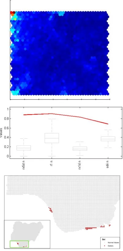
Training was first done using a 20 x 20 hexagonal sheet SOM on all the indices for each year. Outliers were subsequently identified by searching for very high values in a U-matrix. A U-matrix is a visual representation of a self-organizing map (SOM) where the Euclidean distance between neurons are represented in a colour-coded image. If represented as a greyscale image (from white to black), then lighter colours indicate closely spaced neurons while dark colours indicate distant neurons. Therefore, a group of light colours can be regarded as a cluster and the dark colours regarded as boundaries of the cluster. From our analysis, outliers can be clearly identified as bright red spots at the upper left corner of the U-matrix (Figure 4, top graph). Plotting the data on a boxplot confirms them as outliers as they have very large values outside the quantile range of the dataset (Figure 4, middle graph). Further plotting these data (Figure 4, bottom map) shows that they mostly fall in the south eastern and south western region of Nigeria. This region is noted for extremely high precipitation. Hence, it can be argued that these high values are not outliers but simply extreme values which should be of interest for
further analysis. However, including them can significantly impact the overall results. Hence, these outliers were removed to better understand and clustering of the indices values.
Figure 4: U-matrix (top), boxplot (middle) and map (bottom) of the four precipitation indices showing outliers in red in 2003
3.2.2 Spatial trends
A 4 x 1 SOM was used because we wanted to obtain 4 clusters which is in line with number of Koppen climate classification zones over Nigeria. As expected, there is evidence of spatial autocorrelation in the pattern of the clusters (Figure 5). Four regions with similar precipitation characteristics are evident varying from the south to the north through the middle belt of Nigeria. Although these clusters bare some resemblance with the Koppen climatic zones, there are still several variations in the spatial extent of each zone when both are compared. However, this is not surprising since the Koppen classification characterizes mean climatic characteristics, and the clusters are based on extreme precipitation indices. For better clarity in interpretation, we have applied a color scheme to the value of each precipitation index in a tabular form so that we can easily identify the color’s that represent high (red), mean (yellow) and low (green) values of each index. The table in Figure 5 shows the mean value of each index in a cluster.
Cluster 1 covers the Niger-Delta and southeast region of the country. It is characterized by very high precipitation amount, intensity and frequency. This is because of the south-western trade winds that bring a lot of moisture inland from the Atlantic Ocean in the south. Because of the high moisture, this region experiences heavy and abundant monsoonal rainfall and is cloudy all year round. Hence, they have a typical tropical monsoon climate.
Cluster 2 covers the southwest and extends further inland. Although not as high as Cluster 1, it is also characterized by high intensity, frequency and amount of rainfall. This region experiences two peaks of rainfall in a year with a little dry season in August. The first rainfall peak is usually characterized by thunderstorms and occurs in June, while the second rainfall peak is usually monsoonal and occurs around September. A portion of this cluster appears as an island in the middle belt around Jos, Kaduna and Abuja, surrounded by Cluster 3. This might be explained by the terrain of this region, which is a plateau with high elevation. Hence, it has a semi-temperate climate. Therefore, it is interesting to note that it bears similar precipitation characteristics with southwestern Nigeria.
Cluster 3 covers a major part of the middle belt. Unlike Cluster 2, this region exhibits just a single maximum of rainfall during the raining season. Rainfall in this region is primarily associated with thunderstorms and high wind gusts. This is the region where the south-westerlies meet the north-easterlies to create what is known as the Inter Tropical Discontinuity (ITD). The ITD is a region of low pressure and an important factor for Nigeria weather and climate (Odekunle 2010).
Cluster 4 is located predominantly in the northern part of the country. This is a dry and dusty area with the North-Easterly trade winds bringing in dry and dusty air masses from the Sahara Desert. Results show that this region experiences minimal rainfall in terms of amount, duration, frequency and intensity (see table in Figure 5). The raining season in this region is very short lasting just about three months.
Figure 5: Precipitation indices clustering over Nigeria in 2003
3.2.3 Temporal trends
There was a tendency for the maximum 1-day precipitation, maximum 5-day precipitation and frequency of rainy days to increase with time in clusters 1, 2 and 4. In contrast, the maximum 1-day precipitation decreases with time in cluster 3. The intensity of rainfall was constant in cluster 1 throughout the period under study, while a decreasing trend is noticed in rainfall intensity and maximum 1-day precipitation in cluster 3. However, considering the results of the Mann-Kendall test, those trends were not significant (Figure 6). The only statistically significant upward trend is noticed in the frequency of rainy days in cluster 4.
Figure 6:Observed values of the Mann-Kendall’s test statistic ZS
‐2,5 ‐2 ‐1,5 ‐1 ‐0,5 0 0,5 1 1,5 2 2,5 ZS Critical values (=5%)
4
Conclusion
The main objective of this research was to study the spatial and temporal patterns of precipitation extremes in Nigeria. This was achieved by computing a SOM with four precipitation indices computed from 1985 to 2016. The four clusters created for each year summarize the precipitation dynamics that underline the indices. The spatial extents of the clusters have some resemblances with the Koppen climatic zones, but there are some relevant differences throughout the years. We also identified a significant increasing trend in the frequency of rainy days in cluster 4, which predominantly covers the northern part of the country. It is important to note that this trend was measured at the centroid of the cluster, so that conclusion cannot be extrapolated to the whole cluster.
We have been able to identify the spatial and temporal patterns of extreme precipitation, and thus gain valuable insights into the spatial and temporal dynamics of precipitation in Nigeria. However, the temporal resolution of the dataset is too small to adequately characterize the long-term behavior of extreme precipitation in Nigeria. Further research with a higher temporal resolution dataset should be pursued.
Acknowledgements
The work described in this thesis was supported by the European Commission (EC) Education, Audio-visual and Cultural Executive Agency (EACEA) Erasmus Mundus scholarship. The authors also gratefully appreciate the Information Management School of the Universidade Nova de Lisboa (NOVA IMS), department of Geoinformatics at the university of Munster and Universitat Jaume I.
Conflicts of Interest
5 References
Abiodun, Babatunde J., Kamoru A. Lawal, Ayobami T. Salami, and Abayomi A. Abatan. 2013. “Potential Influences of Global Warming on Future Climate and Extreme Events in Nigeria.” Regional Environmental Change 13 (3): 477–91. doi:10.1007/s10113-012-0381-7.
Adejuwon, James O. 2006. “Food Crop Production in Nigeria. II. Potential Effects of Climate Change.” Climate Research 32 (3): 229–45. doi:10.3354/cr032229.
Akinsanola, Akintomide; Ogunjobi Kehinde. 2014. “Analysis of Rainfall and Temperature Variability Over Nigeria.” Global
Journal of Human-Social Science: B Geography, Geo-Sciences, Environmental Disaster Management 14 (3).
Akpodiogaga-, Peter, and Ovuyovwiroye Odjugo. 2009. “Quantifying the Cost of Climate Change Impact in Nigeria: Emphasis on Wind and Rainstorms.” J Hum Ecol 28 (2): 93–101.
Alexander, Lisa V., X. Zhang, T. C. Peterson, J. Caesar, B. Gleason, A. M G Klein Tank, M. Haylock, et al. 2006. “Global Observed Changes in Daily Climate Extremes of Temperature and Precipitation.” Journal of Geophysical Research
Atmospheres 111 (5): 1–22. doi:10.1029/2005JD006290.
Bação, Fernando, and Victor Lobo. 2011. “Fundamentals of Data Preparation and Pre-Processing.”
Bação, Fernando, Victor Lobo, and Marco Painho. 2004. “Geo-Self-Organizing Map (Geo-SOM) for Building and Exploring Homogeneous Regions.” Geographic Information Science. http://link.springer.com/chapter/10.1007/978-3-540-30231-5_2.
Dee, D. P., S. M. Uppala, A. J. Simmons, P. Berrisford, P. Poli, S. Kobayashi, U. Andrae, et al. 2011. “The ERA-Interim Reanalysis: Configuration and Performance of the Data Assimilation System.” Quarterly Journal of the Royal
Meteorological Society 137 (656): 553–97. doi:10.1002/qj.828.
Donat, M. G., L. V. Alexander, H. Yang, I. Durre, R. Vose, R. J H Dunn, K. M. Willett, et al. 2013. “Updated Analyses of Temperature and Precipitation Extreme Indices since the Beginning of the Twentieth Century: The HadEX2 Dataset.”
Journal of Geophysical Research Atmospheres 118 (5): 2098–2118. doi:10.1002/jgrd.50150.
Ekpoh, Imo J, and Ekpenyong Nsa. 2011. “Extreme Climatic Variability in North-Western Nigeria: An Analysis of Rainfall Trends and Patterns.” Journal of Geography and Geology 3 (1): 51–62. doi:10.5539/jgg.v3n1p51.
Enete, Anselm, and Taofeeq Amusa. 2010. “Challenges of Agricultural Adaptation to Climate Change in Nigeria: A Synthesis from the Literature.” Fact Reports 4 (8): 0–8. http://factsreports.revues.org/678.
Funk, C. C., P. J. Peterson, M. F. Landsfeld, D. H. Pedreros, J. P. Verdin, J. D. Rowland, B. E. Romero, G. J. Husak, J. C. Michaelsen, and A. P. Verdin. 2014. “A Quasi-Global Precipitation Time Series for Drought Monitoring.” U.S.
Geological Survey Data Series 832: 4. doi:http://dx.doi.org/110.3133/ds832.
Funk, Chris, Pete Peterson, Martin Landsfeld, Diego Pedreros, James Verdin, Shraddhanand Shukla, Gregory Husak, et al. 2015. “The Climate Hazards Infrared Precipitation with Stations—a New Environmental Record for Monitoring Extremes.”
Scientific Data 2: 150066. doi:10.1038/sdata.2015.66.
Gbode, Imole Ezekiel, Akintomide Afolayan Akinsanola, and Vincent Olanrewaju Ajayi. 2015. “Recent Changes of Some Observed Climate Extreme Events in Kano” 2015.
Gorricha, J., V. Lobo, and A. C. Costa. 2013. “A Framework for Exploratory Analysis of Extreme Weather Events Using Geostatistical Procedures and 3D Self-Organizing Maps.” International Journal on Advances in Intelligent Systems 6 (1&2): 16–26. http://citeseerx.ist.psu.edu/viewdoc/download?doi=10.1.1.360.5951&rep=rep1&type=pdf#page=30. Henriques, Roberto, Fernando Bacao, and Victor Lobo. 2012. “Exploratory Geospatial Data Analysis Using the GeoSOM Suite.”
Computers, Environment and Urban Systems 36 (3). Elsevier Ltd: 218–32. doi:10.1016/j.compenvurbsys.2011.11.003.
Hewitson, B. C., and R. G. Crane. 2005. “Gridded Area-Averaged Daily Precipitation via Conditional Interpolation.” Journal of
Climate 18 (1): 41–57. doi:10.1175/JCLI3246.1.
———. 2006. “Consensus between GCM Climate Change Projections with Empirical Downscaling: Precipitation Downscaling over South Africa.” International Journal of Climatology 26 (10): 1315–37. doi:10.1002/joc.1314.
IPCC. 2007. “Climate Change 2007: The Physical Science Basis. Contribution of Working Group I to the Fourth Assessment Report of the Intergovernmental Panel on Climate Change [Solomon, S., D. Qin, M. Manning, Z. Chen, M. Marquis, K.B. Averyt, M. Tignor and H.L. Miller.” Cambridge University Press, Cambridge, United Kingdom and New York, NY, USA, 1–4. papers3://publication/uuid/789C871F-F7F3-4AD1-A26B-017707E6A214.
———. 2012. Managing the Risks of Extreme Events and Disasters to Advance Climate Change Adaptation. Ipcc. doi:10.1596/978-0-8213-8845-7.
———. 2014. “Climate Change 2014 Synthesis Report.” Contribution of Working Groups I, II and III to the Fifth Assessment
Report of the Intergovernmental Panel on Climate Change, 1–112.
Jones, Mari R., Stephen Blenkinsop, Hayley J. Fowler, and Christopher G. Kilsby. 2014. “Objective Classification of Extreme Rainfall Regions for the UK and Updated Estimates of Trends in Regional Extreme Rainfall.” International Journal of
Climatology 34 (3): 751–65. doi:10.1002/joc.3720.
Jr, William J Gutowski, Francis O Otieno, Raymond W Arritt, and Eugene S Takle. 2004. “Diagnosis and Attribution of a Seasonal Precipitation Deficit in a U . S . Regional Climate Simulation.” Journal of Hydrometeorology 5: 230–42. Karl, Thomas, Neville Nicholls, and Anver Ghazi. 1999. “Workshop on Indices and Indicators for Climate Extremes
Precipitation.pdf.” Climate Change 42: 3–7. doi:10.1007/978-94-015-9265-9_2. Kendal, M.G. 1975. Rank Correlation Methods. Fourth ed. London: Charles Griffin.
Klein Tank, Albert M.G., Francis W Zwiers, and Xuebin Zhang. 2009. “Guidelines on Analysis of Extremes in a Changing Climate in Support of Informed Decisions for Adaptation.” Climate Data and Monitoring, no. WCDMP-No. 72: 52. File Attachment.
Kotsiantis, S B, D Kanellopoulos, and P E Pintelas. 2006. “Data Preprocessing for Supervised Learning.” International Journal
of Computer Science 1 (2): 111–17. doi:10.1080/02331931003692557.
Climate Classification Updated.” Meteorologische Zeitschrift 15 (3): 259–63. doi:10.1127/0941-2948/2006/0130. Mann, H.B. 1945. “Non-Parametric Test Against Trends.” Econometrica 13 (3): 245–59.
Moberg, Anders, Philip D. Jones, David Lister, Alexander Walther, Manola Brunet, Jucundus Jacobeit, Lisa V. Alexander, et al. 2006. “Indices for Daily Temperature and Precipitation Extremes in Europe Analyzed for the Period 1901-2000.” Journal
of Geophysical Research Atmospheres 111 (22). doi:10.1029/2006JD007103.
Obioha, Emeka E. 2008. “Climate Change , Population Drift and Violent Conflict over Land Resources in Northeastern Nigeria.”
Conflict 23 (4): 311–24.
Odekunle, Theophilus. 2010. “An Assessment of the Influence of the Inter-Tropical Discontinuity on Inter-Annual Rainfall Characteristics in Nigeria.” Geographical Research 48 (3): 314–26. doi:10.1111/j.1745-5871.2009.00635.x.
Ogungbenro, Stephen Bunmi, and Tobi Eniolu Morakinyo. 2014. “Rainfall Distribution and Change Detection across Climatic Zones in Nigeria.” Weather and Climate Extremes 5 (1). Elsevier: 1–6. doi:10.1016/j.wace.2014.10.002.
Okoloye, CU, NI Aisiokuebo, JE Ukeje, AC Anuforom, and ID Nnodu. 2013. “RAINFALL VARIABILITY AND THE RECENT CLIMATE EXTREMES IN NIGERIA By.” Journal of Meteorology and Climate Science 11: 49–57.
Olaiya, Folorunsho, and Adesesan Barnabas Adeyemo. 2012. “Application of Data Mining Techniques in Weather Prediction and Climate Change Studies.” International Journal of Information Engineering and Electronic Business 4 (1): 51–59. doi:10.5815/ijieeb.2012.01.07.
Onyekuru, Anthony N, and Rob Marchant. 2014. “Climate Change Impact and Adaptation Pathways for Forest Dependent Livelihood Systems in Nigeria.” African Journal of Agricultural Research 9 (24): 1819–32. doi:10.5897/AJAR2013.8315.
Peterson, T. C. 2005. “Climate Change Indices.” WMO Bulletin 54 (2): 83–86.
Peterson, Thomas C, Christopher Christoper Folland, George Gruza, William Hogg, Abdallah Mokssit, and Neil Plummer. 2001. “Report on the Activities of the Working Group on Climate Change Detection and Related Rapporteurs 1998–2001.” Rep.
WCDMP-47, WMO-TD 1071, no. March: 143. doi:WMO, Rep. WCDMP-47,WMO-TD 1071.
Res, Clim, B C Hewitson, and R G Crane. 2002. “Self-Organizing Maps : Applications to Synoptic Climatology.” Climate
Research 22: 13–26.
Rodrigues, Pedro Marcos Santana. 2010. “An Approach Geo-Data Mining to Climate Regions of the Iberian Peninsula, 1951 - 2010.” New Univerity of Lisbon. https://run.unl.pt/bitstream/10362/18342/1/TSI0111.pdf.
Spanakis, Gerasimos, and Gerhard Weiss. 2016. “AMSOM: Adaptive Moving Self-Organizing Map for Clustering and Visualization.” Proceedings of the 8th International Conference on Agents and Artificial Intelligence, 129–40. doi:10.5220/0005704801290140.
Stefan, Rahmstorf. 2005. “Anthropogenic Climate Change: Revisiting the Facts.” History 140 (6): 34–53. doi:10.1016/j.cell.2010.01.022.
Ta, S, K Y Kouadio, K E Ali, E Toualy, A Aman, and F Yoroba. 2016. “West Africa Extreme Rainfall Events and Large-Scale Ocean Surface and Atmospheric Conditions in the Tropical Atlantic.” Advances in Meteorology 2016: 14. doi:10.1155/2016/1940456.
Thibaud, E., R. Mutzner, and A. C. Davison. 2013. “Threshold Modeling of Extreme Spatial Rainfall.” Water Resources
Research 49 (8): 4633–44. doi:10.1002/wrcr.20329.
Van den Besselaar, E. J M, A. M G Klein Tank, and T. A. Buishand. 2013. “Trends in European Precipitation Extremes over 1951-2010.” International Journal of Climatology 33 (12): 2682–89. doi:10.1002/joc.3619.
Xiaofeng Gong, and M. B. Richman. 1995. “On the Application of Cluster Analysis to Growing Season Precipitation Data in North America East of the Rockies.” Journal of Climate. doi:10.1175/1520-0442(1995)008<0897:OTAOCA>2.0.CO;2.
6 Appendix
Matlab Script
% Clear workspace clear all;
% Specify netcdf filename
filename='D:\CHIRPS DATA\chirps-v2.0.1999.days_p05.nc'; % displaying the structure of the chirps dataset
ncdisp(filename)
% extracting Nigeria from the global chirps dataset based on lon/lat
long = ncread(filename,'longitude')'; % Longitudinal coordinates lat = ncread(filename,'latitude')'; % Latitudinal coordinates
% finding the indices of the latitude within which my grid lies latstart = find(lat>4.0250,1, 'first');
latend = find(lat<14.0250,1, 'last');
% finding the indices of the longitude within which my grid lies lonstart = find(long>2.4750,1, 'first');
lonend = find(long<15,1, 'last');
ncid = netcdf.open(filename,'NOWRITE'); %long= netcdf.getVar(ncid,1); %lat= netcdf.getVar(ncid,0); time= netcdf.getVar(ncid,3); %rr= netcdf.getVar(ncid,2,[latstart,lonstart,1],[(latend-latstart),(lonend-lonstart),355]); %rr= netcdf.getVar(ncid,2,[10,10,10],[10,10,355]); rr= netcdf.getVar(ncid,2,[lonstart,latstart,1],[(lonend-lonstart),(latend-latstart),364]);
[nLong, nLat, nTime]=size(rr);
%[nlong,nlat,ntimes]=size(nigeria1981); longNigeria=long(lonstart:lonend); latNigeria=lat(latstart:latend);
nigeria2015=rr(:,:,:);%:lonend,latstart:latend,366:730); %converting -9999 values to NaN
nigeria2015(nigeria2015 == -9999) = NaN;
rra=zeros(nLong*nLat*nTime,5); counter=1;
for t=1:nTime % for each year ano=floor(t/366)+1;
for la=1:nLat % for each latitude %rra=[rra;
(1:nlong)',ones(nlong,1)*la,ones(nlong,1)*t,ones(nlong,1)*year, nigeria1981(:,la,t)];
rra(counter:counter+nLong-1,1:5)=[(1:nLong)',ones(nLong,1)*la,ones(nLong,1)*t,ones(nLong,1) *2015, nigeria2015(:,la,t)]; counter=counter+nLong; end disp(t); end rra=sortrows(rra,[1,2]); rrSoma5=zeros(size(rra,1),2);
for ano=2015:2015 % for the year under consideration indAno=find(rra(:,4)==ano); %indices do ano
for i=1:size(indAno,1)-4 % para cada dia de um ano valor=rra(indAno(i):indAno(i)+4,5);
rrSoma5(indAno(i),1)=sum(valor(valor>=1)); %long lat dia ano rr
rrSoma5(indAno(i),2)=rra(indAno(i),4); end
end
%max por ano do rrSOMA R5X=zeros(nLat*nLong,5); counter=1;
for ano=2015:2015 % for the year under consideration for lo=1:nLong
for la=1:nLat
indAno=find(rra(:,1)==lo & rra(:,2)==la & rra(:,4)==ano); %indices de uma long uma lat e um ano [M, I]=max(rrSoma5(indAno,1)); %R5X=[R5X; lo,la,ano,I,M]; R5X(counter,:)=[lo,la,ano,I,M]; counter=counter+1; disp(counter); end end disp(ano) end %calculating r1 R1=zeros(nLong*nLat,3); counter=1; for lo=1:nLong for la=1:nLat R1(counter,:)=[lo,la,size(find(nigeria2015(lo,la,:)>1),1)]; counter=counter+1; end end %calculating rx1d Rx1d=zeros(nLong*nLat,3); counter=1; for lo=1:nLong for la=1:nLat
Rx1d(counter,:)=[lo,la,max(nigeria2015(lo,la,:))]; counter=counter+1; end end %calculating sdii SDII=zeros(nLong*nLat,3); counter=1; %sumPrecBig1=sum(rr>1,3); for lo=1:nLong for la=1:nLat SDII(counter,:)=[lo,la,sum(nigeria2015(lo,la,nigeria2015(lo,la,:) >1))./size(find(nigeria2015(lo,la,:)>1),1)]; %SDII(counter,:)=[lo,la,((sum(rr>1,3)./(size(find(rr>1),1))))]; counter=counter+1; end end
%arranging all calculated values into columns
R5XD=[longNigeria(R5X(:,1))',latNigeria(R5X(:,2))',R5X(:,3),R5X(: ,5),R1(:,3), Rx1d(:,3), SDII(:,3)];
%R1=[longNigeria(R1(:,1)),latNigeria(R1(:,2))',R5X(:,5)]; %need to perfect export to csv/text
Descriptive Statistics
1985 rx5d r1 rx1d sdii Mean 92.51 113.14 43.67 9.84 Standard Error 0.18 0.24 0.07 0.01 Median 87.43 111.00 41.66 9.73 Mode 110.89 96.00 62.79 12.64 Standard Deviation 30.54 41.95 12.67 1.96 Sample Variance 932.42 1760.00 160.59 3.83 Kurtosis 2.63 -0.12 2.78 1.78 Skewness 1.28 0.51 1.11 0.74 Range 260.63 205.00 129.03 17.18 Minimum 24.29 36.00 12.69 4.38 Maximum 284.92 241.00 141.72 21.56 Sum 2789599.82 3411723.00 1316824.45 296735.27 Count 30155.00 30155.00 30155.00 30155.00 1986 rx5d r1 rx1d sdii Mean 93.12 98.07 46.62 10.80 Standard Error 0.20 0.19 0.11 0.01 Median 86.00 96.00 41.81 10.55 Mode 136.65 95.00 79.64 14.03 Standard Deviation 35.48 32.98 19.81 2.08 Sample Variance 1258.74 1087.54 392.40 4.32 Kurtosis 6.95 0.11 11.12 1.49 Skewness 2.05 0.53 2.40 0.77 Range 335.98 178.00 224.45 17.77 Minimum 25.80 29.00 15.16 4.88 Maximum 361.79 207.00 239.61 22.64 Sum 2808139.40 2957151.00 1405906.95 325731.75 Count 30155.00 30155.00 30155.00 30155.00 1987 rx5d r1 rx1d sdii Mean 90.98 102.49 43.25 9.79 Standard Error 0.22 0.24 0.10 0.01 Median 86.83 99.00 41.67 9.57 Mode 115.42 85.00 73.27 12.20 Standard Deviation 37.88 40.81 16.90 2.33 Sample Variance 1435.09 1665.50 285.63 5.45 Kurtosis 2.97 -0.56 0.87 1.12 Skewness 1.30 0.38 0.76 0.70 Range 315.05 202.00 153.26 19.10 Minimum 23.92 23.00 10.84 3.67 Maximum 338.97 225.00 164.10 22.77 Sum 2743526.14 3090601.00 1304068.45 295317.59 Count 30155.00 30155.00 30155.00 30155.001988 rx5d r1 rx1d sdii Mean 100.80 113.55 44.49 10.24 Standard Error 0.18 0.22 0.07 0.01 Median 94.29 108.00 42.51 10.15 Mode 133.48 103.00 71.85 13.17 Standard Deviation 30.42 38.34 11.60 1.62 Sample Variance 925.51 1469.74 134.51 2.63 Kurtosis 1.94 0.69 1.78 1.80 Skewness 1.22 0.91 0.96 0.56 Range 243.26 200.00 111.57 16.54 Minimum 34.41 42.00 15.18 4.13 Maximum 277.67 242.00 126.75 20.67 Sum 3039499.66 3424143.00 1341574.74 308639.68 Count 30155.00 30155.00 30155.00 30155.00 1989 rx5d r1 rx1d sdii Mean 96.17 109.80 45.16 10.60 Standard Error 0.18 0.21 0.10 0.01 Median 91.88 107.00 41.61 10.25 Mode 92.60 95.00 82.90 14.07 Standard Deviation 31.66 36.22 16.63 2.19 Sample Variance 1002.13 1312.20 276.66 4.79 Kurtosis 1.51 -0.29 2.04 0.47 Skewness 0.97 0.38 1.26 0.45 Range 270.82 182.00 128.41 17.54 Minimum 19.15 31.00 8.96 3.36 Maximum 289.97 213.00 137.37 20.89 Sum 2899955.10 3311083.00 1361899.24 319585.62 Count 30155.00 30155.00 30155.00 30155.00 1990 rx5d r1 rx1d sdii Mean 91.82 106.00 40.14 10.40 Standard Error 0.29 0.22 0.11 0.02 Median 78.62 104.00 35.44 9.71 Mode 80.99 105.00 71.94 14.08 Standard Deviation 50.29 38.33 18.63 2.74 Sample Variance 2529.51 1469.08 346.92 7.51 Kurtosis 9.02 -0.21 9.01 1.07 Skewness 2.73 0.42 2.55 0.98 Range 449.58 196.00 185.68 21.22 Minimum 19.80 26.00 10.14 3.79 Maximum 469.38 222.00 195.81 25.00 Sum 2768857.96 3196501.00 1210395.90 313630.13 Count 30155.00 30155.00 30155.00 30155.00
1991 rx5d r1 rx1d sdii Mean 101.36 111.44 46.38 10.87 Standard Error 0.22 0.20 0.10 0.01 Median 92.10 112.00 42.13 10.41 Mode 157.12 115.00 92.02 18.43 Standard Deviation 37.45 34.08 16.88 2.55 Sample Variance 1402.75 1161.51 284.84 6.53 Kurtosis 4.19 -0.32 4.70 2.94 Skewness 1.73 0.25 1.68 1.37 Range 353.44 178.00 195.59 21.38 Minimum 33.60 37.00 15.52 4.72 Maximum 387.03 215.00 211.11 26.10 Sum 3056414.50 3360475.00 1398446.83 327715.26 Count 30155.00 30155.00 30155.00 30155.00 1992 rx5d r1 rx1d sdii Mean 97.27 102.94 44.75 10.77 Standard Error 0.20 0.18 0.09 0.01 Median 92.12 101.00 41.70 10.47 Mode 132.94 99.00 68.50 13.46 Standard Deviation 34.94 31.17 15.81 2.39 Sample Variance 1220.76 971.58 250.04 5.71 Kurtosis 6.97 -0.08 4.44 4.99 Skewness 1.87 0.36 1.52 1.52 Range 347.18 173.00 149.38 23.93 Minimum 19.47 33.00 9.34 4.12 Maximum 366.65 206.00 158.72 28.05 Sum 2933321.98 3104173.00 1349451.72 324657.00 Count 30155.00 30155.00 30155.00 30155.00 1993 rx5d r1 rx1d sdii Mean 95.49 111.72 48.56 10.17 Standard Error 0.20 0.23 0.10 0.01 Median 88.50 108.00 45.27 9.86 Mode 164.15 98.00 49.37 13.43 Standard Deviation 33.90 40.15 17.83 2.14 Sample Variance 1149.54 1612.16 317.87 4.56 Kurtosis 6.59 -0.16 6.49 1.17 Skewness 1.96 0.49 1.81 0.75 Range 391.55 212.00 237.55 18.91 Minimum 23.40 30.00 9.92 4.13 Maximum 414.94 242.00 247.46 23.04 Sum 2879528.84 3368913.00 1464215.87 306682.61 Count 30155.00 30155.00 30155.00 30155.00
1994 rx5d r1 rx1d sdii Mean 104.10 110.32 46.91 11.19 Standard Error 0.17 0.18 0.10 0.01 Median 99.15 110.00 42.97 10.71 Mode 100.91 103.00 49.26 10.10 Standard Deviation 29.37 31.74 16.83 2.43 Sample Variance 862.60 1007.70 283.38 5.91 Kurtosis 7.97 -0.07 7.28 5.60 Skewness 2.11 0.22 2.21 1.86 Range 356.80 174.00 158.27 23.45 Minimum 42.16 36.00 19.00 5.08 Maximum 398.96 210.00 177.27 28.52 Sum 3139186.67 3326700.00 1414535.20 337326.00 Count 30155.00 30155.00 30155.00 30155.00 1995 rx5d r1 rx1d sdii Mean 94.08 113.45 44.26 10.85 Standard Error 0.21 0.22 0.10 0.02 Median 85.91 113.00 40.24 10.26 Mode 117.35 115.00 47.50 16.45 Standard Deviation 36.62 37.93 17.82 2.77 Sample Variance 1341.21 1438.43 317.58 7.65 Kurtosis 7.52 -0.44 4.68 2.44 Skewness 2.33 0.29 1.85 1.32 Range 336.97 194.00 156.07 21.98 Minimum 24.56 34.00 11.63 4.46 Maximum 361.53 228.00 167.69 26.43 Sum 2837048.01 3421046.00 1334767.78 327190.14 Count 30155.00 30155.00 30155.00 30155.00 1996 rx5d r1 rx1d sdii Mean 99.14 104.88 43.62 11.45 Standard Error 0.23 0.18 0.09 0.02 Median 91.96 103.00 41.09 11.07 Mode 132.93 108.00 64.75 16.89 Standard Deviation 39.13 30.48 14.91 2.93 Sample Variance 1531.34 929.00 222.26 8.60 Kurtosis 4.63 0.52 4.26 1.58 Skewness 1.75 0.62 1.54 0.76 Range 309.28 187.00 137.45 23.67 Minimum 22.57 33.00 9.45 3.91 Maximum 331.85 220.00 146.90 27.58 Sum 2989632.07 3162547.00 1315308.19 345281.58 Count 30155.00 30155.00 30155.00 30155.00
1997 rx5d r1 rx1d sdii Mean 90.35 119.12 43.10 10.02 Standard Error 0.20 0.20 0.10 0.01 Median 83.49 119.00 38.65 9.55 Mode 104.65 119.00 60.34 14.14 Standard Deviation 35.52 35.58 17.73 2.60 Sample Variance 1261.97 1265.64 314.34 6.74 Kurtosis 5.79 0.05 13.71 2.31 Skewness 1.96 0.21 2.89 1.20 Range 333.53 200.00 227.99 21.72 Minimum 28.23 33.00 14.16 4.39 Maximum 361.76 233.00 242.15 26.10 Sum 2724358.04 3592121.00 1299671.29 302274.29 Count 30155.00 30155.00 30155.00 30155.00 1998 rx5d r1 rx1d sdii Mean 94.35 105.08 43.22 11.35 Standard Error 0.18 0.18 0.07 0.01 Median 87.24 102.00 40.84 10.95 Mode 94.68 98.00 46.94 14.86 Standard Deviation 30.91 30.69 13.01 2.19 Sample Variance 955.63 941.82 169.29 4.81 Kurtosis 8.32 0.98 3.26 2.65 Skewness 2.39 0.68 1.37 1.15 Range 276.96 175.00 127.57 22.24 Minimum 34.08 36.00 13.59 4.64 Maximum 311.04 211.00 141.16 26.88 Sum 2845069.83 3168827.00 1303425.93 342258.19 Count 30155.00 30155.00 30155.00 30155.00 1999 rx5d r1 rx1d sdii Mean 102.47 114.68 44.06 11.61 Standard Error 0.20 0.22 0.09 0.01 Median 94.41 113.00 40.38 11.09 Mode 147.53 112.00 72.13 14.55 Standard Deviation 35.43 37.55 15.79 2.26 Sample Variance 1255.10 1410.37 249.43 5.09 Kurtosis 6.50 -0.10 3.71 3.41 Skewness 2.04 0.40 1.63 1.40 Range 288.71 200.00 127.40 24.31 Minimum 37.27 39.00 16.76 4.80 Maximum 325.98 239.00 144.15 29.11 Sum 3089952.86 3458134.00 1328546.62 350210.70 Count 30155.00 30155.00 30155.00 30155.00
2000 rx5d r1 rx1d sdii Mean 92.68 104.30 43.28 10.89 Standard Error 0.18 0.21 0.10 0.01 Median 85.94 102.00 39.00 10.55 Mode 154.05 103.00 39.96 17.24 Standard Deviation 32.08 35.73 17.05 2.23 Sample Variance 1028.82 1276.29 290.55 4.97 Kurtosis 4.35 0.05 6.18 2.11 Skewness 1.73 0.55 2.09 0.77 Range 265.60 193.00 160.71 21.40 Minimum 23.41 29.00 9.55 3.96 Maximum 289.01 222.00 170.26 25.36 Sum 2794846.39 3145117.00 1305216.73 328299.49 Count 30155.00 30155.00 30155.00 30155.00 2001 rx5d r1 rx1d sdii Mean 86.01 102.17 41.04 10.37 Standard Error 0.16 0.15 0.08 0.01 Median 81.71 99.00 38.40 10.23 Mode 110.60 96.00 45.82 9.24 Standard Deviation 27.40 26.77 14.75 2.18 Sample Variance 750.71 716.57 217.46 4.74 Kurtosis 2.32 0.34 4.43 1.27 Skewness 1.05 0.54 1.50 0.51 Range 253.29 177.00 143.18 19.29 Minimum 24.90 31.00 10.54 3.58 Maximum 278.19 208.00 153.72 22.87 Sum 2593541.79 3080978.00 1237474.21 312839.22 Count 30155.00 30155.00 30155.00 30155.00 2002 rx5d r1 rx1d sdii Mean 88.00 111.83 41.56 10.48 Standard Error 0.20 0.20 0.11 0.01 Median 81.55 112.00 37.10 9.89 Mode 110.99 116.00 64.89 14.74 Standard Deviation 34.00 34.75 18.31 2.49 Sample Variance 1156.05 1207.54 335.11 6.22 Kurtosis 7.86 -0.11 11.47 3.97 Skewness 2.21 0.24 2.64 1.46 Range 339.03 186.00 186.11 24.69 Minimum 19.62 29.00 11.45 3.55 Maximum 358.65 215.00 197.57 28.24 Sum 2653572.21 3372224.00 1253124.45 316107.37 Count 30155.00 30155.00 30155.00 30155.00
2003 rx5d r1 rx1d sdii Mean 92.11 109.04 40.75 10.91 Standard Error 0.16 0.20 0.08 0.01 Median 87.43 106.00 37.34 10.63 Mode 143.15 105.00 71.64 14.21 Standard Deviation 27.81 34.79 13.50 1.64 Sample Variance 773.22 1210.32 182.17 2.68 Kurtosis 3.17 0.09 6.74 3.24 Skewness 1.15 0.51 2.03 1.08 Range 335.03 192.00 176.69 19.61 Minimum 29.78 33.00 10.14 3.49 Maximum 364.81 225.00 186.82 23.10 Sum 2777697.74 3288139.00 1228725.35 328950.28 Count 30155.00 30155.00 30155.00 30155.00 2004 rx5d r1 rx1d sdii Mean 92.88 107.95 42.13 10.44 Standard Error 0.18 0.19 0.10 0.01 Median 84.56 107.00 37.37 10.18 Mode 87.05 109.00 80.64 14.05 Standard Deviation 31.91 32.96 16.59 2.40 Sample Variance 1018.33 1086.59 275.07 5.78 Kurtosis 5.40 -0.18 8.28 2.15 Skewness 1.91 0.25 2.19 0.94 Range 374.08 184.00 259.71 21.96 Minimum 30.12 23.00 11.46 4.36 Maximum 404.20 207.00 271.16 26.32 Sum 2800663.39 3255092.00 1270506.54 314926.78 Count 30155.00 30155.00 30155.00 30155.00 2005 rx5d r1 rx1d sdii Mean 94.78 104.10 46.86 10.63 Standard Error 0.21 0.18 0.13 0.01 Median 86.39 103.00 40.99 10.23 Mode 156.39 105.00 122.93 14.38 Standard Deviation 36.27 31.57 21.82 2.15 Sample Variance 1315.61 996.94 476.21 4.64 Kurtosis 3.98 0.17 6.86 2.15 Skewness 1.78 0.56 2.43 1.08 Range 290.87 186.00 178.48 19.59 Minimum 23.97 36.00 13.48 4.29 Maximum 314.84 222.00 191.95 23.89 Sum 2858217.64 3139031.00 1413061.56 320577.26 Count 30155.00 30155.00 30155.00 30155.00
2006 rx5d r1 rx1d sdii Mean 112.25 113.67 47.56 10.92 Standard Error 0.29 0.21 0.12 0.01 Median 97.30 110.00 41.84 10.55 Mode 165.83 105.00 52.11 14.05 Standard Deviation 50.20 35.74 20.91 2.31 Sample Variance 2519.87 1277.70 437.42 5.34 Kurtosis 6.56 0.27 8.55 2.25 Skewness 2.25 0.55 2.52 1.07 Range 477.08 213.00 212.29 20.70 Minimum 24.88 28.00 15.99 4.75 Maximum 501.97 241.00 228.28 25.45 Sum 3384817.04 3427764.00 1434173.18 329331.68 Count 30155.00 30155.00 30155.00 30155.00 2007 rx5d r1 rx1d sdii Mean 103.33 110.86 47.88 10.74 Standard Error 0.25 0.21 0.12 0.01 Median 90.40 110.00 42.17 10.22 Mode 212.03 109.00 76.80 13.33 Standard Deviation 42.98 36.44 20.40 2.33 Sample Variance 1847.00 1328.07 416.13 5.44 Kurtosis 5.05 -0.08 7.22 2.01 Skewness 1.96 0.35 2.31 1.18 Range 369.51 194.00 231.81 21.50 Minimum 37.22 32.00 15.65 4.36 Maximum 406.73 226.00 247.46 25.86 Sum 3115899.92 3343044.00 1443942.29 323880.33 Count 30155.00 30155.00 30155.00 30155.00 2008 rx5d r1 rx1d sdii Mean 100.41 112.20 44.27 10.78 Standard Error 0.15 0.21 0.09 0.01 Median 97.85 109.00 40.81 10.64 Mode 149.41 109.00 58.61 14.47 Standard Deviation 26.51 36.46 15.76 2.17 Sample Variance 703.01 1329.31 248.53 4.72 Kurtosis 1.77 -0.01 3.29 1.77 Skewness 0.74 0.49 1.50 0.61 Range 254.61 194.00 160.52 20.06 Minimum 23.18 34.00 9.83 3.94 Maximum 277.78 228.00 170.35 24.00 Sum 3027761.07 3383506.00 1334993.91 325174.11 Count 30155.00 30155.00 30155.00 30155.00
2009 rx5d r1 rx1d sdii Mean 97.59 114.28 45.39 10.27 Standard Error 0.27 0.22 0.14 0.02 Median 88.11 113.00 39.13 9.94 Mode 163.39 116.00 144.22 17.34 Standard Deviation 47.65 37.56 24.84 3.05 Sample Variance 2270.18 1410.76 616.80 9.28 Kurtosis 4.76 -0.23 6.27 1.88 Skewness 1.86 0.37 2.25 1.02 Range 365.63 203.00 213.01 23.16 Minimum 21.28 31.00 8.09 3.69 Maximum 386.91 234.00 221.10 26.85 Sum 2942807.95 3446101.00 1368587.38 309801.73 Count 30155.00 30155.00 30155.00 30155.00 2010 rx5d r1 rx1d sdii Mean 100.82 114.84 46.09 10.64 Standard Error 0.18 0.19 0.10 0.01 Median 95.07 112.00 42.09 10.25 Mode 141.64 107.00 55.73 13.41 Standard Deviation 30.98 33.68 17.34 2.33 Sample Variance 959.83 1134.38 300.84 5.43 Kurtosis 4.44 -0.04 1.20 1.76 Skewness 1.45 0.35 1.06 0.95 Range 357.25 191.00 140.77 20.31 Minimum 24.37 35.00 10.59 3.95 Maximum 381.62 226.00 151.36 24.26 Sum 3040108.71 3463043.00 1389907.36 320855.45 Count 30155.00 30155.00 30155.00 30155.00 2011 rx5d r1 rx1d sdii Mean 95.54 113.01 44.13 10.15 Standard Error 0.19 0.21 0.10 0.01 Median 89.45 110.00 41.16 9.71 Mode 102.71 107.00 44.47 14.58 Standard Deviation 32.95 36.78 16.66 2.35 Sample Variance 1085.98 1352.47 277.61 5.53 Kurtosis 4.63 0.06 6.76 2.74 Skewness 1.73 0.53 2.01 1.29 Range 272.98 196.00 153.00 19.82 Minimum 33.82 36.00 12.35 4.31 Maximum 306.80 232.00 165.35 24.12 Sum 2881138.01 3407778.00 1330777.51 306026.34 Count 30155.00 30155.00 30155.00 30155.00
2012 rx5d r1 rx1d sdii Mean 95.79 114.93 45.84 10.90 Standard Error 0.18 0.20 0.09 0.01 Median 86.47 113.00 41.68 10.43 Mode 160.14 106.00 73.25 13.40 Standard Deviation 31.75 34.43 16.07 2.01 Sample Variance 1007.89 1185.50 258.35 4.05 Kurtosis 3.50 -0.08 3.38 2.18 Skewness 1.67 0.35 1.64 1.17 Range 286.86 181.00 132.61 18.99 Minimum 39.50 42.00 17.43 4.44 Maximum 326.36 223.00 150.05 23.43 Sum 2888443.92 3465668.00 1382283.62 328704.07 Count 30155.00 30155.00 30155.00 30155.00 2013 rx5d r1 rx1d sdii Mean 85.89 115.69 43.26 8.70 Standard Error 0.18 0.23 0.09 0.01 Median 79.46 111.00 39.94 8.40 Mode 111.16 105.00 70.39 11.43 Standard Deviation 30.64 39.38 15.12 1.70 Sample Variance 938.62 1551.06 228.61 2.91 Kurtosis 10.81 0.05 2.63 3.19 Skewness 2.58 0.60 1.28 1.24 Range 301.85 211.00 158.45 16.74 Minimum 28.78 33.00 13.48 3.73 Maximum 330.63 244.00 171.93 20.47 Sum 2590070.87 3488513.00 1304481.69 262239.81 Count 30155.00 30155.00 30155.00 30155.00 2014 rx5d r1 rx1d sdii Mean 91.58 113.14 42.46 9.73 Standard Error 0.17 0.20 0.09 0.01 Median 83.50 113.00 39.21 9.45 Mode 136.66 113.00 48.83 14.09 Standard Deviation 30.28 35.37 14.94 2.00 Sample Variance 916.83 1250.73 223.16 4.02 Kurtosis 4.28 -0.27 4.96 1.38 Skewness 1.88 0.08 1.76 0.83 Range 246.03 184.00 158.45 18.07 Minimum 32.16 28.00 13.67 3.98 Maximum 278.19 212.00 172.11 22.05 Sum 2761725.31 3411769.00 1280476.72 293387.46 Count 30155.00 30155.00 30155.00 30155.00
2015 rx5d r1 rx1d sdii Mean 103.61 99.02 44.34 10.86 Standard Error 0.21 0.17 0.10 0.01 Median 93.33 97.00 39.39 10.44 Mode 93.04 97.00 64.57 13.92 Standard Deviation 36.37 29.41 16.91 1.98 Sample Variance 1322.86 864.86 285.89 3.91 Kurtosis 0.55 0.56 3.36 0.92 Skewness 1.00 0.59 1.63 0.90 Range 241.12 187.00 166.88 17.98 Minimum 30.58 27.00 14.18 3.98 Maximum 271.70 214.00 181.06 21.96 Sum 3124235.25 2985800.00 1337129.57 327412.46 Count 30155.00 30155.00 30155.00 30155.00
Histograms
1985 0 1000 2000 3000 4000 5000 6000 20 40 60 80 100 120 140 160 018 200 220 240 260 280 300 Bin RX5D 0 500 1000 1500 2000 2500 3000 3500 Bin R1 0 2000 4000 6000 8000 10000 12000 20 30 40 50 60 70 80 90 100 110 120 130 140 150 Mo re Bin RX1D 0 1000 2000 3000 4000 5000 6000 7000 8000 Bin SDII1986 1987 0 1000 2000 3000 4000 5000 6000 20 40 60 80 100 120 140 160 180 200 220 240 260 280 300 320 340 360 Mo re Bin RX5D 0 500 1000 1500 2000 2500 3000 3500 4000 4500 20 50 80 110 140 170 200 Bin R1 0 1000 2000 3000 4000 5000 6000 7000 8000 9000 10000 20 50 80 110 140 170 200 230 Bin RX1D 0 1000 2000 3000 4000 5000 6000 7000 8000 1 4 7 10 13 16 19 22 Bin SDII 0 500 1000 1500 2000 2500 3000 3500 4000 20 40 60 80 100 120 140 160 180 020 220 240 260 280 300 320 340 Bin RX5D 0 500 1000 1500 2000 2500 3000 3500 Bin R1 0 1000 2000 3000 4000 5000 6000 7000 8000 20 30 40 50 60 70 80 90 100 110 120 130 140 150 160 170 Mo re Bin RX1D 0 1000 2000 3000 4000 5000 6000 7000 Bin SDII
1988 1989 0 1000 2000 3000 4000 5000 6000 Bin RX5D 0 500 1000 1500 2000 2500 3000 3500 4000 4500 20 50 80 110 140 170 200 230 More Bin R1 0 2000 4000 6000 8000 10000 12000 20 40 60 80 100 120 More Bin RX1D 0 1000 2000 3000 4000 5000 6000 7000 8000 9000 1 4 7 10 13 16 19 Bin SDII 0 1000 2000 3000 4000 5000 6000 Bin RX5D 0 500 1000 1500 2000 2500 3000 3500 4000 20 50 80 110 140 170 200 230 Bin R1 0 1000 2000 3000 4000 5000 6000 7000 8000 9000 10000 20 40 60 80 100 120 140 Bin RX1D 0 1000 2000 3000 4000 5000 6000 7000 8000 1 4 7 10 13 16 19 Bin SDII
1990 1991 0 1000 2000 3000 4000 5000 6000 7000 20 50 80 110 140 170 200 230 026 290 320 350 380 410 440 470 Bin RX5D 0 500 1000 1500 2000 2500 3000 3500 4000 20 50 80 110 140 170 200 230 Bin R1 0 2000 4000 6000 8000 10000 12000 14000 20 40 60 80 100 120 140 160 180 200 Bin RX1D 0 1000 2000 3000 4000 5000 6000 7000 1 4 7 10 13 16 19 22 25 Bin SDII 0 1000 2000 3000 4000 5000 6000 20 40 60 80 100 120 140 160 180 200 022 240 260 280 030 320 340 360 380 Mo re Bin RX5D 0 500 1000 1500 2000 2500 3000 3500 4000 4500 20 50 80 110 140 170 200 More Bin R1 0 2000 4000 6000 8000 10000 12000 20 50 80 110 140 170 200 More Bin RX1D 0 1000 2000 3000 4000 5000 6000 7000 8000 Bin SDII
1992 1993 0 500 1000 1500 2000 2500 3000 3500 4000 4500 5000 20 40 60 80 100 120 140 160 180 200 220 240 260 280 300 320 340 360 Mo re Bin RX5D 0 500 1000 1500 2000 2500 3000 3500 4000 4500 20 50 80 110 140 170 200 Bin R1 0 2000 4000 6000 8000 10000 12000 20 40 60 80 100 120 140 160 Bin RX1D 0 1000 2000 3000 4000 5000 6000 7000 8000 9000 Bin SDII 0 1000 2000 3000 4000 5000 6000 20 50 80 110 140 170 200 023 260 290 320 350 380 410 Bin RX5D 0 500 1000 1500 2000 2500 3000 3500 4000 20 50 80 110 140 170 200 230 More Bin R1 0 1000 2000 3000 4000 5000 6000 7000 8000 9000 10000 20 50 80 110 140 170 200 230 More Bin RX1D 0 1000 2000 3000 4000 5000 6000 7000 8000 1 4 7 10 13 16 19 22 More Bin SDII
1994 1995 0 1000 2000 3000 4000 5000 6000 7000 20 40 60 80 100 120 014 160 180 200 220 240 260 280 300 032 340 360 380 400 Bin RX5D 0 1000 2000 3000 4000 5000 6000 Bin R1 0 2000 4000 6000 8000 10000 12000 20 30 40 50 60 70 80 90 100 110 012 130 140 150 160 170 180 Mo re Bin RX1D 0 1000 2000 3000 4000 5000 6000 7000 1 3 5 7 9 11 13 15 17 19 21 23 25 27 29 Bin SDII 0 1000 2000 3000 4000 5000 6000 7000 20 40 60 80 100 120 140 160 180 200 220 240 260 280 300 320 340 360 Mo re Bin RX5D 0 500 1000 1500 2000 2500 3000 3500 4000 20 50 80 110 140 170 200 230 Bin R1 0 2000 4000 6000 8000 10000 12000 20 40 60 80 100 120 140 160 More Bin RX1D 0 1000 2000 3000 4000 5000 6000 7000 Bin SDII
1996 1997 0 1000 2000 3000 4000 5000 6000 Bin RX5D 0 500 1000 1500 2000 2500 3000 3500 4000 4500 5000 20 50 80 110 140 170 200 More Bin R1 0 2000 4000 6000 8000 10000 12000 20 40 60 80 100 120 140 More Bin RX1D 0 1000 2000 3000 4000 5000 6000 7000 Bin SDII 0 1000 2000 3000 4000 5000 6000 20 40 60 80 100 120 140 160 180 200 220 240 260 280 300 320 340 360 Mo re Bin RX5D 0 500 1000 1500 2000 2500 3000 3500 4000 4500 20 50 80 110 140 170 200 230 Bin R1 0 2000 4000 6000 8000 10000 12000 14000 20 50 80 110 140 170 200 230 More Bin RX1D 0 1000 2000 3000 4000 5000 6000 7000 Bin SDII