eve asholanda Global Analysis of Laminated Tubes

GLOBAL ANALYSIS OF LAMINATED TUBES

Luiz A. T. Mororóa, Antônio M. C. Meloa, Evandro Parente Jr.a, Áurea S. Holandab and Daniel C. Almeidaa

a

Departamento de Engenharia Estrutural e Construção Civil, Universidade Federal do Ceará, Campus do Pici, Bloco 710, 60455-760, Fortaleza, Ceará, Brasil, luizmororo@hotmail.com,

macario@ufc.br, evandro@ufc.br, dalmeidaniel@gmail.com

b

Departamento de Engenharia de Transportes, Universidade Federal do Ceará, Campus do Pici, Bloco 703, 60455-760, Fortaleza, Ceará, Brasil, aurea@det.ufc.br

Keywords: Laminated Tubes, Composite Materials, Global-Local Analysis.

Abstract. The finite element analysis of homogenous and isotropic tubes is a well established subject and very good results are obtained for long tubes using standard beam elements. On the other hand, the analysis of laminated composite tubes is generally carried-out using a global-local approach. This approach is performed in two levels, by means of a global analysis using beam elements with effective stiffness properties followed by the analysis of a refined local model of shell or solid elements to compute the ply stresses at critical sections of the tube. This work investigates the use of a global approach to carry-out the complete structural analysis of laminated composite beams, without the need to use a local finite element model. The successful application of beam elements depends on the accurate evaluation of effective mechanical properties of laminated tubes. In this work, the axial and bending stiffness of laminated tubes are computed by appropriate integration of segment stiffness over the tube cross-section. The internal forces obtained from the global analysis are used to compute the beam membrane strain and curvature. Ply strains are computed from the laminated strains. Finally, the stresses in the material system are evaluated using the appropriate constitutive relations. Numerical examples are presented and the results obtained by the global analysis approach are compared with results obtained by solid and shell finite elements. Very good results were obtained for most lamination schemes.

1 INTRODUCTION

Many applications in structural design involve situations where a more detailed response of a small region of a large structure is required by the designer. In such cases, it is needed to construct a mesh, fine enough to capture stress and strains states at the local region of interest (Voleti et al., 1994). Usually, this approach results in a mesh with an excessive number of degrees of freedom leading to a high computational cost. For laminated composite tubes, the use of shell or solid elements is natural, since they allow the precise representation of the adopted tube lay-up as well as the evaluation of stresses and strains in each ply.

For long composite tubes, as marine risers and pipelines, the computational cost of using shell or solid finite element models is prohibitive. Therefore, a practical alternative is to use a global-local approach. Global-local analysis refers to a methodology where the structure is evaluated in two levels. At the global level, the structure is analyzed using a simplified finite element model (e.g. a coarse finite element mesh or a beam element model). After that, the region of interest is analyzed using a refined finite element model with relevant data obtained from global analysis. For tubular structures, the global analysis is carried-out using two and three-dimensional beam elements yielding the global displacements, rotations, and internal forces (axial force, bending and torsional moments). After that, critical locations along the length of the tube are selected and analyzed using a refined model discretized using shell or solid elements subjected to the displacements and/or internal forces computed in the global analysis. The use of beam elements allows the consideration of dynamic and large displacement effects in a simple and efficient way. Furthermore, the global-local approach allows the use trusted finite element programs for analysis of marine risers and pipelines.

The global-local approach is much more computationally efficient than the use of a refined global model. However, it requires the handling of two different finite element models and the transference of the global responses to the local model, which is cumbersome and error prone.

In this work, a simpler approach to the structural analysis of long tubes, as marine risers and pipelines, will be presented. In this approach, the whole structural analysis will be carried-out using a global (beam) model, including the evaluation of stresses and strains in each composite ply.

material system are evaluated using the appropriate constitutive relations.

This paper is organized as follows. Section 2 discusses the computation of the equivalent mechanical properties of laminated composite tubes. Section 3 presents the procedure for computation of ply stresses and strains. Section 4 presents the numerical examples. Finally, Section 5 presents the main conclusions.

2 EQUIVALENT MECHANICAL PROPERTIES OF LAMINATED TUBES

Laminated tubes are formed by a set of layers stacked to achieve the desired stiffness and thickness, as depicted in Figure 1. The global x-axis is parallel to the longitudinal direction of the tube, while the global axis y and z are parallel to the tube cross-section. The effective mechanical properties will be computed in the global axes.

Figure 1: Laminated tube.

In addition to the global axes, two set of local axes will be used: the segment and the material (or ply) system. The segment (or laminate) system (x, r, s), depicted in

Figure 2, will be used in the computation of the laminate stiffness. It can be noted that r is the radial direction and s is tangent to the laminate mid-surface (hoop direction). Finally, the material system (x1, x2, x3), where 1 is the fiber direction, 2 is the in-plane transversal direction and 3 is the out-of-plane (i.e. radial) direction, will be used to define the stress-deformation relations for each lamina.

s s s b

e q

e z

y r

r r

R



y z

x

z

y

Macroscopically, each lamina behaves as a homogenous and orthotropic material. Assuming a plane stress state in each ply, the relation between stress (1) and strain

(1) in the material system is given by generalizes Hooke’s law:

1 1 6 2 1 66 22 12 12 11 6 2 1 0 0 0 0 Q                                        Q Q Q Q Q (1)

where the coefficients of the elastic constitutive matrix Q are given by

. ; 1 ; 1 ;

1 12 21 66 12

2 22 21 12 2 12 12 21 12 1

11 Q G

E Q E Q E Q               (2)

The constitutive equations of the orthotropic materials are written in terms of stress and strain in the material system (x1, x2, x3), while the equations governing the solution of the problem are written in the global coordinate system (x, r, s). Thus, it is important to transform stresses and strains between these two systems. The strains can be transformed from the global to the local system using the equation

T



1 (3)

where T is the transformation matrix computed from the director cosines of the local axes with respect to the global axes (Cook et al., 2002).

The fiber orientation of each lamina with respect to the longitudinal direction is described by the helix angle , as shown in Figure 1. The constitutive relation can be transformed to the laminate system (Jones, 1999; Reddy, 2004):

Q

 , (4)

where Q is called the transformed constitutive matrix, whose coefficients are given by





66 4 4 2 2 66 12 22 11 66 3 66 22 12 3 66 12 11 26 22 4 2 2 66 12 11 4 22 3 66 22 12 3 66 12 11 16 12 4 4 2 2 66 22 11 12 22 4 66 12 2 2 11 4 11 ) cos ( cos ) 2 2 ( cos ) 2 ( cos ) 2 ( cos cos ) 2 ( 2 cos ) 2 ( cos ) 2 ( ) cos ( cos ) 4 ( 2 cos 2 cos Q sen sen Q Q Q Q Q sen Q Q Q sen Q Q Q Q Q sen Q Q Q sen Q sen Q Q Q sen Q Q Q Q Q sen sen Q Q Q Q Q sen Q Q sen Q Q                                                        (5)

According to the Classical Lamination Theory (Jones, 1999; Reddy, 2004), the strains at planes parallel to the middle surface of laminate are given by

κ

r

m

 ₍₆₎

where _m represents the membrane strains (strains at the mid-surface) and

dr r M M M dr N N N _h h xs s x xs s x h h xs s x xs s x





                                            

 /2

2 / 2 / 2 / ,













M

N _{, (7)}

where Nx and Ns are the axial forces, Nxs is the in-plane shearing force, Mx and Ms are the bending moments, and Mxs is the torsional moment. Using Eqs. (4), (6), and (7), the relation between generalized stress and strains are written as

                                                             xs s x xs s x xs s x xs s x D D D B B B D D D B B B D D D B B B B B B A A A B B B A A A B B B A A A M M M N N N       66 26 16 66 26 16 26 22 12 62 22 12 16 12 11 61 21 11 66 62 61 66 26 16 26 22 21 26 22 12 16 12 11 16 12 11 (8)

where x, s, xs are the membrane strains and x, s, xs are the laminate curvatures. The stiffness coefficients are computed from the integration of the constitutive matrix (Q) through the laminate thickness (h):

























                  n k k k k ij h h k ij ij n k k k k ij h h k ij ij n k k k k ij h h k ij ij r r Q dr r Q D r r Q dr r Q B r r Q dr Q A 1 3 3 1 2 / 2 / 2 1 2 2 1 2 / 2 / 1 1 2 / 2 / 3 1 2 1 (9)

where n is the number of plies.

The stiffness relation given by Eq. (8) can be written in matrix format as

                   κ D B B A M N m (10)

where A is the extension (membrane) stiffness, D is the bending stiffness matrix, and B is the bending-extension coupling matrix. According to Eq. (9), B = 0 for symmetric lay-ups, thus bending and extension are uncoupled for these laminates. The inversion of Eq. (10) leads to the flexibility or compliance relation:

                   M N β β α κ T m (11)

                                                             xs s x xs s x xs s x xs s x M M M N N N 66 26 16 66 26 16 26 22 12 62 22 12 16 12 11 61 21 11 66 62 61 66 26 16 26 22 21 26 22 12 16 12 11 16 12 11                                           (12)

The assumptions Ns = 0 and Ms = 0, which yield accurate results for slender thin-walled laminated beams, are adopted here. Keeping only the generalized stress and strains of interest for beam problems and reordering some terms, Eq. (12) simplifies to                                          xs xs x x xs xs x x M N M N 66 66 16 16 66 66 61 16 16 61 11 11 16 16 11 11                     (13)

At this point Massa and Barbero (1998) and Barbero (1998) assume uncoupling between normal and shearing strains (α16 = β16 = β61 = δ16 = 0). However, this uncoupling occurs only in cross-ply and antisymmetric angle-ply laminates with large number of plies. Retaining all terms presented in Eq. (13) in the inversion process yields                                          xs xs x x xs xs x x D B D B B A B A D B D B B A B A M N M N     66 66 16 16 66 66 61 16 16 61 11 11 16 16 11 11 (14)

Now, neglecting the couplings between normal and shearing strains, the reduced stiffness equation can be written as

                                         xs xs x x xs xs xs xs x x x x xs xs x x H C C F D B B A M N M N     0 0 0 0 0 0 0 0 (15)

It is important to note that this expression has the same format presented by

Massa and Barbero (1998), but now the stiffness coefficients contain contributions from the above-mentioned coupling.

Assuming a strain state such that only x  0, the first two rows in Eq. (15) can be solved to produce

x b x x x

x N e N

A B

M   , ₍₁₆₎

where the eccentricity eb is the location of the neutral axis of bending sfor the segment, i.e., the place where an axial force does not produce bending curvature.

The bending stiffness of the segment is evaluated with respect to s axis. Considering Nx = 0 and working with the first two rows of Eq. (15), Mx is given by:

฀ 

M_x  D_x  Bx

2

A_x 



  

x. (17)

Thus, the bending stiffness of the segment per unit length is given by

x b x x x x

x D e A

A B D

D 2

2

  

 ₍₁₈₎

Using Nx, Mx, x and x defined in relation to the neutral axis of bending, the membrane and bending equations become uncoupled and can be represented by the following relation

฀ 

N_x M_x   

  

A_x 0

0 D _x  

   x

_x

  

 

. (19)

Similar development can be applied to compute the torsional stiffness of the segment. Now, if a strain state such that only xs  0 is assumed, then the last two rows of Eq. (15) can be solved to produce

฀ 

M_xsCxs

F_xs NxseqNxs. (20)

The eccentricity eq is the location of the neutral axis of torsion s for the segment, i.e., the location where a shear force produces only a constant shear strain through the thickness.

Now, the torsional stiffness of the segment with respect to s axis can be defined assuming Nxs = 0 and computing from the last two rows Eq. (15):

฀ 

M_xs  H_xsCxs 2

F_xs

 

 



xs. (21)

So, the torsional stiffness of the segment per unit length is given by

฀ 

H xsHxs

Cxs 2

Fxs

Hxseq 2

Fxs. (22)

฀ 

N_xs Mxs

  

  

F_xs 0 0 H xs

 

   xs

xs

  

 

. (23)

It should be emphasized that due to the variation of material properties from layer to layer, the mechanical properties cannot be computed separately from geometric ones. Thus, it is necessary to define effective mechanical properties that consider simultaneously the geometric and material information. These properties are computed by integrals over the cross section area. Massa and Barbero (1998) worked with a section composed of several combined linear segments and assumed that the segment had the same length regardless of the longitudinal coordinate used (s, sor s). Obviously, this is not true for circular cross section. Thus, the integrations over the length of the segment will be developed initially using the mid-axis s, but the use of the neutral axes will be also discussed.

2.1 Axial stiffnesss

Considering a state of strain with all components zero except for x that has a constant value the axial force is given by







  



s x s h

x A

xdA drds N s ds

N   ( ) . ₍₂₄₎

Using Eq. (19) the axial force can be written as

x s

x x s

x

x ds A ds EA

A

N



 



  . ₍₂₅₎

Since dsRd, where R is the radius of the mid-surface of the segment, the axial stiffness EAof the laminated tube can be computed as

x x

s

xds A Rd RA

A

EA  



2

2

0

 







₍₂₆₎

Now, using ds



Reb



d(integration on neutral axis of bending), the axial stiffness

will be computed as



_b





_b



_{i i i}

i R e d R e A RA B

A

EA    



2 2

2

2

0

 

 







. ₍₂₇₎

2.2 Bending stiffnesss

฀ 

dEIs D _xds

dEIr' 

Ax(ds) 3

12

dEIs r 0

(28)

Using the standard Mechanics of Materials procedure and neglecting dEI r, since

this term depends on a higher order differential (ds3), the mechanical bending stiffness of the segment after rotation to yz axes can be written as

ds D EI d ds D EI d ds D EI d x z y x z x y     sin cos sin cos 2 2        (29)

The segment stiffness with respect to the global axes is obtained using the Parallel Axis Theorem: ) sin )( cos ( sin cos ) sin ( sin ) cos ( cos 2 2 2 2         b b x x yz b x x z b x x y e y e z A ds D EI d e y A ds D EI d e z A ds D EI d           (30)

where yRsin and zRcosare the coordinates of the mid-point of the segment.

Integration over the mid-surface (ds Rd) with  varying from 0 to 2 leads to the bending stiffness of the tube:





0 2      yz x b x z y EI A e R R D R EI

EI  

(31)

These results are compatible with the axial symmetry of the tube. The bending stiffness can also be expressed in terms of coefficients Ax, Bx and Dx:

x x

x z

y EI R A R B RD

EI   3   2 

2 . (32)

Application of this expression to an homogenous and isotropic tube produces a result compatible with a moment of inertia of a thin-walled tube. Comparing this expression with the exact moment of inertia of a thick-walled tube, a correction on the bending stiffness can be done multiplying the last term by 3. Thus, the final expressions for including the correction for thick-walled tubes is given by

0 3 2 2 3      yz x x x z y EI RD B R A R EI

EI   

(33)









0

)

( 2 3



  

  

yz

x b x

b x b z

y

EI

A e R A

e D e R EI

EI  

(34)

Once again, these results are compatible with the axial symmetry of the tube. Using Eq. (16), the bending stiffness can be expressed in terms of coefficients Ax, Bx and Dx as

x x

x x x

x x x

z

y D RD

A B B

R A

B R A

R EI

EI       2  

2 3

3

2 ₍₃₅₎

This expression is accurate for homogenous thin-walled tubes of isotropic materials. Based on the expected result to a thick-walled one, corrections can be applied to produce exact results for homogenous and isotropic tubes. This can be done multiplying the last term of the Eq. (35) by 3 and is called here local correction. The final result is

x x

x x x

x x x

z

y D RD

A B B R A

B R A R EI

EI  2 3 2  3

2

3 _{   }



 ₍₃₆₎

Otherwise, the correction can be applied to the first term of the Eq. (34) and is called here global correction. The result can be presented as

x x

x x x

x x x

z

y D RD

A B B

R A

B R A R EI

EI  2 ₂ 3 2 3 3

3

3 _{   }



 ₍₃₇₎

It is important to note that there is no difference in both expressions for symmetric laminates, since Bx = 0 for these laminates.

3 STRESS COMPUTATION

This section presents the procedure developed for the computation of stress and strains in each ply of the tube from the internal forces (axial force and bending moment) evaluated by the beam model. The procedure is represented in Figure 3.

Initially, the beam axial strain (

฀ 

_b0

) and bending curvature (

฀ 

_b) are computed from the normal force Ng and bending moment Mg obtained by the global analysis using the axial and bending stiffness:

EI M EA N

g b

g b

 



0

(38)

Stresses are evaluated at the top and bottom segments of the tube cross-section, as depicted in Figure 3. These segments have the same curvature (

฀ 

i

b) and the axial strain is computed using the plane section hypothesis as

฀ 

_xi _ b

0

b 

0

b



b b i

x  R

  0

R

g

N

g

M

k

1



) (thickness h

b



i x



b

b

b



Figure 3: Stress computation.

The forces and moments at the segment are obtained with the reduced constitutive relation. At this point, three different formulations may be used to evaluate the laminate forces and moments:

 Formulation 1: all terms of the Eq. (13) are considered before inversion and retained after inversion.

 Formulation 2: all terms of the Eq. (13) are considered before inversion, however, after inversion the normal and shearing strains are uncoupled (Eq. (15)).

 Formulation 3: the uncoupling between normal and shearing strains occurs before inversion of the Eq. (13).

Figure 4: Global analysis steps.

Figure 4 shows the steps used in the evaluation of the stresses in each ply of the tube wall. After adding the terms Nsi = Msi = 0 to the force vector at appropriated positions, the membrane strains m and curvatures  of the segment in its coordinate

segment computed by Eq. (6) and the strains at a lamina k are transformed to material system by Eq. (3). Finally, the stresses in the material system are computed using Eq. (1).

4 NUMERICAL EXAMPLES

The procedures for computation of the equivalent mechanical properties and stress computation in laminated composite tubes presented in Section 2 and Section

3, respectively, were implemented in MATLAB. In order to validate the proposed formulations, the results obtained by the MATLAB implementation were compared with finite element solutions using ABAQUS (Simulia, 2009). In the case of equivalent properties, the results were also compared with the Smear Property Approach (SPA) (Chan and Demirhan, 2000; Lin and Chan, 2001; Lemanski and Weave, 2006), which is a widely used procedure.

The models considered here were made using a prepeg carbon/epoxi AS4/3501-6, whose mechanical properties are presented in Table 1. All models have six plies, each one with a thickness of 1 mm. The detailed specifications of each model are presented in Table 2.

E1(GPa) E2(GPa) E3(GPa) G12(GPa) G13(GPa) G23(GPa) ν12 ν13 ν23

137.9 9.0 9.0 7.1 7.1 6.2 0.30 0.30 0.49

Table 1 - Material properties.

Model Lay-up Internal radius (mm) R/h

L1

[+45/-45/+45/+45/-45/+45] 57.0 10

L2 [0/90/0/0/90/0] 57.0 10

L3

[+45/-45/+45/-45/+45/-45] 57.0 10

L4 [0/90/0/90/0/90] 57.0 10

Table 2 – Description of models.

4.1 Equivalent properties

The finite element model is clamped at one end, free in the other and has a length-to-radius ratio equal to 20. The bending stiffness was computed from the displacements due to a constant bending moment (pure bending):

 

2 2

2

FEM 2

ML EI

EI

ML _{ }

 , (40)

where  is the tip displacement. The loading is applied by a couple at the free end. A rigid ring of isotropic material with 12 mm in the longitudinal direction and Young’s

the loaded end to alleviate the effect of stress concentration and to guarantee the plane section hypothesis.

Subjecting the tube to an axial force P, applied as a uniform tension at the free end, the axial stiffness can be computed using the Mechanics of Materials and the results of finite element analysis:



 EA PL

EA PL

FEM 



 (41)

The tubes were discretized using quadratic solid finite elements with 20 nodes (C3D20) from ABAQUS. The mesh has 41 elements in the longitudinal direction and 6 elements in the circumferential direction. Figure 5 shows the mesh of the solid elements after the bending deformation.

Figure 5: Deformed model – solid elements.

In order to evaluate the analytical procedures, the results are compared with FE results and SPA, since the discretization error is rather small for the adopted finite element mesh. Table 3 presents the relative difference between analytical, FE, and SPA results for bending stiffness.

EI L1 L2 L3 L4

FEM (N·m²) 9.773E+0

4

3.897E+0 5

9.839E+0 4

3.012E+0 5

SPA (%) 34.45 0.53 1.66 2.64

MMA – COUP/LC (%) -0.07 0.09 0.61 2.20 MMA – COUP/GC (%) -0.07 0.09 0.61 2.21

MMA - UNC /LC (%) 1.38 0.09 1.66 2.20

MMA – UNC/GC (%) 1.38 0.09 1.66 2.21

Table 3 - Bending stiffness (LC = local correction, GC = global correction).

and uncoupling in Eq. (13).

EA L1 L2 L3 L4

FEM (N) 5.409E+07 2.160E+08 5.757E+07 1.670E+08

SPA (%) 34.37 0.59 6.87 1.22

COUP/MS (%) -0.18 0.15 5.86 0.05

COUP/NS (%) -0.18 0.15 5.86 0.78

UNC/MS (%) 1.26 0.15 6.87 0.05

UNC/NS(%) 1.26 0.15 6.87 0.78

Table 4 - Axial stiffness (MS = mid-surface, NS = neutral surface).

The results obtained for the axial stiffness are presented in Table 4. It can be noted that all formulations presented in this work lead to good results. It should also be emphasized that both coupled and uncoupled formulations lead to good results unless for model L3, where difference was greater than for the other models.

4.2 Stresses

The formulation presented in this work was also applied to the stress computation. Using the same models mentioned above, the stresses S11 and S22 in the local system

are shown in the following tables. The models were discretized using quadratic thick-shell elements, based on the Reisner-Mindlin theory, with 8 nodes and reduced integration (S8R) from ABAQUS. The mesh, shown in Figure 6, has 121 elements in the longitudinal direction and 40 elements in the circumferential direction.

Figure 6: Shell finite element model: mesh and results.

Formulations 2 and 3 lead to excellent results for the symmetric angle-ply lay-up L1 (Table 5), since the large difference was about 5%.

Model L1 ABAQUS (Shell) Form. 1 (%) Form. 2 (%) Form. 3 (%)

Ply Angle S11 S22 S11 S22 S11 S22 S11 S22

1 45 1.030E+0 4

1.447E+0

3 -31.26 22.20 -1.96 1.60 -0.54 2.95

2 -45 1.960E+0 4

1.046E+0

3 29.83 -9.42 1.22 -0.08 2.61 1.33

3 45 1.087E+0 4

1.485E+0

4 45 1.115E+0 4

1.504E+0

3 -27.45 21.41 1.45 -0.29 2.90 1.19

5 -45 2.025E+0 4

1.112E+0

3 28.73 -7.97 -1.43 1.18 0.11 2.66

6 45 1.171E+0 4

1.543E+0

3 -25.21 20.93 3.45 -1.47 4.92 0.10

Table 5 – Stress in materials coordinates for symmetric angle-ply model L1.

Results for symmetric cross-ply model L2 (Table 6) are also in very good agreement with the finite element model. It is worth noting that all formulations lead to very good results.

Model L2 ABAQUS (Shell) Form. 1 (%) Form. 2 (%) Form. 3 (%) Ply Angle S11 S22 S11 S22 S11 S22 S11 S22

1 0 2.137E+04 3.463E+02 0.38 0.21 0.38 0.21 0.38 0.21 2 90 7.044E+02 1.397E+03 1.01 0.37 1.01 0.37 1.01 0.37 3 0 2.208E+04 3.578E+02 0.38 0.37 0.38 0.37 0.38 0.37 4 0 2.244E+04 3.636E+02 0.38 0.45 0.38 0.45 0.38 0.45 5 90 7.389E+02 1.466E+03 -0.74 0.39 -0.74 0.39 -0.74 0.39 6 0 2.316E+04 3.752E+02 0.38 0.59 0.38 0.59 0.38 0.59

Table 6 – Stress in materials coordinates for anti-symmetric cross-ply model L2.

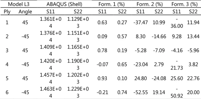
For anti-symmetric angle-ply model, only Formulation 1 leads to good results, while Formulations 2 and 3 produce inaccurate results (Table 7).

Model L3 ABAQUS (Shell) Form. 1 (%) Form. 2 (%) Form. 3 (%) Ply Angle S11 S22 S11 S22 S11 S22 S11 S22

1 45 1.361E+0 4

1.129E+0

3 0.63 0.27 -37.47 10.99

-36.00 11.94

2 -45 1.376E+0 4

1.151E+0

3 0.09 0.57 8.30 -14.66 9.28 13.44

3 45 1.409E+0 4

1.165E+0

3 0.78 0.19 -5.28 -7.09 -4.16 -5.96

4 -45 1.420E+0 4

1.190E+0

3 -0.07 0.65 -23.04 2.79

-21.73 3.82

5 45 1.457E+0 4

1.202E+0

3 0.93 0.10 24.80 -24.08 25.60 22.76

6 -45 1.463E+0 4

1.229E+0

3 -0.21 0.74 -52.55 19.14

-50.92 20.00

different formulations presented in this work. For most plies very good results were obtained, but for some plies the differences were significant. It is important to emphasize that the approaches here developed are more appropriate to symmetric laminates and antisymmetric angle-ply laminates with large number of plies.

Model L4 ABAQUS Form. 1 (%) Form. 2 (%) Form. 3 (%)

Ply Angle S11 S22 S11 S22 S11 S22 S11 S22

1 0 2.802E+0

4

4.824E+0

2 -0.39 -3.69 -0.39

-3.69 -0.39 3.69

2 90 4.779E+0 2

1.841E+0

3 15.30 -0.45 15.30

-0.45 15.30 0.45

3 0 2.896E+0

4

4.988E+0

2 -0.36 0.88 -0.36 0.88 -0.36 0.88

4 90 4.899E+0 2

1.901E+0

3 -54.64 -0.10 -54.64

-0.10 -54.64 0.10

5 0 2.990E+0

4

5.152E+0

2 -0.34 5.15 -0.34 5.15 -0.34 5.15

6 90 5.019E+0 2

1.962E+0

3 -121.23 0.24 -121.23 0.24 -121.23 0.24

Table 8 – Stress in the materials coordinates for anti-symmetric cross-ply model L4.

5 CONCLUSIONS

A simple approach combining the elementary beam theory and Classical Lamination Theory is presented to the analysis of composite laminated tubes under axial force and bending. The effective properties are computed by appropriate integration of segment properties over the tube cross section. The stresses in the material systems are evaluated using the elastic constitutive relations.

The proposed approach is much simpler than global-local procedure since it allows the structural analysis of laminated tubes using only beam elements. The proposed formulation leads to very good displacements for all lamination schemes indicating that the effective properties are accurately computed for both symmetric and non-symmetric models.

REFERENCES

Barbero, E. J., Introduction to Composite Materials Design. CRC Press, 1998.

Cook, R., Malkus, D., Plesha, M.; de Witt, R. J., Concepts and Applications of Finite Element Analysis. 4a ed., John Wiley & Sons, 2002.

Chan, W. S., and Demirhan, K. C., Simple Closed-Form Solution of Bending Stiffness for Laminated Composite Tubes. Journal of Reinforced Plastics and Composites, v. 19, pp. 278-291, 2000.

Jones, R. M., Mechanics of Composite Materials, 2ed. Philadelphia: Taylor and Francis, 1999.

Lemanski, S., and Weaver, P. Optimisation of a 4-layre laminated cylindrical shell to meet given cross-sectional stiffness properties. Composite Structures, v. 72, pp. 163-176, 2006.

Lin, C. Y., and Chan, W. S., Stiffness evaluation of elliptical laminated composite tube under bending. AIAA/ASME/ASCE/AHS/ASC Structures, Structural Dynamics and Materials Conference and Exhibit, 42nd, Seattle, WA, Apr., pp. 16-19, 2001.

Massa, J. C., and Barbero, E. J., A Strength of Materials Formulation for Thin Walled. Composite Beams with Torsion. Journal of Composite Materials, v. 32, p1560-1594, 1998.

Reddy, J. N., Mechanics of Laminated Composite Plates and Shells: Theory and Analysis, 2. ed., CRC Press, 2004.

Simulia. ABAQUS/Standard User’s Manual – Version 6.9, Providence, RI, USA, 2009.