eve asholanda Optimization of Laminated Tubes Using Finite Element Analysis

OPTIMIZATION OF LAMINATED TUBES USING FINITE ELEMENT

ANALYSIS

Rafael F. Silvaa; Iuri B. C. M. Rochaa, Evandro Parente Jr.a, Antônio M. C. Meloaand Áurea S. Holandab

a_{Departamentode Engenharia Estrutural e Construção Civil, Universidade Federal do Ceará}

Campus do Pici, Bloco 710, 60455-760, Fortaleza, Ceará, Brasil

b_{Departamentode Engenharia de Transportes, Universidade Federal do Ceará} Campus do Pici, Bloco 703, 60455-760, Fortaleza, Ceará, Brasil

Keywords: Composite materials, laminated tubes, optimization, Finite Element Method.

Abstract. This work presents a methodology for minimum weight design of laminated composite tubes. The design variables are the number of plies and the thickness and fiber orientation of each ply. The formulation includes stress and stability constraints. Multiple loading cases can be considered. A highly efficient axi-symmetric finite element formulation was developed and implemented for structural analysis. The stresses in the material system are used to compute the safety factor of the laminate using an appropriate failure criterion. The design optimization is performed using a sequential quadratic programming (SQP) algorithm. The proposed methodology is successfully applied to the design optimization of laminated composite tubes subjected to internal and external pressure, axial load and torsion. Several application examples are presented.

1 INTRODUCTION

Fiber Reinforced Composites (FRC) research and use have been rising in the recent years, due to its high specific stiffness and specific strength. Also, it features good corrosion resistance, thermal insulation, good damping performance and long fatigue life. Such features have led many industries to fund researches on the area, particularly the oil drilling and aerospace industries. Particularly, development of lighter composite tubes for fluid transportation and pressure vessels for fluid storage are on the rise. Comparative studies between steel and composite tubes for oil drilling (risers) are showed in Beyle et al. (1997).

Among many types of FRC, the use of laminated composite structures is growing widely in the last few years. This is due to the possibility of a more optimized structural design, utilizing the great tailorability it offers, since the number, orientation and sequence of plies (or laminas) can be optimized to give the exact desired structural behavior (Azarafza et al., 2009). Laminated composites consist of a series of laminae, each one consisting of unidirectional fibers embedded in a polymeric matrix, the latter transmitting the stresses between the former. (Jones, 1999;Mendonça, 2005). Design of such structures shows many complexities, as many design choices have to be made, such as the number of lamina and the thickness and orientation angle of each laminae.

A traditional design methodology can be used through the trial-and-error process, which can be an arduous process if applied to fiber reinforced composites, due its many design variables. Therefore, design of such structures is better fit to the use of optimization techniques (Vanderplaats, 2001).

The design variables can be continuous, as in Park et al. (2005), or discrete, as in Topal (2009). No unique optimum solution is usually obtained when minimum thickness is searched and the ply thicknesses are discrete variables, e.g. multiple of a basic layer thickness (Gurdal et al., 1999). In this case, it is often better to use a multi-objective optimization formulation (Marler and Arora, 2004; Silva et al., 2009; Walker and Smith, 2003). Usually, the weight of the laminate and another performance parameter is considered (Almeida and Awruch, 2009;

Topal, 2009; Deka et al., 2005). When continuous nature is used to design variables a single weight function can be used. Although the discrete nature for design variables is in general a practice requirement the use of continuous treatment is important to investigate the behavior of the solutions in a free condition with respect this constraint.

In any design optimization process, the structural security of each trial laminate has to be measured. To this end, stresses and strains in each laminae are needed, and a structural analysis procedure have to be undertaken. The combination of fiber and matrix can be modeled as an orthotropic material, with each layer being stronger in the direction of its fibers and weaker in the transversal directions. Due to the high complexity in modeling laminated composite tubes, computer programs based on numerical methods, such as the Finite Element Method (FEM), are often used.

24 degrees of freedom previously implemented in the open-code finite element program FEMOOP (Rocha et al., 2009). Also, some examples are presented comparing results with a Classical Lamination Theory solution (Silva et al., 2009) and the commercial finite element software ABAQUS (Simulia, 2007).

With stresses and strains in each laminae, various failure criteria for composite materials can be used. In turn, such criteria can yield the safety factor for the whole laminate, in a First Ply Failure fashion. In the present work, two criteria, the maximum stress and Tsai-Wu, were used.

Several algorithms have been used to the laminated optimization problem such as classical

mathematic programming techniques (Walker and Hamilton, 2006) and evolutionary

altorithms (Spallino et al., 2002) with special attention to genetic algorithms (Azarafza et al., 2009; Walker and Smith, 2003; Lemanski et al., 2001; Silva et al., 2009). The first class of methods has been successfully applied to problems with continuous variables and the last ones with discrete variables and discontinuous and nondifferentiable functions.

This work presents a simple methodology for minimum weight design of laminated tubes. Only symmetric laminates are considered. The design variables are the number of plies and the thickness and fiber orientation of each ply on the half of the laminate. All of them are treated as continuous variables. The formulation includes stress and stability constraints. Multiple load cases can be considered combining internal and external pressure, axial force and torsional moment. A highly efficient axi-symmetric finite element formulation was developed and implemented for structural analysis. The stresses in the material system are used to compute the safety factor of the laminate using an appropriate failure criterion. A sequential quadratic programming (SQP) method is used to solve the nonlinear problem.

2 STRESS ANALYSIS

An efficient finite element formulation was developed in order to compute the stresses in thick-walled laminated tubes of fiber reinforced composites. Only axisymmetric loading (internal and external pressure, axial force and torsional moment) are considered, thus bending is not allowed. The tubes are subjected to constant loads and have a large length, as a consequence the strains do not vary along the axial direction and the tube is in a Generalized Plane Strain (GPS) state.

2.1 Constitutive relations

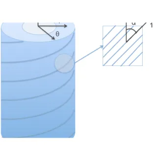
In a macroscopic scale, each lamina (or ply) can be modeled as an orthotropic material, with greater strength and stiffness in the fiber direction. Thus, the mechanical properties and stress-strain relations are described in a local (material or ply) coordinate system (1, 2, 3), where the 1-axis is parallel to the fibers, the 2-axis is perpendicular to the fibers and the 3-axis is perpendicular to the lamina. Thus, the material system is different for each ply.

On the other hand, the equilibrium equations and kinematic relations should be written in the same coordinate system for the whole structure. A global cylindrical coordinate system (r,

Figure 1 – Global and local coordinate systems.

Fiber reinforced composites can be modeled as elastic-linear until very close to failure (Jones, 1999). This, the relation between stresses (σ) and strains (ε) in the local coordinate system (1, 2, 3) can be written as

1 1 23 13 12 33 22 11 23 13 12 3 2 23 1 13 2 32 2 1 12 3 31 2 21 1 23 13 12 33 22 11 1 0 0 0 0 0 0 1 0 0 0 0 0 0 1 0 0 0 0 0 0 1 0 0 0 1 0 0 0 1 σ S ε = ⇒                     ⋅                                   − − − − − − =                     τ τ τ σ σ σ ν ν ν ν ν ν γ γ γ ε ε ε G G G E E E E E E E E E (1)

where S is the compliance matrix and the subscript 1 indicates the local system. Since this matrix is symmetric there are only 9 independent constraints. Thus:

Ejνij =Eiνji (2)

The inversion of Eq. (1) leads to:

1 1 23 13 12 3 2 1 66 55 44 33 23 13 23 22 12 13 12 11 23 13 12 3 2 1 0 0 0 0 0 0 0 0 0 0 0 0 0 0 0 0 0 0 0 0 0 0 0 0 ε C σ = ⇒                                         =                     γ γ γ ε ε ε τ τ τ σ σ σ C C C C C C C C C C C C (3)

13 32 21 13 31 32 23 21 12 23 66 13 55 12 44 21 12 3 33 31 12 32 2 23 31 13 2 22 32 21 31 1 13 23 31 21 1 12 32 23 1 11 2 1 ; ; ; 1 ; ; 1 ; ; ; 1 υ υ υ υ υ υ υ υ υ υ υ υ υ υ υ υ υ υ υ υ υ υ υ υ − − − − = ∆ = = = ∆ − ⋅ = = ∆ + ⋅ = ∆ − ⋅ = ∆ + ⋅ = ∆ + ⋅ = ∆ − ⋅ = G C G C G C E C E C E C E C E C E C (4)

Strains can be transformed from the local to the global system using (Cook et al., 2002): ε

T

ε₁ = (5)

where the transformation matrix T is given by

                    + + + + + + + + + = 2 3 3 2 2 3 3 2 2 3 3 2 3 2 3 2 3 2 3 1 1 3 3 1 1 3 3 1 1 3 1 3 1 3 1 3 1 2 2 1 1 2 2 1 1 2 2 1 2 1 2 1 2 1 3 3 3 3 3 3 2 3 2 3 2 3 2 2 2 2 2 2 2 2 2 2 2 2 1 1 1 1 1 1 2 1 2 1 2 1 2 2 2 2 2 2 2 2 2 n m n m l n l n m l m l n n m m l l n m n m l n l n m l m l n n m m l l n m n m l n l n m l m l n n m m l l n m l n m l n m l n m l n m l n m l n m l n m l n m l T (6)

In this equation mi, ni and li are the director cosines of the local axes in respect to the global axes, which are presented in Table 1.

l m n

1 0 sin α cos α

2 0 -cos α sin α

3 1 0 0 Table 1 – Director cosines.

Using the Virtual Work Principle it can be shown that stresses are transformed by

σ =TTσ_{1 (7)}

Using Eqs. (3), (5), and (7) the stress-strain relation in the global system can be written as

σ = Cε ⇒ C = TTCT (8)

where C is the constitutive matrix in the global system. Substituting the data from Table 1 in Eq. (8) leads to

σr

σ_θ σ_z τrθ

τrz

τzθ

                    =

C11 C12 C13 0 0 C14

C12 C22 C23 0 0 C24

C13 C23 C33 0 0 C34

0 0 0 _C66 C56 0

0 0 0 _C56 C55 0

C14 C24 C34 0 0 C44

                    ⋅ εr ε_θ ε_z γrθ

γrz

γθz

                    (9)

other hand, the normal and shear stresses are uncoupled for cross-ply laminations (α = 0o or 90o).

2.2 Strains and stresses

The three-dimensional strain-displacement relations in cylindrical coordinates are given by (Timoshenko and Goodier, 1970):

ε_rr = ∂u

∂r γzθ =

∂v

∂z+

1

r

∂w

∂θ   

ε_θθ = 1

r

∂v

∂θ +u 

  γzr =

∂w

∂r +

∂u

∂z

ε_zz = ∂w

∂z γθr =

1

r

∂u

∂θ −v+r ∂v

∂r



 

(10)

where u is the radial displacement, v is the out-of-plane (i.e. tangential) displacement and w is the vertical displacement. Considering only tubes subjected to axisymmetric loads (pressure, axial force and torsional moment), the strains do not depend on θ and Eq. (10) simplifies to

εrr =

∂u

∂r εθθ =

u

r εzz =

∂w ∂z γzθ =

∂v

∂z γzr =

∂w ∂r +

∂u

∂z γθr =

∂v ∂r −

v r

(11)

Considering a Generalized Plain Strain (GPS) state, the strains are constant along the length of the tube (Herakovich, 1998). Thus, the displacement fields can be written as:

z z

r w

z r z r v

r u z r u

a ε β = = =

) , (

) , (

) ( ) , (

(12)

where β is the rate of twist and εa is the axial strain, which are both constants. According to

Eqs. (11) and (12), γzr and γθr vanish and the strain-displacement relations can be written as

ε_rr = ∂u

∂r εθθ = u

r εzz =εa γθz =βr (13)

Eq. (9) shows that stresses τzr and τrθ vanish because γzr =γrθ = 0. Therefore, the stress-strain relation involving only non-zero terms is given by

σ_r σ_θ σz

τ_θz 

    



    

=

C11 C12 C13 C14

C12 C22 C23 C24

C13 C23 C33 C34

C14 C24 C34 C44



     



     

ε_r ε_θ εz

γ_θz 

    



    

(14)

C11 =C33

C12 =sin 2α

C13 + cos2α C23

C22 =sin 4

α C11 + cos4α _{C22 +} 2sin2αcos2α _C12

(

)

C13 = cos 2α

C13 + sin2α C23

C23 =sin 2

αcos2α _C11

(

)

(

)

C33 = cos 4α

C11 + sin4α _{C22 +} 2sin2α cos2α _C12

(

)

C14 =sinα cosα C13 - C23

(

)

C24 =sin 3α

cosα _{C11 - C12}

(

)

(

)

C34 =sin 3α

cosα _C12

(

)

(

)

C44 =sin 2α

cos2α _{C11 -}

(

)

(

)

(15)

2.3 Finite Element Formulation

The displacement field, Eq. (12), and the kinematic relations, Eq. (13), show that the stress analysis of long thick-walled laminated tubes subjected to axisymmetric loads is a one-dimensional problem in the radial coordinate r, since the other unknowns, β and εa, are both constants.

Therefore, the finite element formulation proposed here has only one degree of freedom per node (the radial displacement u) in addition to two global (nodeless) degrees of freedom (β and εa). In fact, the global displacement vector is given by

     

 

     

 

=

β ε_a nn

u u

M

1

u (16)

where nn is the number of mesh nodes. Thus, the finite element model has a total of 2nn+2 degrees of freedom.

The radial displacement within each finite element is interpolated from the nodal displacements ui using

u= Niui i=1

n

∑

where functions Ni are the shape functions and n is the number of element nodes. The shape

functions are Lagrange polynomials defined in parametric coordinate ξ, since only C0

continuity is required (Cook et al., 2002). Therefore, low and high order elements can be easily implemented. A sub-parametric formulation was adopted, where the radial coordinate is linearly interpolated within the element:

r=

(

)

2 r1+

1+ξ

(

)

where r1 and r2 are the radial coordinates of the first and last element nodes, respectively, as

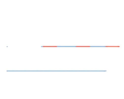
depicted in Figure 2.

Figure 2 – One-dimensional element with quadratic interpolation.

Using Eqs. (12), (13), and (17) the strains within a quadratic element can be computed from the nodal and global (nodeless) degrees of freedom:

e a a i i i i z z r u u u r r N r N r N r N r N r N r u r N u r N u B ε= ⇒                                 ∂ ∂ ∂ ∂ ∂ ∂ =                 ∂ ∂ =             β ε β ε γ ε ε ε θ θ 3 2 1 2 2 1 3 2 1 0 0 0 0 0 1 0 0 0 0 0 0 0 (19)

where B is the strain-displacement matrix and ue is the vector of element displacements, including both nodal and global degrees of freedom.

According to the Virtual Work Principle, at an equilibrium state the internal and external virtual works due to a virtual displacement field δu _{are equal:}

∫

∫

ext dV dr

W

W_int δ δ δu f

δ ε σ (20)

In the Finite Element Method the total internal work is computed by the summation of the internal work of each element:

∑∫

int δε σ

δ (21)

where ne is the number of finite elements of the model. Considering strain field ε given by

Eq. (19) and the stresses in the global system given by Eq. (8), the internal virtual work can be rewritten as:

ξ π δ

δW _e T rJd

ne e e e T e 2 1 1 1

int

∑

∫

=

= ⇒

= ₍₂₂₎

where Ke is the element stiffness matrix and J is the Jacobian of the transformation between

the radial (r) and parametric coordinates (ξ):

2 1 2 r r J d dr

J = ⇒ = −

ξ (23)

u K u u K u T ne e e e T e

W δ δ

δ =

∑

=1

int (24)

The global stiffness matrix is assembled summing up the element matrices by the standard finite element procedure (Bathe, 1996; Cook et al., 2002), but considering both nodal and global degrees of freedom of each element, according to Eqs. (16) and (19).

The external work for a tube subjected only to internal pressure (pi), external pressure (pe), axial force (N) and torsional moment (T) is given by:

f uT a nn e e i i

ext rp u r p u N T

W π δ π δ δε δβ δ

δ =2 ₁−2 + + = (25)

where ri and re are the inner and outer radius respectively. Therefore, the external force vector is simply:                       − = T N p r p r e e i i π π 2 0 0 2 M f (26)

Finally, the global equilibrium equation is obtained from Eq. (20), (24), and (25):

f

Ku= (27)

In design optimization it is important the consideration of multiple load cases. As the structural analysis is linear, the global stiffness matrix is the same for all load cases. Thus, computation implementation can handle multiple load cases, computing stresses, strains, and displacements for each of them. So, for an analysis with m load cases, the global equilibrium given by Eq. (27) takes the form:

                      − − =                       − − ) ( ) 1 ( ) ( ) 1 ( ) ( ) 1 ( ) ( ) 1 ( ) ( ) 1 ( ) ( ) 1 ( ) ( ) 1 ( ) ( 1 ) 1 ( 1 ) ( 2 ) 1 ( 2 ) ( 1 ) 1 ( 1 2 2 0 0 0 0 2 2 K m m m e e e e m i i i i m m a a m n n m n n m m T T N N p r p r p r p r u u u u u u u u L L L L M L M L L L L L L M L M L L π π π π β β ε ε (28)

where the numbers in parenthesis denote the load cases.

2.4 Local Strains and Stresses

In order to evaluate the failure of the laminate, the stresses and strains in the local coordinate system are needed. Initially, the strain field in the global system is obtained using

of Eq. (5), the following the global-local transformation should be used: ε T ε = ⇒                                 + + + =                     1 2 3 3 2 3 2 3 2 3 2 1 3 3 1 3 1 3 1 3 1 1 2 2 1 2 1 2 1 2 1 3 3 2 3 2 3 2 3 2 2 2 2 2 2 2 2 1 1 2 1 2 1 2 1 23 13 12 33 22 11 2 2 2 2 2 2 2 2 2 z z r n m n m n n m m l l n m n m n n m m l l n m n m n n m m l l n m n m l n m n m l n m n m l θ θ γ ε ε ε γ γ γ ε ε ε (29)

Finally, stresses in local system are obtained using the elastic relation in the local system,

Eq.(3).

It is well known that the finite element stresses and strains may have poor accuracy close to the element edges, i.e. at the external nodes, which are the points where stresses are generally sought. Thus, in this work the stresses are calculated in the Gauss points and extrapolated to the nodes. For the element with quadratic interpolation, the stresses are computed at the Gauss point of a 2-point quadrature and linearly extrapolated along the element using 2 3 1 2 3 1 )

( σ ₁ ξ σ ₂ ξ

σ s = _p − + _p + (30)

where ξ is the parametric coordinate and p1 and p2 are the stresses at first and second Gauss

point, respectively.

3 FAILURE CRITERIA

The stresses and strains in the local coordinate system (1, 2, 3) can be used to evaluate the structural safety of the laminate, using an appropriate failure criteria. For this purpose the applied stress and strain state are compared to those of a failure state, obtained in laboratory.

For isotropic materials, whose mechanical properties are constant in every direction, classic failure criteria such as Tresca and von Mises are extensively used. For such materials, only one strength parameter, defined by a yield or failure stress, is used and there are few failure modes.

On the other hand, for orthotropic materials, the mechanical properties vary in the three main orthogonal directions. Thus, different strength parameters have to be used for each direction. Furthermore, for fiber reinforced composites, such parameters have different values for tension and compression, with 9 independent parameters in a three-dimensional load state. The failure criteria for orthotropic materials can be applied to detect the failure of individual plies.

Laminate failure is more difficult to define than ply failure. Two criteria have been used: First Ply Failure (FPF) and Ultimate Laminate Failure (ULF). FPF considers that the laminate fails when the first ply fails. On the other hand, in ULF a progressive failure analysis is performed, in which the load is applied in a sequence of steps and the stiffness of failed plies is degraded. The load is increased until the last ply fails leading to the ultimate load.

In the present work, the First Ply Failure is adopted as the criterion to define laminate

failure and two well-known criteria, the Maximum Stress and the Tsai-Wu (Jones, 1999;

3.1 Maximum Stress Criterion

In the Maximum Stress criterion, the stress in each direction of the local (material) system is compared separately with the material strength in that direction. Therefore, there is no interaction between the stresses in different directions. In a three-dimensional analysis, the failure envelope for this criterion is represented by:

6 6

5 5

4 4

3 3

3 3

3

2 2

2 2

2

1 1

1 1

1

0 0

0 0

0 0

F F F when F

when F

when F

when F

when F

when F

c t

c t

c t

= = = 

 

< −

> =

  

< −

> =

  

< −

> =

τ τ τ

σ σ σ

σ σ σ

σ σ σ

(31)

where F1t, F1c, F2t, F2c, F3t, F3c, are the tensile (t) and compression (c) strengths and F4, F5, F6

are the shear strengths. The Safety Factor (SF) is determined as the minimum relation

between the actual stress component and the respective material strength:

      

= = =

6 , 5 , 4

3 , 2 , 1

min

i with F

i with F

SF

i i i i

τ σ

(32)

The Maximum Stress Criterion is very simple, intuitive, and easily implemented. Moreover, it allows the consideration of different strength parameters for tensile and compressive strengths and the determination of the failure mode.

3.2 Tsai-Wu Criterion

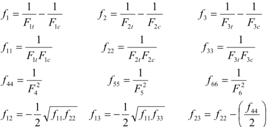
The Tsai-Wu criterion is based on the polynomial failure theory proposed by Gol'denblat and Kopnov (Daniel and Ishai, 2005). The Tsai-Wu failure surface is given by

1

= + _{ij i j}

i

i f

fσ σσ (33)

      − = − = − = = = = = = = − = − = − = 2 2 1 2 1 1 1 1 1 1 1 1 1 1 1 1 1 44 22 23 33 11 13 22 11 12 2 6 66 2 5 55 2 4 44 3 3 33 2 2 22 1 1 11 3 3 3 2 2 2 1 1 1 f f f f f f f f f F f F f F f F F f F F f F F f F F f F F f F F f c t c t c t c t c t c t (34)

The Safety Factor is then obtained using Eq. (33). The resultant expression is a second-degree polynomial equation and the Safety Factor is the positive root of this equation:

a a b b SF 2 4 2− + − = (35) where 3 3 2 2 1 1 3 2 23 3 1 13 2 1 12 2 6 66 2 5 55 2 4 44 2 3 33 2 2 22 2 1

11 2 2 2

σ σ σ σ σ σ σ σ σ σ σ σ σ σ σ f f f b f f f f f f f f f a + + = + + + + + + + + = (36)

Tsai-Wu criterion fits well the available experimental data (Barbero, 1999). In addition it is simple and easy to implement. The linear terms of Eq. (33) allow the consideration of the difference between tensile and compressive strengths. On the other hand, it does not indicate the failure mode.

4 OPTIMIZATION MODEL

This section presents the formulation for optimum design of laminated composite tubes subjected to axisymmetric loads (internal and/or external pressure, axial force, torsional moment). The tubes can be subjected to multiple load cases. The loads, material properties, number of plies (n), inner radius (Ri), and required safety factor are the input data of the optimization problem, whose aim is to find the best (lower cost) lamination for the tube. Only

symmetric laminations are considered, as depicted in Figure 3, in order to avoid some

undesired couplings.

Figure 3 – Stack sequence of a composite tube.

symmetric laminations are allowed, the vector of design variables is given by

   

  =

2 2

1 2 2

1 h hn n

h K α α K α

x (37)

These variables are subjected to lower and upper bounds:

max min

º 90 º

90

h h

h _k

k

≤ ≤

≤ ≤

− α

, k =1...n/2 (38)

The formulation aims to minimize the cost of the tube, which is assumed proportional to the volume of composite material. Since the section of the tube is assumed constant along the tube length, the volume can be represented by the cross-sectional area of the tube. A normalized value is used to improve the convergence of the optimization algorithm and the objective function (f) is given by

min max

min )

(

A A

A A f

− − =

x ₍₃₉₎

where Amin and Amax, are the minimum and maximum values of the cross-section area:

(

)

(

)

2 2 min min

max max

2 2 max max

, ,

h n R R

R R A

h n R R

R R A

i i

i i

+ = −

=

+ = −

= π π

(40)

Strength and stability constraints are considered in order to obtain a safe tube design. Thin-walled tubes subjected to external pressure can buckle as a shell due to the compressive stresses in the hoop direction (hoop buckling). The collapse pressure of long thin-walled laminated cylindrical shells (Weingarten et al., 1968; Vinson and Sierakowski, 2002) can be computed from

3

22 2 22 22

3 

  

 

− =

A B D R k

p_{col p (41)}

where R is the mean radius, D22, B22, and A22 are elements of the laminate stiffness matrix computed by the Classical Lamination Theory (Reddy, 1996; Jones, 1999; Daniel and Ishai,

2005), and kp is a knock-down factor used to consider the effects of geometrical

imperfections. Weingarten et al. (1968) suggest to use kp = 0.75 for laminated shells.

For tubes subjected to both internal (pi) and external pressure (pe), buckling can occur only

when the pressure differential (∆p), defined as

e i p

p

p= −

∆ (42)

is negative. Since the tube can be subjected to m load cases, the stability constraint can be written as

m l

p p

p

p_col ≥∆ _max, where ∆ _max=MAX(−∆ _l), =1,... ₍₄₃₎

In the computer implementation, the constraint is written in the normalized form:

0 1 max

≤ + ∆ −

p p_col

(44)

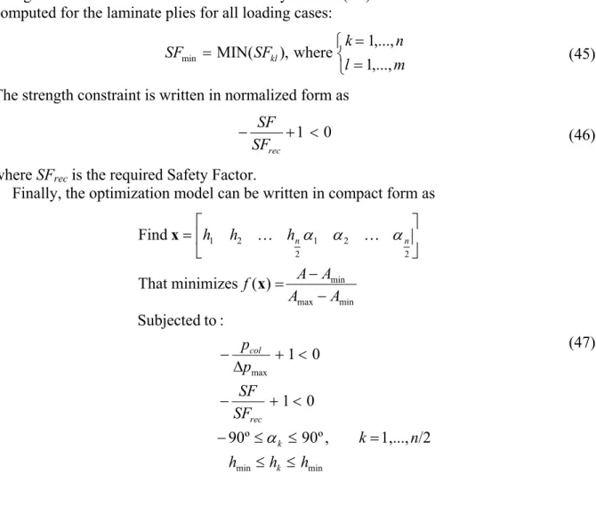
Using the FPF criterion the laminate Safety Factor (SF) is determined as the smallest SF computed for the laminate plies for all loading cases:

  

= = =

m l

n k

SF

SF _kl

,..., 1

,..., 1 where , ) ( MIN

min (45)

The strength constraint is written in normalized form as

0 1 <

+ −

rec

SF SF

(46)

where SFrec is the required Safety Factor.

Finally, the optimization model can be written in compact form as

min min

max

min max

min

2 2

1 2 2

1

/2 1,..., ,

º 90 º

90

0 1

0 1

: to Subjected

) ( minimizes That

Find

h h h

n k

SF SF

p p

A A

A A f

h h

h

k k rec col

n n

≤ ≤

= ≤

≤ −

< + −

< + ∆ −

− − =

   

  =

α

α α

α

x

x K K

(47)

5 NUMERICAL EXAMPLES

In this section, a series of numerical examples is presented. Initially, two sets of finite element examples are presented, validating the proposed analysis model. Later, a number of optimization examples are presented.

5.1 Analysis Examples

Before using the implemented analysis method in design optimization, some examples will be presented in order to confirm the validity of its results in local stresses. The material used in the model was the T300 Graphite-Epoxy, whose properties are presented below:

E1(GPa) E2(GPa) E3(GPa) G12(GPa) G13(GPa) G23(GPa) ν12 ν13 ν23

141.6 10.7 10.7 5.7 5.7 3.4 0.268 0.268 0.495

Table 2 – Material properties for the T300 Graphite-Epoxy.

The first set of examples was presented in Xia et al. (2001), where three lamination schemes were subjected to internal pressure. In the present workr the global stresses were

compared with the analytical solution implemented by Herakovich (1998) in the MathCad

thickness is 2 mm, and the applied internal pressure is 10 MPa. The lamination schemes and results are presented below:

Lay-up r z θ zθ

[55/-55/55/-55] Face (kPa) (kPa) (kPa) (kPa) Internal -1.00E+04 1.46E+03 2.57E+05 1.23E+05 Herakovich

External 7.28E-12 -1.28E+03 2.44E+05 -1.12E+05 Internal -1.00E+04 1.47E+03 2.57E+05 1.23E+05 FEMOOP (2D)

External 7.19E-01 -1.35E+03 2.44E+05 -1.12E+05 Internal -1.00E+04 1.46E+03 2.57E+05 1.23E+05 Unidimensional

External 6.95E-01 -1.28E+03 2.44E+05 -1.12E+05 Table 3 – Results for Layup 1.

Layup _{r z θ zθ}

[55/-55/30/-30] Face (kPa) (kPa) (kPa) (kPa) Internal -1.00E+03 -7.51E+03 -1.84E+04 -6.73E+03 Herakovich

External -1.01E+04 7.49E+03 -4.98E+03 -5.53E+03 Internal -1.00E+04 1.35E+05 4.50E+05 2.47E+05 FEMOOP (2D)

External 2.46E-01 -1.34E+05 5.31E+04 4.82E+04 Internal -1.00E+04 1.35E+05 4.50E+05 2.46E+05 Unidimensional

External 2.37E-01 -1.34E+05 5.31E+04 4.81E+04 Table 4 – Results for Layup 2.

Layup _{r z θ zθ}

[55/-30/30/-55] Face (kPa) (kPa) (kPa) (kPa) Internal -1.00E+04 1.38E+05 4.58E+05 2.52E+05 Herakovich

External -1.16E-10 1.29E+05 4.32E+05 -2.33E+05 Internal -1.00E+04 1.38E+05 4.59E+05 2.52E+05 FEMOOP (2D)

External 1.20E+00 1.29E+05 4.32E+05 -2.33E+05 Internal -1.00E+04 1.38E+05 4.58E+05 2.52E+05 Unidimensional

External 1.15E+00 1.29E+05 4.32E+05 -2.33E+05 Table 5 – Results for Layup 3.

Although direct comparison with the results in Xia et al., 2001 is not accurate since no numerical data was given, there is good concordance with the graphical data presented in the paper. Also, comparison between the two-dimensional and one-dimensional finite elements yielded good results.

Comparing the results with the analytical solution also yielded good results, except in lay-up 2. However, the obtained analytical results are clearly illogical, since the radial stress in the internal face of the tube is 10 times smaller than the applied internal pressure and does not drop to zero in the external face, as no external pressure was applied. Such matter will be further investigated.

internal area of the tube, are applied. Also, one of the examples features an internal steel liner, whose properties are presented in Table 6.

E (GPa) ν G (GPa) Fa (GPa) Fs (GPa)

200 0.30 76.9 0.577 0.333

Table 6 – Mechanical properties of steel.

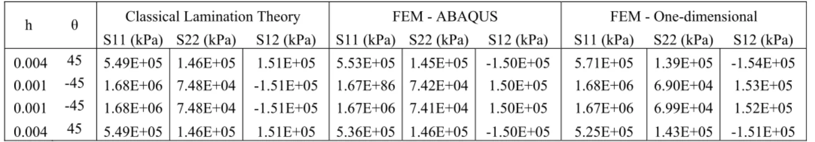
In ABAQUS, the tubes were modeled with 3m length and using S8R thick shell elements with reduced integration. The results for 3 different layups are presented below, this time with stresses in the local system.

Classical Lamination Theory FEM - ABAQUS FEM – One-dimensional h θ

S11 (kPa) S22 (kPa) S12 (kPa) S11 (kPa) S22 (kPa) S12 (kPa) S11 (kPa) S22 (kPa) S12 (kPa) 0.002 55 5.78E+05 4.27E+04 2.15E+04 5.73E+05 4.24E+04 -2.14E+04 5.86E+05 3.38E+04 -2.30E+04 0.002 -55 5.78E+05 4.27E+04 -2.15E+04 5.73E+05 4.24E+04 2.14E+04 2.81E+05 3.49E+04 2.26E+04 0.002 -55 5.78E+05 4.27E+04 -2.15E+04 5.73E+05 4.24E+04 2.14E+04 5.76E+05 3.60E+04 2.23E+04 0.002 55 5.78E+05 4.27E+04 2.15E+04 5.73E+05 4.24E+04 -2.14E+04 5.72E+05 3.70E+04 -2.20E+04 0.002 Liner 7.18E+05 1.34E+06 0.00E+00 7.12E+05 1.33E+06 0.00E+00 6.97E+05 1.32E+06 0.00E+00

Table 7 – Results for Layup 4.

Classical Lamination Theory FEM - ABAQUS FEM - One-dimensional h θ

S11 (kPa) S22 (kPa) S12 (kPa) S11 (kPa) S22 (kPa) S12 (kPa) S11 (kPa) S22 (kPa) S12 (kPa) 0.004 90 7.36E+05 1.03E+05 0.00E+00 7.30E+05 1.02E+05 0.00E+00 7.48E+05 9.39E+04 0.00E+00 0.001 0 1.10E+06 7.96E+04 0.00E+00 1.09E+06 7.89E+04 0.00E+00 1.09E+06 7.46E+04 0.00E+00 0.001 0 1.10E+06 7.96E+04 0.00E+00 1.09E+06 7.89E+04 0.00E+00 1.09E+06 7.43E+04 0.00E+00 0.004 90 7.36E+05 1.03E+05 0.00E+00 7.30E+05 1.02E+05 0.00E+00 7.20E+05 9.84E+04 0.00E+00

Table 8 – Results for Layup 5.

Classical Lamination Theory FEM - ABAQUS FEM - One-dimensional h θ

S11 (kPa) S22 (kPa) S12 (kPa) S11 (kPa) S22 (kPa) S12 (kPa) S11 (kPa) S22 (kPa) S12 (kPa) 0.004 45 5.49E+05 1.46E+05 1.51E+05 5.53E+05 1.45E+05 -1.50E+05 5.71E+05 1.39E+05 -1.54E+05 0.001 -45 1.68E+06 7.48E+04 -1.51E+05 1.67E+86 7.42E+04 1.50E+05 1.68E+06 6.90E+04 1.53E+05 0.001 -45 1.68E+06 7.48E+04 -1.51E+05 1.67E+06 7.41E+04 1.50E+05 1.67E+06 6.99E+04 1.52E+05 0.004 45 5.49E+05 1.46E+05 1.51E+05 5.36E+05 1.46E+05 -1.50E+05 5.25E+05 1.43E+05 -1.51E+05

Table 9 – Results for Layup 6.

The results for the last 3 layups show good concordance. The difference in the signal of S12 in layups 1 and 3 is due only to sign convention and is not detrimental to the analysis, as the sign of shear stresses is irrelevant in the calculation of failure criteria. Layup number 4 also demonstrates the versatility of the implemented analysis model, permitting the use of multiple materials.

5.2 Optimization Examples

For each trial layup, the maximum number of plies was fixed at 4, with minimum thickness fixed at 1 mm. The lamination angle interval was fixed between -90º and 90º. Also, the internal radius was taken as 0.30m. The table below shows the material properties used in the examples.

E1 (GPa) E2 (GPa) E3 (GPa) ν12 ν13 ν23 G12 (GPa) G13 (GPa) G23 (GPa)

117 8 8 0.34 0.34 0.49 5.70 5.70 3.40

F1t (GPa) F1c (GPa) F2t (GPa) F2c (GPa) F3t (GPa) F3c (GPa) F4 (GPa) F5 (GPa) F6 (GPa)

1.64 1.28 0.08 0.25 0.08 0.25 0.1 10 10 Table 10 – Material properties of Graphite-Epoxy.

Initially, to validate the implemented optimization formulation, classic load cases were tested. In all of them, the final layup agreed with the applied loads. In the axial force, internal pressure and torque cases, the objective function was restricted by the safety factor. In the external pressure case, the collapse pressure was the active restriction.

Design Variables Constraints Load

h (m) Angle (deg) SF pcol

Fobj Area (m2)

N = 20MN [0.002154 / 0.001046]s [0 / 0]s 1.000 - 0.110 0.0122 pi = 20MPa [0.002007 / 0.001917]s [63.581 / -45.724]s 1.000 - 0.146 0.0150

pe = 5MPa [0.001152 / 0.008273]s [90 / 90]s 5.507 5,00E+06 0.429 0.0366

T = 3MNm [0.003386 / 0.002827]s [43.922 / -43.682]s 1.000 - 0.263 0.0239 Table 11 – Results for simple loads.

The next set of examples used multiple load cases, represented by Scenarios A and B. In

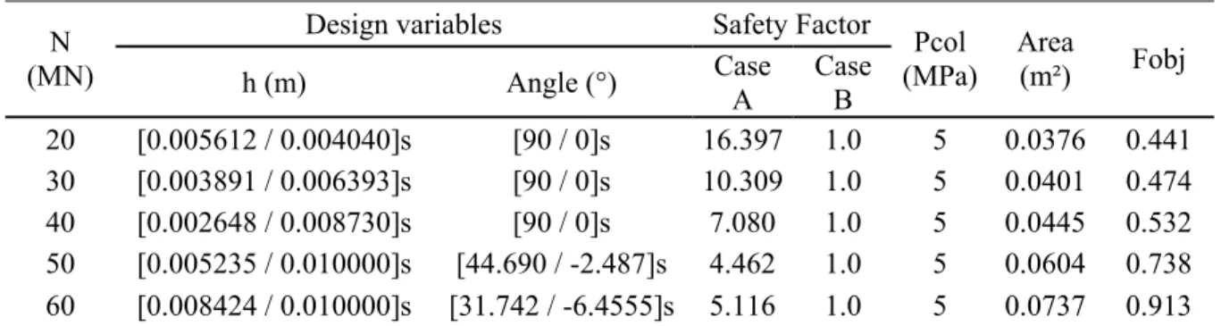
Table 12, scenario A was a fixed internal pressure of 5MPa. Case B consists of an axial force with variable value. Raising the axial force causes an increase in the thickness of the tube, decreasing the safety factor of Tsai-Wu for Scenario A. In all of the cases, the collapse pressure restriction was active. So, in Case A, the strength constraint is activated, and in Case B, the buckling constraint is activated. The same happens in Table 13 and 14.

Design variables Safety Factor N

(MN) _{h (m) Angle (°)} Case

A

Case B

Pcol (MPa)

Area (m²) Fobj 20 [0.005612 / 0.004040]s [90 / 0]s 16.397 1.0 5 0.0376 0.441 30 [0.003891 / 0.006393]s [90 / 0]s 10.309 1.0 5 0.0401 0.474 40 [0.002648 / 0.008730]s [90 / 0]s 7.080 1.0 5 0.0445 0.532 50 [0.005235 / 0.010000]s [44.690 / -2.487]s 4.462 1.0 5 0.0604 0.738 60 [0.008424 / 0.010000]s [31.742 / -6.4555]s 5.116 1.0 5 0.0737 0.913

Design variables Safety Factor pi

(Mpa) _{h (m) Angle (deg)} Case

A

Case B

Pcol (MPa)

Area (m²) Fobj 20 [0.008429 / 0.001000]s [90 / +-20.497]s 7.162 1.0 5 0.0367 0.429 30 [ 0.008160 / 0.001265]s [90 / 0]s 10.797 1.0 5 0.0367 0.429 40 [ 0.007372 / 0.002086]s [90 / 0]s 14.966 1.0 5 0.0368 0.431 50 [0.005814 / 0.003936]s [±81.759 / m16.788]s 16.694 1.0 5 0.0380 0.446 60 [0.005752 / 0.005682]s [±62.408 / m47.258]s 18.639 1.0 5 0.0448 0.535

Table 13 – Case A: Fixed External Pressure (Pext = 5Mpa) e Case B: Variable Internal Pressure.

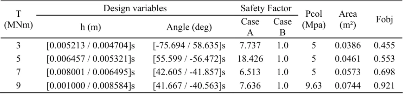
Design variables Safety Factor T

(MNm) _{h (m) Angle (deg)} Case

A

Case B

Pcol (Mpa)

Area (m²) Fobj 3 [0.005213 / 0.004704]s [-75.694 / 58.635]s 7.737 1.0 5 0.0386 0.455 5 [0.006457 / 0.005321]s [55.599 / -56.472]s 18.426 1.0 5 0.0461 0.553 7 [0.008001 / 0.006495]s [42.605 / -41.857]s 6.513 1.0 5 0.0573 0.698 9 [0.001000 / 0.008584]s [41.667 / -40.563]s 7.636 1.0 9.63 0.0744 0.921

Table 14 – Case A: Fixed External Pressure (Pext = 5Mpa) e Case B: Variable Torque.

In Table 15,two constraints related to Tsai-Wu Failure are activated. While Case A leads to layup [+65º / -45º]s, the axial force leads to [0º / 0º]s (Table 11). The Axial Force varying from 20MN to 40MN in Case B does not produce a substantial increase in 90º plies thickness. However, the number of 0º plies increase considerably. The constraints related to Tsai-Wu criterion are activated in both load cases.

Design variables Safety Factor N

(MN) _{h (m) Angle (deg)} Case

A

Case B

Area (m²) Fobj 20 [0.001823 / 0.004361] [90 / 0] 1.0 1.0 0.0238 0.261 30 [0.001683 / 0.006619] [±89.958 / m0.003] 1.0 1.0 0.0322 0.370 40 [0.001544 / 0.008877] [±89.732 / m0.009] 1.0 1.0 0.0407 0.481 50 [0.008230 / 0.010000] [±58.781 / m1.613] 1.0 1.0 0.0729 0.902

Table 15 – Case A: Fixed Internal Pressure (Pint = 20Mpa) e Case B: Variable Axial Force.

In Table 16, the internal pressure is maintained fixed, while external pressure is varied. The Tsai-Wu constraint is activated in Case A, but not in Case B. However, the stability constraint related is active. It can be noted that while the external pressure increases from 5 to 30 MPa, the orientation angles of internal plies increases too. While the external pressure rises, the fiber orientation tends to 90º to eliminate the hoop buckling.

Design variables Safety Factor pe

(MPa) _{h (m) Angle (deg)} Case

A Case B

Pcol (Mpa)

Area (m²) Fobj 5 [0.008429 / 0.001000]s [90 / ±20.497]s 1.0 7.1622 5 0.0367 0.429 10 [0.010000 / 0.001988]s [±89.892 / m38.041]s 1.0 4.0048 10 0.0470 0.564 15 [0.010000 / 0.003845]s [±89.198 / m51.465]s 1.0 2.7035 15 0.0546 0.663 20 [0.010000 / 0.005326]s [±88.352 / m62.725]s 1.0 2.0658 20 0.0607 0.743 25 [0.010000 / 0.006546]s [±88.123 / m73.240]s 1.0 1.6907 25 0.0658 0.809 30 [0.008498 / 0.009081]s [90 / 90]s 1.002 1.4449 30 0.0702 0.866

Table 16 – Case A: Fixed Internal Pressure (Pint = 20Mpa) e Case B: Variable External Pressure.

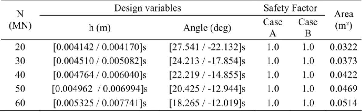
Design variables Safety Factor N

(MN) _{h (m) Angle (deg)} Case

A

Case B

Area (m²) 20 [0.004142 / 0.004170]s [27.541 / -22.132]s 1.0 1.0 0.0322 30 [0.004510 / 0.005082]s [24.213 / -17.854]s 1.0 1.0 0.0373 40 [0.004764 / 0.006040]s [22.219 / -14.855]s 1.0 1.0 0.0422 50 [0.004962 / 0.006994]s [20.425 / -12.944]s 1.0 1.0 0.0469 60 [0.005325 / 0.007741]s [18.265 / -12.019]s 1.0 1.0 0.0514

Table 17 – Case A: Fixed Torque (T = 3 MNm) e Case B: Variable Axial Force

6 CONCLUSIONS

The simplified unidimensional finite element analysis model showed good results in all

comparisons. Results were compared with two analytical formulations (Herakovich, 1998;

Silva et al., 2009) and with finite element package ABAQUS all showed great concordance. Such results show that the consideration of a Generalized Plain Strain state (GPS) is reasonable to analyze tubes subjected to axi-symmetric loads. In comparison with the

axisymmetric analysis model implemented in FEMOOP (Rocha et al., 2009), which had 24

degrees of freedom per element, the results were nearly identical. Therefore, with only 3 radial degrees of freedom per element and 2 global ones, such element is very efficient, and therefore suitable to usage with optimization techniques. In the analytical solution provided by Herakovich (1998), layup 2 provided unreasonable results, which asks for further tests and investigation of the matter. However, the other layups showed good results.

Various composite tubes models are successfully optimized, showing the robustness of the proposed formulation. Initially, four basic models of composite tubes are optimized leading to the classical solutions. Axial Force leads to 0º fibers angles, Torque to [+45 / -45º], combating maximum stresses in principal directions related to shearing. Internal pressure produces approximately (+65º / -45). External pressure leads to [90º / 90º] combating hoop buckling.

REFERENCES

Almeida, F. S., Awruch, A. M., Design Optimization of Composite Laminated Structures Using Genetic Algorithms and Finite Element Analysis. Composite Structures, v. 88, pp. 443-454, 2009.

Azarafza, R., Khalili, S. M. R., Jafari, A. A., Davar, A., Analysis and optimization of laminated composite circular cylindrical Shell subject to compressive axial and transverse transient dynamics loads. Thin-Walled Structures, vol. 47, pp. 970-983, 2009.

Bathe, K. J., Finite Element Procedures. Prentice Hall, 1996.

Barbero, E. J., Introduction to Composite Material Design, CRC Press, 1999.

Beyle, A. I., Gustafson C. G., Kulakov, V. L., & Tarnopol’skii, Y. M. Composite risers for deep-water offshore technology: Problems and prospects. 1. Metal-Composite riser. Mechanics of Composite Materials, vol33, n. 5, pp. 577-591, 1997.

Cook, R., Malkus, D., Plesha, M.; de Witt, R. J., Concepts and Applications of Finite Element Analysis. John Wiley & Sons, 2002.

Daniel, I. M., Ishai, O., Engineering Mechanics of Composite Materials, 2nd edition. Oxford University Press, 2005.

Deka, D. J., Sandeep, G., Chakraborty, D., & Dutta, A., Multiobjective optimization of

laminated composites using finite element method and genetic algorithm. Journal of

reinforced Plastics and Composites, vol. 24, pp. 273, 2005.

Gurdal, Z., Haftka, R. T., Hajela, P., Design and Optimization of Laminated Composite

Materials. John Wiley, 1999.

Herakovich, C. T., Mechanics of Fibrous Composites. John Wiley & Sons, 1998. Jones, R. M., Mechanics of Composite Materials, 2nd Ed. Taylor and Francis, 1999.

Lemanski, S. L., Hill, G. F. J. Weaver, P. M., The relative merits of genetic algorithms in the

optimization of laminated cylindrical shells. 3rd ASMO Conference on Engineering

Design Optimization, 2001.

Marler, R. T., Arora, J. S., Survey of multi-objective optimization methods for engineering. Structural and Multidisciplinary Optimization, vol. 26, pp. 369-395, 2004.

Mendonça, P. T. R., Materiais Compósitos e Estruturas Sanduíches - Projeto e Análise.

Editora Manole, 2005.

Park, J. H., Hwang, J. H., Lee, C. S., Hwang, W., Stacking sequence design of composite laminates for maximum strength using genetic algorithms. Composite Structures, v. 52, pp 217-231, 2001.

Reddy, J. N., Mechanics of Laminated Composite Plates: Theory and Analysis. CRC Press,

1996.

Rocha, I. B. C. M; Parente Jr, E.; Melo, A. M. C.; Holanda, A. S., A Finite Element Formulation for Composite Tube Modeling. Procedures of the 30th CILAMCE, 2009. Silva, R. F.; Melo, A. M. C.; Parente Jr, E., Projeto Preliminar de Tubos Compósitos via

Algoritmos Genéticos. Procedures of the 30th CILAMCE, 2009.

Simulia, ABAQUS/Standard User's Manual - Version 6.7, Providence, RI, USA, 2007.

Spallino, R., & Rizzo, S., Multi-objective optimization of laminated structures. Mechanics Research Communications, vol. 29, pp. 17-25, 2002.

Timoshenko, S. P; Goodier, J. N., Theory of Elasticity, 3rd Edition. McGraw-Hill Kogakusha Ltd, 1970.

Topal, U., Multiobjective optimization of laminated composite cycindrical shells for

maximum frequency and buckling load. Materiais and Design, vol 30, pp. 2584-2594,

Vanderplaats, G. N., Numerical Optimization Techniques for Engineering Design. Vanderplaats Research and Development, 2001.

Vinson, J. R.; Sierakowski, R. L., The Behavior of Structures Composed of Composite

Materials. Kluwer Academic Publishers, 2002.

Walker, M., Hamilton, R., A technique for optimally designing fibre-reinforced laminated plates under in-plane loads for minimum weight with manufacturing uncertainties accounted for. Engineering with Computers, vol. 21, pp. 282-288, 2006.

Walker, M., Smith, R. E., A technique for the multiobjective optimisation of laminated composite structures using genetic algorithms and finite element analysis. Composite Structures, vol. 62, pp. 123-128, 2003.

Weingarten, V. I.; Seide, P.; Peterson, J. P., Buckling of Thin-Walled Circular Cylinders. NASA SP 8007, Space Vehicle Design Criteria (Structures), 1968