Spatial variation of modelled and measured NO, NO<sub>2</sub> and O<sub>3</sub> concentrations in the polluted urban landscape – relation to meteorology during the Göte-2005 campaign

(1)

ACPD

9, 2081–2111, 2009

Modelled and measured NO, NO2

and O₃in the urban landscape

J. Klingberg et al.

Title Page

Abstract Introduction

Conclusions References

Tables Figures

◭ ◮

Back Close

Full Screen / Esc

Printer-friendly Version

Interactive Discussion

Atmos. Chem. Phys. Discuss., 9, 2081–2111, 2009 www.atmos-chem-phys-discuss.net/9/2081/2009/ © Author(s) 2009. This work is distributed under the Creative Commons Attribution 3.0 License.

Atmospheric Chemistry and Physics Discussions

This discussion paper is/has been under review for the journalAtmospheric Chemistry

and Physics (ACP). Please refer to the corresponding final paper inACPif available.

Spatial variation of modelled and

measured NO, NO

₂

and O

₃

concentrations

in the polluted urban landscape – relation

to meteorology during the G ¨ote-2005

campaign

J. Klingberg1, L. Tang2, D. Chen2, G. Pihl Karlsson3, E. B ¨ack4, and H. Pleijel1

1

Department of Plant and Environmental Sciences, University of Gothenburg, P.O. Box 461, 405 30 Gothenburg, Sweden

2

(2)

ACPD

9, 2081–2111, 2009

J. Klingberg et al.

Title Page

Tables Figures

◭ ◮

Back Close

Full Screen / Esc

3

Swedish Environmental Research Institute (IVL), P.O. Box 5302, 400 14 Gothenburg, Sweden

4

City of Gothenburg, Environmental Administration, Karl Johansgatan 23, 414 59 Gothenburg, Sweden

Received: 6 November 2008 – Accepted: 3 December 2008 – Published: 22 January 2009

Correspondence to: J. Klingberg (jenny.klingberg@dpes.gu.se)

(3)

ACPD

9, 2081–2111, 2009

J. Klingberg et al.

Title Page

Tables Figures

◭ ◮

Back Close

Full Screen / Esc

Interactive Discussion Abstract

Knowledge about temporal and spatial variations of the O₃and NO_xrelationship in the urban environment are necessary to assess the exceedance of air quality standards for NO₂. Both reliable measurements and validated high-resolution air quality models are important to assess the e_ffect of tra_ffic emission on air quality. In this study,

measure-5

ments of NO, NO₂and O₃concentrations were performed in Gothenburg, Sweden, dur-ing the G ¨ote-2005 campaign in February 2005. The aim was to evaluate the variation of pollutant concentrations in the urban landscape in relation to urban air quality mon-itoring stations and wind speed. A brief description of the meteorological conditions and the air pollution situation during the G ¨ote-2005 campaign was also given.

Further-10

more, the Air Pollution Model (TAPM) was used to simulate the NO_x-regime close to an urban tra_ffic route and the simulations were compared to the measurements. Im-portant conclusions were that the pollutant concentrations varied substantially in the urban landscape and the permanent monitoring stations were not fully representative for the most polluted environments. As expected, wind speed strongly influenced

mea-15

sured pollutant concentrations and gradients. Higher wind speeds dilute NO₂ due to stronger dispersion; while at the same time vertical transport of O₃is enhanced, which produces NO₂ through oxidation of NO. The oxidation e_ffect was predominant at the more polluted sites, while the dilution effect was more important at the less polluted sites. TAPM reproduced the temporal variability in pollutant concentrations

satisfacto-20

rily, but was not able to resolve the situation at the most polluted site, due to the local scale site-specific conditions.

1 Introduction

It is well documented that nitrogen dioxide (NO₂) and ozone (O₃) can adversely a_ffect human health (Curtis et al., 2006). In the European Union Framework Directive on Air

25

(4)

ACPD

9, 2081–2111, 2009

J. Klingberg et al.

Title Page

Tables Figures

◭ ◮

Back Close

Full Screen / Esc

(1999/30/EC) limit values for nitrogen dioxide (NO₂) concentration are defined as an hourly average of 200µg m−3₍

∼105 nmol mol−1, 99.8-percentile) and an annual aver-age of 40µg m−3₍

∼21 nmol mol−1), to be achieved by 1 January 2010. Measurements and modelling indicate that many urban areas will have problems to reach the air quality standard for NO₂, especially close to major tra_ffic routes (Carslaw et al., 2007; Pleijel

5

et al., 2009).

The levels of NO₂and O₃are closely linked by the chemical coupling of O₃with NO_x (NO₂₊NO). O₃levels are generally lower at ground level in streets than at rooftops or in the surrounding countryside due to the titration of O₃ by NO in car exhaust to form NO₂(Fenger, 1999). Therefore reductions of NO_xemissions in the cities are frequently

10

accompanied by an increase in the level of O₃. A better understanding of the relation-ships between O₃, NO and NO₂, as well as the influence of the state of the atmosphere is necessary to evaluate the exceedances of air quality standards (Clapp and Jenkin, 2001). In addition, both for air quality forecasting and for development of control strate-gies it is important to identify the factors controlling the NO₂ concentrations (Shi and

15

Harrison, 1997).

The spatial variability of air pollutants is large in urban areas (Coppalle et al., 2001; Vardoulakis et al., 2005). Therefore exposure to air pollutants is strongly dependent on location. Cost, bulk of equipment, power supply, etc. often put practical limits to the number of air quality monitoring stations in a city. In many cities air pollutants are only

20

measured at one or a few locations. It is therefore very important to assess the repre-sentativeness of these locations (Flemming et al., 2005). How far from traffic routes the local impact of traffic emissions reaches and to which amount these emissions affect the formation or destruction of ozone is not well known (Suppan and Sch ¨adler, 2004). Both measurements and validated high resolution air quality model calculations are

25

(5)

ACPD

9, 2081–2111, 2009

J. Klingberg et al.

Title Page

Tables Figures

◭ ◮

Back Close

Full Screen / Esc

Progresses in fine scale meteorological and air chemistry modelling over the last decades have made it possible to fairly realistically model urban air pollution dynam-ics. One such model is The Air Pollution Model (TAPM), which is a three-dimensional, nestable, prognostic meteorological and air pollution model. Previous studies have shown that TAPM performs well in coastal, inland and complex terrain, in sub-tropical to

5

mid-latitude conditions (Hurley et al., 2001, 2003, 2005). Chen et al. (2002) evaluated the meteorological performance of TAPM in Gothenburg, Sweden for a two year long meteorology only simulation. The results showed that meteorological variables from TAPM were in agreement with observations on yearly and daily time scales. A recent model intercomparison study between TAPM and MM5 (the PSU/NCAR mesoscale

10

model) carried out in Gothenburg concluded that TAPM is comparable to MM5 and has better performance in urban areas (Tang et al., 2009), in terms of surface meteoro-logical variables including temperature and wind which are important to air pollution dynamics. While TAPM’s ability to realistically reproduce local meteorological condi-tions have been demonstrated and the simulacondi-tions have been successfully used in

15

urban air pollution studies (e.g. Johansson et al., 2008), its capability in reproducing local scale variability in pollutant concentrations has been tested to a lesser extent.

The measurements and modelling in this study formed part of the G ¨ote-2005 campaign (http://www2.chem.gu.se/∼_{hallq/Gote eng 2005.htm), which took place in}

Gothenburg, South-West Sweden, from 2 February to 2 March, 2005. The

coordi-20

nation of di_fferent research groups’ measurements created a platform for cooperation and a common database with measurement data. Through coordination of unique competences, the overall goals of the G ¨ote-2005 campaign were to (1) better describe the air pollution situation in Gothenburg, (2) increase the understanding of the fate of the air pollutants near the road, (3) provide a base for risk assessment, (4) test new

25

measurement techniques and (5) evaluate air pollution models.

The objectives of the part of the G ¨ote-2005 campaign described in the present paper were:

(6)

ACPD

9, 2081–2111, 2009

J. Klingberg et al.

Title Page

Tables Figures

◭ ◮

Back Close

Full Screen / Esc

the G ¨ote-2005 campaign.

– Evaluate how the NO, NO₂and O₃concentrations varied in the urban landscape compared to permanent monitoring stations. The hypothesis was that there is a large spatial (and temporal) variability within the city, not fully resolved by the monitoring stations.

5

– Investigate how the NO₂ concentrations varied with wind speed at differently pol-luted sites. The hypothesis was that the influence of wind speed/turbulence on NO₂concentrations is a balance between increased dilution and enhanced verti-cal transport of O₃to oxidize NO to NO₂.

– Compare the observations with results from the TAPM model. The hypothesis was

10

that the model simulations would correlate well with the corresponding observa-tions, but not necessarily be able to reproduce dynamics at sites with very high pollution levels due to local scale variations in the site-specific characteristics.

2 Material and methods

2.1 Air pollution and meteorological measurements

15

Measurements of NO, NO₂ and O₃ concentrations were performed using passive dif-fusion samplers of the IVL type (Ferm, 2001) during five 5-day intervals from 2 to 27 February 2005, at eight different locations in Gothenburg. In addition, temperature (T) and relative humidity (RH) were measured with Tinytag (INTAB Interface-Teknik AB) sensors/loggers TGP 1500 (recording every 10 min) enclosed in self-ventilating

radia-20

(7)

ACPD

9, 2081–2111, 2009

J. Klingberg et al.

Title Page

Tables Figures

◭ ◮

Back Close

Full Screen / Esc

and elevations in relation to this major traffic route, including a site in a nearby park. One site was co-located with the urban rooftop monitoring site Femman, which per-mitted comparison of passive sampler and Tinytag data with continuously operating monitors and meteorological observations (T and RH with Campbell Rotronic MP101 and wind speed with Gill Ultrasonic). One further site was a rural reference (Annek ¨arr)

5

situated about 25 km north-east of the Gothenburg city centre. If not stated otherwise,

the measurement height was 2 m for the passive samplers and 1.5 m for T and RH

measurements with Tinytags. At Femman, O₃ concentration was measured with an

UV absorption monitor (Monitor Labs 9811), NO_x with a Tecan CLD 700 AL and PM₁₀

with a TEOM 1400A. Further continuous NO and NO₂ data (Opsis DOAS system)

10

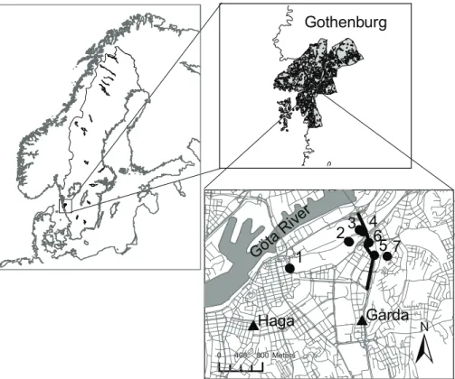
were received from a measurement station nearby the major tra_ffic route (G ˚arda) and a measurement station situated in a city street environment (Haga). The location of the measurement sites can be seen on the map in Fig. 1. Coordinates and further characteristics of the measurement sites are given in Table 1.

2.2 Evaluation of passive samplers and Tinytag data

15

One week before and three weeks after the measurement period the Tinytags, in their self-ventilated radiation shields, were kept at Femman in parallel with the Rotronic sensor, the latter expected to provideT and RH with high accuracy, for calibration. After correction a relationship close to 1:1 was obtained between the di_fferent Tinytags and the Rotronic forT. For example, the relationship between the Tinytag co-located with

20

the Femman Rotronic the entire measurement period was T_Rotronic₌T_Tinytag₊0.00004, R2₌0.95. Calibration of RH close to 100% was complicated. Below 80% there was a relationship close to 1:1, but values above 80% could not be accurately corrected for all Tinytags because of occasional out of range values. One Tinytag was lost (stolen, site 2) after the second measurement period.

25

(8)

ACPD

9, 2081–2111, 2009

J. Klingberg et al.

Title Page

Tables Figures

◭ ◮

Back Close

Full Screen / Esc

of the NO, NO₂ and O₃ samplers from the Femman instrument measurements were

25%, 5% and 1%, respectively. For reasons unknown, the NO samplers did not work properly at Annek ¨arr suggesting very high concentrations at this rural site. Therefore NO values from this site were excluded.

2.3 TAPM configurations

5

The meteorology module of TAPM predicts the local scale flow, such as sea breezes and terrain induced circulation given the larger scale synoptic meteorological fields. The mean horizontal wind components are determined from the momentum equations and the terrain-following vertical velocity from the continuity equation. The air pollu-tion module of TAPM consists of an Eulerian grid-based set of prognostic equapollu-tions for

10

pollutant concentrations. Gas-phase photochemistry is based on the semi-empirical mechanism called the generic reaction set (GRS) of Azzi et al. (1992), with the hy-drogen peroxide modification of Venkatram et al. (1997). See Hurley (2005) for more details, including reactions, the specification of reaction rates and yield coefficients. In this study, TAPM was run from 2 to 27 February 2005 with three nested domains of

15

41×41 horizontal grid points at 10, 3, 1 km spacing for the meteorology and 31×51 horizontal grid (N-S direction by E-W direction) points at 1.0, 0.3, 0.1 km spacing for air pollution. All domains centred at the location (57◦₄₂′_{N, 11}◦₅₈′_{E, Site 1/Femman in}

Fig. 1) and the innermost domains consist of the Gothenburg city centre. The lowest ten of the 40 vertical levels were 10, 25, 50, 75, 100, 150, 200, 250, 300, 350 m a.g.l.,

20

with the highest model level at 8000 m a.g.l. The initial and boundary conditions used for TAPM was six-hourly synoptic scale analyses at 1.0 degree in latitude and longitude spacing from the Australian Bureau of Meteorology. Observed winds at J ¨arnbrott (ap-proximately 7 km south-west of Gothenburg city centre) were assimilated as nudging terms and assuming a 10 km radius of influence, which improved the wind simulation.

25

(9)

ACPD

9, 2081–2111, 2009

J. Klingberg et al.

Title Page

Tables Figures

◭ ◮

Back Close

Full Screen / Esc

domain data available from the US Geological Survey. The monthly sea-surface tem-perature was extracted from model default database based on US National Centre for Atmospheric Research (NCAR) (http://dss.ucar.edu/datasets). Monthly varying deep soil volumetric moisture content was set to 0.38 m3m−3from the European Centre for Medium-Range Weather Forecasts (www.ecmwf.int).

5

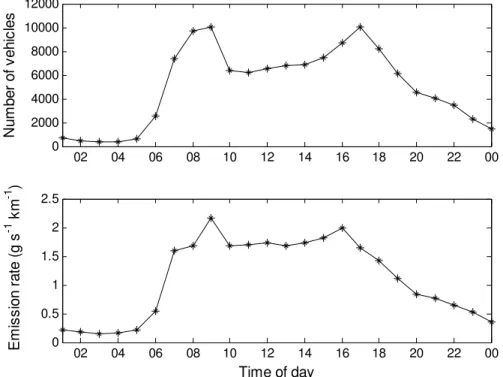
The traffic route passing through Olskroksmotet, located in the north-east of the city centre, is one of the busiest roads in Gothenburg (see Fig. 1). Data on the number of vehicles and their average speed on the highway were received from the Swedish National Road Administration’s website (www.vv.se). Estimated emission fac-tors for NO_xbased on the Swedish National Road Administration’s information system

10

EVA 2.2 were received from the City of Gothenburg, Environmental Administration. Thereafter the emission rate of NO_x for each hour of the day was calculated (Fig. 2). Carslaw (2005) has found evidence of an increasing NO₂/NO_x emissions ratio from about 5–6 vol% in 1997 to about 17 vol% in 2003 in London. Pleijel et al. (2009) in-vestigated the NO₂/NO_xemission ratio in Gothenburg and found it to be approximately

15

15 vol%, which was used in this study.

In this study, the hourly NO₂ and O₃ concentrations at the Femman rooftop moni-toring site were used as urban background values. Emissions of volatile organic com-pounds (VOC) were not considered in this study since there is generally insufficient time available for reactions including VOC to become important on the small

geograph-20

ical scale of a few kilometres (Carslaw and Beevers, 2005). However, the urban back-ground of VOC was given by setting the smog reactivity,R_smogas 0.5 nmol mol−1in the model. As a result, TAPM predicted the hourly average for NO₂, NO_xand O₃provided with the estimated emission rate of NO_x at Olskroksmotet.

To evaluate the TAPM against the observations the explained variance (R2) was

25

calculated:

R2=1− P

(obs_i₋pred_i)2

P

(10)

ACPD

9, 2081–2111, 2009

J. Klingberg et al.

Title Page

Tables Figures

◭ ◮

Back Close

Full Screen / Esc

where obs represents observations and pred the corresponding prediction. An R2

close to 1 means a small deviation from the 1:1 line. Also a linear regression (y₌kx₊m) was made between model and observations. The explained variance according to the regression (r2) is always higher than R2. Ifr2 is significantly higher thanR2there is a systematic error in the model.

5

3 Results

Table 2 describes the meteorological conditions during night and day, separately for weekdays and weekends, and for the total G ¨ote-2005 period. For the interpretation of air pollution data it was important to know that no systematic meteorological di_ff er-ences between weekdays and weekends had arisen by unfortunate coincidence. There

10

were no major differences in meteorology between weekdays and weekends during the measurement period. In general, the G ¨ote-2005 campaign was characterised by rel-atively cloudy and windy weather, with partial snow cover. Temperature inversions were not strongly developed during the campaign. Consequently, air pollution con-centrations did not grow very large. For example, NO never reached concon-centrations

15

higher than 316 nmol mol−1 at rooftop level (Femman), 550 nmol mol−1 at G ˚arda and 307 nmol mol−1at Haga during G ¨ote-2005, while this pollutant reached 670 nmol mol−1 at Femman during an inversion episode in February 2004 (Janh ¨all et al., 2006).

Table 3 shows the mean concentration of air pollutants during night and day, sepa-rately for weekdays and weekends, and for the total G ¨ote-2005 period. It is clear that

20

the concentrations of NO and NO₂ were higher on weekdays compared to weekends

during daytime also at rooftop level, emphasizing the important impact of the tra_ffic. As

a consequence, the O₃ concentrations were lower on weekdays compared to

week-ends, due to stronger titration of O₃ by NO in weekdays. The Swedish air quality standard for NO₂of 90µg m−3(∼47 nmol mol−1) averaged over an hour was exceeded

25

(11)

ACPD

9, 2081–2111, 2009

J. Klingberg et al.

Title Page

Tables Figures

◭ ◮

Back Close

Full Screen / Esc

of exceedances was larger. At the G ˚arda monitoring site the air quality standard for NO₂ was exceeded 11.5% (80 h) of the hours and at the Haga monitoring site 5.3% (37 h) of the hours during the G ¨ote-2005 period. In general the PM₁₀ concentrations were low during the period except for an episode in the end of February with the max-imum concentration of 212µg m−3 _{during one hour. It was the only day during the}

5

period when the air quality standard of 50µg m−3 averaged over a day was exceeded (64µg m−3).

3.1 NO, NO₂and O₃concentrations in relation to location of monitoring site

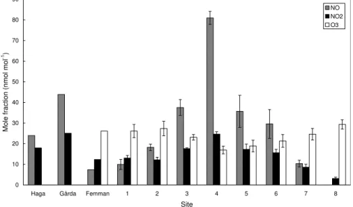
Figure 3 shows the mean variation in O₃, NO and NO₂ concentrations between the different sites during the measurement period. The Femman monitoring site was

rela-10

tively low in NO and NO₂compared to most of the other urban sites, with the exception of the park site. For instance, the 25-day average of NO₂was 13.1 nmol mol−1_at

Fem-man, while 24.7 nmol mol−1 _{at the site closest to the tra}

ffic route. The rural site was however much lower in NO₂ compared to the urban sites, only 3.1 nmol mol−1. The variation of NO in the urban landscape was larger. Concentrations of NO at the most

15

polluted site (site 4) were approximately eight times higher than at the Femman rooftop monitoring station and nearly twice as high as at the G ˚arda monitoring station. For NO₂, being largely a secondary pollutant, the concentration at the most polluted site was twice as high as the urban background, Femman, and for O₃ the concentration was approximately 30% lower in the most polluted site compared to Femman. There

20

was a clear negative effect of NO emissions on the O₃concentration at the most pol-luted sites, while the variation in O_x (NO₂₊O₃) between sites was relatively small, the range being between 32.4 nmol mol−1at the rural site and 41.6 nmol mol−1at the most polluted site.

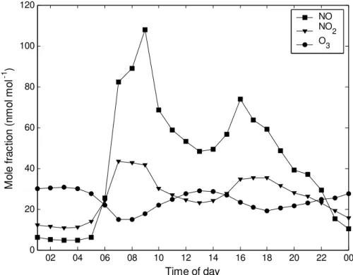
The diurnal variation in the NO/NO₂ system di_ffered substantially between the

25

(12)

ACPD

9, 2081–2111, 2009

J. Klingberg et al.

Title Page

Tables Figures

◭ ◮

Back Close

Full Screen / Esc

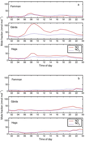
weekdays the diurnal cycle at G ˚arda was characterized by two peaks of NO concen-tration corresponding to the morning and afternoon rush hours. The morning peak was larger due to less air mixing at this time of the day than at the afternoon peak. The morning peak during weekdays can also be seen at Femman and Haga. Less traffic, which was more evenly distributed over the day, resulted in no pronounced peaks and

5

in NO₂ concentrations larger compared to the NO concentration during large parts of the day during weekends.

3.2 TAPM simulations

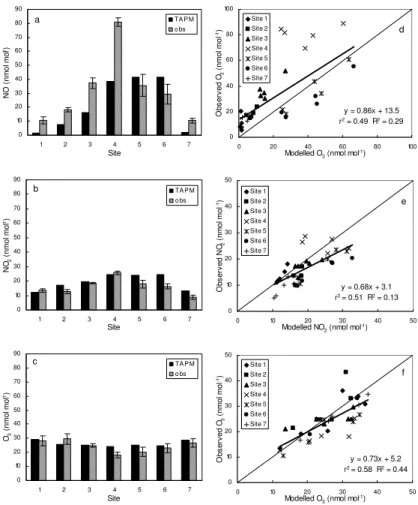
Figure 5 presents the modelled and observed mean NO, NO₂ and O₃ concentations

at the seven sites close to the traffic route (Olskroksmotet) during the G ¨ote-2005

pe-10

riod. The O₃concentration showed the best agreement between the model simulation and observations with aR2 of 0.44. The TAPM tended to overestimate NO₂. The NO concentration showed more scattering and therefore a lowerR2. The passive sampler detection limit for NO is higher compared to NO₂ and O₃, which could be an explana-tion for the large intercept of the regression line between observed and modelled NO

15

concentration in Fig. 5d. TAPM successfully reproduced the relationship between NO_x and O₃observed by the passive samplers. The highest NO_xconcentrations were found closest to the emissions at the tra_ffic route. The model also showed the lowest O₃ con-centrations close to the road due to NO titration. Figure 6 shows the modelled diurnal cycle of NO, NO₂and O₃at site 6 (the most NO polluted site according to TAMP) which

20

was also satisfactorily reproduced. Two peak daily values of NO and NO₂correspond to two tra_ffic rush hours with large emissions. The O₃ concentrations were lowest at peak NO_xconcentrations.

3.3 Spatial variation of air pollutants in relation to wind speed

The di_fference in O₃ concentration between the most polluted site 4 and the rooftop

25

(13)

ACPD

9, 2081–2111, 2009

J. Klingberg et al.

Title Page

Tables Figures

◭ ◮

Back Close

Full Screen / Esc

with wind speed. The concentration difference was larger at higher wind speeds. The O₃ concentration increased with wind speed at both sites, but the increase was more rapid at Femman, reflecting a stronger coupling with the more O₃rich air layers aloft at that site and the larger consumption of O₃in reaction with NO at the more polluted site. The e_ffect of wind speed on the NO₂concentration ratio of the polluted urban landscape

5

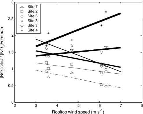
and the Femman rooftop monitoring site is shown in Fig. 7. Higher wind speeds act to dilute NO₂ due to stronger dispersion, but also lead to an enhanced vertical transport of O₃, which produces NO₂ through oxidation of NO. The oxidation e_ffect dominated at the two most polluted sites, while the dilution e_ffect was more important at the less polluted sites.

10

A similar pattern was found when looking at the modelled data. Figure 8 shows the average NO₂ ratio between the di_fferent sites and the Femman monitoring site di-vided into wind speed classes. The sites have been ranked depending on how NO polluted they were according to the model. The least polluted site 7 had approximately the same level of NO₂ as the Femman monitoring site rather independently of wind

15

speed. At the more polluted sites the NO₂ concentration was 1.5 times that of Fem-man in calm or windy conditions. At medium wind speeds of 2 to 3 m s−1 the NO₂ ratio ([NO₂]_{site 4}/[NO₂]_Femman) increased to 3 at the most polluted sites. At higher wind speeds dispersion was the dominating process also at the most polluted sites. In the class with the highest wind speeds (6–7 m s−1) the average NO₂ratio increased again.

20

(14)

ACPD

9, 2081–2111, 2009

J. Klingberg et al.

Title Page

Tables Figures

◭ ◮

Back Close

Full Screen / Esc

Interactive Discussion 4 Discussion

4.1 Spatial and temporal variation in pollutant concentration

The results clearly indicated large spatial and temporal variations in pollutant concen-trations even though the windy weather situation during the measurement period did not promote extreme differences between locations. One way of describing the spatial

5

representativeness of measurement sites is the concept of air quality regimes. Pro-nounced di_fferences in magnitude and range of observed concentrations at di_fferent sites can be considered as different regimes of air quality. Flemming et al. (2005) identified six di_fferent air quality regimes (from “rural” to “severely polluted street”) by hierarchical clustering based on the medians of daily means from measured NO₂ at

10

400 monitoring sites in Germany during 1995–2001. The G ˚arda monitoring site of the present study was similar to the severely polluted urban environments in Germany with typical daily averages above 60µg m−3 _{(Flemming et al., 2005). The pronounced}

di-urnal cycle with two daily maxima during morning and evening rush hour also placed G ˚arda in Flemming’s severely polluted street category. The Femman and Haga

mon-15

itoring stations were comparable to Flemming’s urban and polluted urban categories, respectively. The NO concentrations followed the amount of traffic more closely than NO₂and therefore varied more between measurement sites. Fenger (1999) also found that the NO concentration follows the amount of tra_ffic more closely than NO₂, the con-centration of which is partly determined by the available O₃ supplied from outside the

20

city to oxidise NO.

The increasing O₃concentration with increasing distance from the tra_ffic route was in agreement with measurements in Toronto, Canada (Beckerman et al., 2008). Accord-ing to Sillman (1999) significant removal of O₃ during daytime occurs in the vicinity of large NO emission sources (through the reaction NO₊O₃_→NO₂₊O₂), where the NO_x

25

(15)

ACPD

9, 2081–2111, 2009

J. Klingberg et al.

Title Page

Tables Figures

◭ ◮

Back Close

Full Screen / Esc

in O₃ concentrations closest to the traffic route where the NO_x concentration reached 50 nmol mol−1 _{or higher. At the most polluted site (site 4) the reduction in O}

3

concen-tration was on average 10 nmol mol−1compared to urban background, which is in the same range as what Suppan and Sch ¨adler (2004) found in a modelling study of the impact of highway emissions on ozone in Germany. At the same time our

measure-5

ments showed a doubling in NO₂ concentration at the most polluted site compared to urban background which was in agreement with the results of Palmgren et al. (1996) from Copenhagen.

4.2 Performance of TAPM

It has been demonstrated that the TAPM can be a tool to investigate the impacts of

10

meteorological conditions on air pollutants at regional and urban scales. The results in this study showed that the model was able to reproduce the daily variations of NO, NO₂ and O₃ concentrations at local scale. However, the air pollution module of TAPM, with the smallest resolution of 100 m, restricts the performance of the model at a specific site near the tra_ffic route. The NO concentration west of the tra_ffic route (site 1 to 3) was

15

underestimated by TAPM which might be due to the fact that emissions from nearby roads and other emission sources were not included in the TAPM simulations. The di_fference between modelled and measured air pollutant concentrations was largest for NO at site 4. This site was located only 8 m from the traffic route in the road canyon which restricted air mixing and dispersion of air pollutants. The measurements at this

20

site showed a very high concentration on NO which is likely to be very local and site-specific. A drawback in the comparison of measurements and TAPM was that the measurements and model simulations did not have the same time-resolution. While the TAPM simulations gave hourly concentrations the measurements only had a time-resolution of five days. Furthermore, in order to obtain good model results, a

high-25

(16)

ACPD

9, 2081–2111, 2009

J. Klingberg et al.

Title Page

Tables Figures

◭ ◮

Back Close

Full Screen / Esc

4.3 Wind speed and NO_x-O₃interactions

Many factors influence the NO_xand O₃concentrations in the urban landscape. Based on measurements of NO_x, O₃ and meteorology, Shi and Harrison (1997) developed a model to analyze and predict NO_xand NO₂concentrations in London. They found that primary emissions and wind speed were the most important factors influencing NO_x

5

concentration. In addition, the reaction of NO with O₃ was a major factor influencing NO₂concentrations.

The measurements in this study clearly indicated that the NO₂ concentration in re-lation to urban background responded differently to increasing wind speed depending on the degree of pollution at the site. At the most polluted sites the NO₂concentration

10

ratio increased with increasing wind speed while at the least polluted sites the NO₂ concentration ratio decreased. Due to the limited amount of data the correlations were not statistically significant but the same pattern was shown by TAPM. Two processes are of importance and in delicate balance. Higher wind speeds act to dilute NO₂due to stronger dispersion, but also lead to an enhanced vertical transport of O₃, which

pro-15

duces NO₂through oxidation of NO. Palmgren et al. (1996) found the background O₃ level to be the limiting component for the occurrence of high levels of NO₂in Danish ur-ban streets. In the urur-ban background in Denmark the limiting component for formation of NO₂was often the available amount of NO and not O₃as in the streets.

The results shown in this paper illustrates the complexity of the temporal and

spa-20

tial air pollution variations in the urban landscape. The importance of measurements and knowledge about the measurement site characteristics and representativeness are emphasized. Also it has been shown that TAPM has the potential to be an impor-tant tool in evaluating air quality problems in Gothenburg and other cities with similar characteristics.

(17)

ACPD

9, 2081–2111, 2009

J. Klingberg et al.

Title Page

Tables Figures

◭ ◮

Back Close

Full Screen / Esc

Interactive Discussion 5 Conclusions

Important conclusions from the present study were:

– The G ¨ote-2005 campaign was characterised by relatively cloudy and windy

weather resulting in no strongly developed temperature inversions. Consequently, air pollution concentrations did not grow very large during the campaign.

5

– The most polluted site had considerably higher levels of NO_x, especially the pri-mary pollutant NO, compared to the urban rooftop continuous monitoring station Femman. The most polluted site also had considerably higher levels of NO com-pared to the most polluted continuous monitoring site, G ˚arda. Thus the perma-nent monitoring stations were not fully representative for the most polluted

envi-10

ronments in Gothenburg.

– Pollutant concentrations and pollutant gradients in the urban landscape were strongly dependent on the wind speed. The effect of wind on NO₂ concentra-tion in urban areas was a delicate balance between stronger dispersion at high wind speeds (diluting NO₂) and enhanced vertical transport of O₃to oxidize NO

15

to NO₂ by stronger winds. The latter effect was strongest at more polluted sites, while the first dominated at less polluted sites.

– TAPM reproduced the relation of NO, NO₂ and O₃ satisfactorily as well as the site differences under different wind speed. However, TAPM was not able to re-solve the NO situation at the most polluted site, due to local scale site-specific

20

conditions.

Acknowledgements. Thanks to Mattias Hallquist who coordinated the G ¨ote-2005

measure-ment campaign and thereby created many appreciated research cooperation opportunities. The Gothenburg Atmospheric Science Center (GAC) is gratefully acknowledged for financial support.

(18)

ACPD

9, 2081–2111, 2009

J. Klingberg et al.

Title Page

Tables Figures

◭ ◮

Back Close

Full Screen / Esc

Interactive Discussion References

Azzi, M., Johnson, G., and Cope, M.: An introduction to the generic reaction set photochemi-cal smog mechanism, in: Proceedings of the 11th International Clean Air and Environment Conference, Clean Air Society of Australia and New Zealand, Brisbane, Australia, 5–10 July 1992, 451–462, 1992.

5

Beckerman, B., Jerrett, M., Brook, J. R., Verma, D. K., Arain, M. A., and Finkelstein, M. M.: Correlation of nitrogen dioxide with other traffic pollutants near a major expressway, Atmos. Environ., 42, 275–290, 2008.

Carslaw, D. C.: Evidence of an increasing NO2/NOxemissions ratio from road traffic emissions,

Atmos. Environ., 39, 4793–4802, 2005.

10

Carslaw, D. C. and Beevers, S. D.: Estimations of road vehicle primary NO2exhaust emission

fractions using monitoring data in London, Atmos. Environ., 39, 167–177, 2005.

Carslaw, D. C., Beevers, S. D., and Bell, M. C.: Risks of exceeding the hourly EU limit value for nitrogen dioxide resulting from increased road transport emissions of primary nitrogen dioxide, Atmos. Environ., 41, 2073–2082, 2007.

15

Chen, D., Wang, T., Haeger-Eugensson, M., Aschberger, C., and Borne, K.: Application of TAPM in Swedish West Coast: Modelling results and their validation during 1999–2000, IVL report L02/51, 2002.

Clapp, L. J. and Jenkin, M. E.: Analysis of the relationship between ambient levels of O3, NO2

and NO as a function of NOx in the UK, Atmos. Environ., 35, 6391–6405, 2001.

20

Coppalle, A., Delmas, V., and Bobbia, M.: Variability of NOxand NO2concentrations observed

at pedestrian level in the city centre of a medium sized urban area, Atmos. Environ., 35, 5361–5369, 2001.

Curtis, L., Rea, W., Smith-Willis, P., Fenyves, E., and Pan, Y.: Adverse health effects of outdoor air pollutants, Environ. Int., 32, 815–830, 2006.

25

Fenger, J.: Urban air quality, Atmos. Environ., 33, 4877–4900, 1999.

Ferm, M.: Validation of a diffusive sampler for ozone in workplace atmospheres according to EN838, in: Proceedings of the International conference on measuring air pollutants by diffusive sampling, Montpellier, France, 26–28 September 2001, 298–303, 2001.

Flemming, J., Stern, R., and Yamartino, R. J.: A new air quality regime classification scheme

30

for O3, NO2, SO2and PM10observations sites, Atmos. Environ., 39, 6121–6129, 2005.

(19)

pol-ACPD

9, 2081–2111, 2009

J. Klingberg et al.

Title Page

Tables Figures

◭ ◮

Back Close

Full Screen / Esc

lution model for year-long predictions in the Kwinana industrial region of Western Australia, Atmos. Environ., 35, 1871–1880, 2001.

Hurley, P. J., Manins, P., Lee, S., Boyle, R., Ng, Y. L., and Dewundege, P.: Year-long, high-resolution, urban airshed modelling: verification of TAPM predictions of smog and particles in Melbourne, Australia, Atmos. Environ., 37, 1899–1910, 2003.

5

Hurley, P. J.: The air pollution model (TAPM) ver. 3. Part 1: Technical description. CSIRO, Australia, ISBN–0643068910, 2005.

Hurley, P. J., Physick, W. L., and Luhar, A. K.: TAPM: A practical approach to prognostic mete-orological and air pollution modelling, Environ. Modell. Softw., 20, 737–752, 2005.

Janh ¨all, S., Olofson, K. F. G., Andersson, P. U., Pettersson, J. B. C., and Hallquist, M.: Evolution

10

of the urban aerosol during winter temperature inversion episodes, Atmos. Environ., 40, 5355–5366, 2006.

Johansson, M., Galle, B., Yu, T., Tang, L., Chen, D., Li, H., Li, J. X., and Zhang, Y.: Quantifica-tion of total emission of air pollutants from Beijing using mobile mini-DOAS, Atmos. Environ., 42, 6926–6933, 2008.

15

Palmgren, F., Berkowicz, R., Hertel, O., and Vignati, E.: Effects of reduction of NOxon the NO2

levels in urban streets, Sci. Total Environ., 189–190, 409–415, 1996.

Pleijel, H., Klingberg, J., and B ¨ack, E.: Characteristics of NO2pollution in the city of

Gothen-burg, south-west Sweden – relation to NOx and O3 levels, photochemistry and monitoring

location, Water Air Soil Poll., Focus, doi:10.1007/s11267-008-9201-y, 2009.

20

Shi, J. P. and Harrison, R. M.: Regression modelling of hourly NOx and NO2concentrations in

urban air in London, Atmos. Environ., 31, 4081–4094, 1997.

Sillman, S.: The relation between ozone, NO_x and hydrocarbons in urban and polluted rural environments, Atmos. Environ., 33, 1821–1845, 1999.

Suppan, P. and Sch ¨adler, G.: The impact of highway emissions on ozone and nitrogen

ox-25

ide levels during specific meteorological conditions, Sci. Total Environ., 334–335, 215–222, 2004.

Tang, L., Miao, J. F., and Chen, D.: Performance of TAPM against MM5 at urban scale during G ¨OTE2001 campaign, Boreal. Environ. Res., 14, online: http://www.borenv.net/BER/pdfs/ preprints/Tang.pdf, 2009.

30

(20)

ACPD

9, 2081–2111, 2009

J. Klingberg et al.

Title Page

Tables Figures

◭ ◮

Back Close

Full Screen / Esc

Vardoulakis, S., Gonzales-Flesca, N., Fisher, B. E. A., and Pericleous, K.: Spatial variability of air pollution in the vicinity of a permanent monitoring station in central Paris, Atmos. Environ., 39, 2725–2736, 2005.

Venkatram, A., Karamchandani, P., Pai, P., Sloane, C., Saxena, P., and Goldstein, R.: The de-velopment of a model to examine source-receptor relationships for visibility on the Colorado

5

(21)

ACPD

9, 2081–2111, 2009

J. Klingberg et al.

Title Page

Tables Figures

◭ ◮

Back Close

Full Screen / Esc

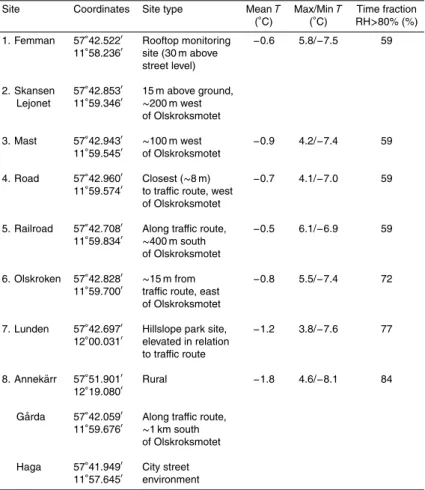
Interactive Discussion Table 1. Site names, coordinates, site characteristics, mean, maximum and minimum

tem-perature (T, ◦_{C) and the fraction of time (%) with relative humidity (RH) above 80% based on}

measurements with Tinytags.

Site Coordinates Site type MeanT Max/MinT Time fraction (◦_C) ₍◦_C) _RH_>_{80% (%)}

1. Femman 57◦_42.522′ _{Rooftop monitoring} ₋_0.6 _5.8/₋_7.5 ₅₉

11◦_58.236′ _{site (30 m above}

street level) 2. Skansen 57◦_42.853′ _{15 m above ground,}

Lejonet 11◦_59.346′

∼200 m west of Olskroksmotet

3. Mast 57◦_42.943′ _∼_{100 m west} ₋_0.9 _4.2/₋_7.4 ₅₉

11◦_59.545′ _{of Olskroksmotet}

4. Road 57◦_42.960′ _{Closest (}_∼_{8 m)} ₋_0.7 _4.1/₋_7.0 ₅₉

11◦_59.574′ _{to tra}_ffi_{c route, west}

of Olskroksmotet

5. Railroad 57◦_42.708′ _{Along tra}_ffi_{c route,} ₋_0.5 _6.1/₋_6.9 ₅₉

11◦_59.834′

∼400 m south of Olskroksmotet 6. Olskroken 57◦_42.828′

∼15 m from −0.8 5.5/−7.4 72

11◦_59.700′ _tra_ffi_{c route, east}

of Olskroksmotet 7. Lunden 57◦_42.697′ _{Hillslope park site,}

−1.2 3.8/−7.6 77 12◦_00.031′ _{elevated in relation}

to traffic route 8. Annek ¨arr 57◦_51.901′ _Rural

−1.8 4.6/−8.1 84 12◦_19.080′

G ˚arda 57◦_42.059′ _{Along tra}_ffi_{c route,}

11◦_59.676′ _∼_{1 km south}

of Olskroksmotet Haga 57◦_41.949′ _{City street}

(22)

ACPD

9, 2081–2111, 2009

J. Klingberg et al.

Title Page

Tables Figures

◭ ◮

Back Close

Full Screen / Esc

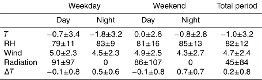
Interactive Discussion Table 2. Mean and standard deviation of temperature (T,◦_{C), relative humidity (RH, %), wind}

speed (wind, m s−1

) and global radiation (radiation, W m−2

) during the G ¨ote-2005 campaign (2 February to 2 March) based on measurements at rooftop level in the city centre (Femman). Temperature difference (∆T,◦_{C/10 m) was measured at site Lejonet, a positive value implies a}

temperature inversion. Daytime is 06:00 to 18:00. Weekdays N=252 (21×12), weekend days

N=96 (8×12) and total period is N=696 h.

Weekday Weekend Total period

Day Night Day Night

T ₋0.7±3.4 −1.8±3.2 0.0±2.6 −0.8±2.8 −1.0±3.2

RH 79±11 83±9 81±16 85±13 82±12

Wind 5.0±2.3 4.5±2.3 4.9±2.5 4.3±2.7 4.7±2.4

Radiation 91±97 0 86±107 0 45±84

(23)

ACPD

9, 2081–2111, 2009

J. Klingberg et al.

Title Page

Tables Figures

◭ ◮

Back Close

Full Screen / Esc

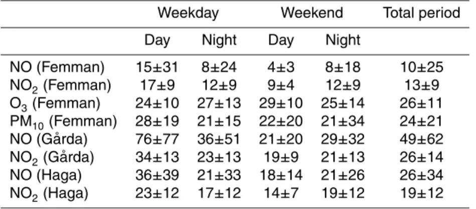
Interactive Discussion Table 3. Mean and standard deviation of NO, NO2, O3(nmol mol−

1

) and PM10(µg m− 3

) during the G ¨ote-2005 campaign (2 February to 2 March) based on measurements at rooftop level in the city centre (Femman), a site close to a traffic route (G ˚arda) and a site in a city street environment (Haga). Daytime is 06:00 to 18:00. Weekdays N=252 (21∗_{12), weekend days}

N=96 (8∗_{12) and total period is N} =696 h.

Weekday Weekend Total period

Day Night Day Night

NO (Femman) 15±31 8±24 4±3 8±18 10±25

NO₂(Femman) 17±9 12±9 9±4 12±9 13±9

O₃(Femman) 24±10 27±13 29±10 25±14 26±11

PM10(Femman) 28±19 21±15 22±20 21±34 24±21

NO (G ˚arda) 76±77 36±51 21±20 29±32 49±62

NO2(G ˚arda) 34±13 23±13 19±9 21±13 26±14

NO (Haga) 36±39 21±33 18±14 21±26 26±34

(24)

ACPD

9, 2081–2111, 2009

J. Klingberg et al.

Title Page

Tables Figures

◭ ◮

Back Close

Full Screen / Esc

0 400 800Meters

1 7

6 5 4 3 2 Göta

Rive r

Haga Gårda

Gothenburg

(25)

ACPD

9, 2081–2111, 2009

J. Klingberg et al.

Title Page

Tables Figures

◭ ◮

Back Close

Full Screen / Esc

02 04 06 08 10 12 14 16 18 20 22 00

0 2000 4000 6000 8000 10000 12000

N

um

ber

of

v

ehic

les

02 04 06 08 10 12 14 16 18 20 22 00

0 0.5 1 1.5 2 2.5

E

m

is

s

io

n

r

a

te

(

g

s

-1 km

-1 )

Time of day

1

Fig. 2. Diurnal variation of vehicle number and emission rate of NOxat Olskroksmotet used in

(26)

ACPD

9, 2081–2111, 2009

J. Klingberg et al.

Title Page

Tables Figures

◭ ◮

Back Close

Full Screen / Esc

0 10 20 30 40 50 60 70 80 90

Haga Gårda Femman 1 2 3 4 5 6 7 8

Site

M

o

le

fr

ac

ti

on

(n

m

o

l m

o

l

-1)

NO NO2 O3

1

(27)

ACPD

9, 2081–2111, 2009

J. Klingberg et al.

Title Page Abstract Introduction Conclusions References Tables Figures ◭ ◮ ◭ ◮ Back Close

Full Screen / Esc

Interactive Discussion 02 04 06 08 10 12 14 16 18 20 22 00

0 50 100

Femman a

02 04 06 08 10 12 14 16 18 20 22 00 0 50 100 Gårda M o le f rac tion ( n m o l m o l -1)

02 04 06 08 10 12 14 16 18 20 22 00 0

50 100

Haga

Time of day

NO NO2

02 04 06 08 10 12 14 16 18 20 22 00 0

50 100

Femman b

02 04 06 08 10 12 14 16 18 20 22 00 0 50 100 Gårda Mo le f ra c tio n ( n mo l mo l -1)

02 04 06 08 10 12 14 16 18 20 22 00 0

50 100

Haga

Time of day

NO NO2

Fig. 4. The average diurnal cycle of NO and NO2 at the urban monitoring sites during the

(28)

ACPD

9, 2081–2111, 2009

J. Klingberg et al.

Title Page Abstract Introduction Conclusions References Tables Figures ◭ ◮ ◭ ◮ Back Close

Full Screen / Esc

Printer-friendly Version Interactive Discussion 0 10 20 30 40 50 60 70 80 90

1 2 3 4 5 6 7 Site NO ( n m o l m o l -1)

TA P M o bs a

y = 0.86x + 13.5 r2_{= 0.49 R}2_{= 0.29} 0 20 40 60 80 100

0 20 40 60 80 1 Modelled O3 (nmol mol-1)

O bs er v ed O 3 ( n m o l m o l -1) 00 Site 1 Site 2 Site 3 Site 4 Site 5 Site 6 Site 7 d 1 0 10 20 30 40 50 60 70 80 90

1 2 3 4 5 6 7 Site NO 2 (n m o l m o l -1)

TA P M o bs b

y = 0.68x + 3.1 r2 _{= 0.51 R}2_{= 0.13} 0 10 20 30 40 50

0 10 20 30 40 5 Modelled NO2 (nmol mol-1)

O bs er v ed N O2 ( n m o l m o l -1) 0 Site 1 Site 2 Site 3 Site 4 Site 5 Site 6 Site 7 e 2 0 10 20 30 40 50 60 70 80 90

1 2 3 4 5 6 7 Site O3 ( n mol mol -1)

TA P M o bs c

y = 0.73x + 5.2 r2 _{= 0.58 R}2_{= 0.44} 0 10 20 30 40 50

0 10 20 30 40 Modelled O3 (nmol mol-1)

O bs er v ed O 3 ( n mo l mo l -1) 50 Site 1 Site 2 Site 3 Site 4 Site 5 Site 6 Site 7 f 3

Fig. 5.Modelled and observed O3, NO2and NO at seven sites during the G ¨ote-2005 period (2

(29)

ACPD

9, 2081–2111, 2009

J. Klingberg et al.

Title Page

Tables Figures

◭ ◮

Back Close

Full Screen / Esc

02 04 06 08 10 12 14 16 18 20 22 00

0 20 40 60 80 100 120

M

o

le f

rac

tion (

n

m

o

l m

o

l

-1 )

Time of day

NO NO₂ O₃

Fig. 6. Diurnal cycle of NO2, NO and O3 concentration at site 6 from 2–27 February 2005

(30)

ACPD

9, 2081–2111, 2009

J. Klingberg et al.

Title Page

Tables Figures

◭ ◮

Back Close

Full Screen / Esc

2 3 4 5 6 7 8

0 0.5 1 1.5 2 2.5 3

Rooftop wind speed (m s-1)

[N

O 2

]s

ite

#

/

[N

O 2

]Fe

m

a

n

Site 7 Site 2 Site 6 Site 5 Site 3 Site 4

Fig. 7. NO2 concentration ratio of sites 2 to 7 and the rooftop monitoring site Femman in

(31)

ACPD

9, 2081–2111, 2009

J. Klingberg et al.

Title Page

Tables Figures

◭ ◮

Back Close

Full Screen / Esc

0.0 0.5 1.0 1.5 2.0 2.5 3.0 3.5

wind 0-1 wind 1-2 wind 2-3 wind 3-4 wind 4-5 wind 5-6 wind 6-7

Modelled wind speed (m s-1)

[NO

2

]site

#

/

[N

O2 ]Femm

an

site7/site1 site2/site1 site3/site1 site4/site1 site5/site1 site6/site1

6 %

4 %

10 % 15 %

22 % 26 %

17 %

Fig. 8. NO2 concentration at site 2 to 7 averaged for different wind speed categories and