www.clim-past.net/3/577/2007/
© Author(s) 2007. This work is licensed under a Creative Commons License.
of the Past
Ice thinning, upstream advection, and non-climatic biases for the
upper 89% of the EDML ice core from a nested model of the
Antarctic ice sheet
P. Huybrechts1,2, O. Rybak2,3, F. Pattyn4, U. Ruth2, and D. Steinhage2
1Departement Geografie, Vrije Universiteit Brussel, Pleinlaan 2, 1050 Brussel, Belgium
2Alfred-Wegener-Institut f¨ur Polar- und Meeresforschung, Postfach 120161, 27515 Bremerhaven, Germany 3Scientific Research Centre, Russian Academy of Sciences, Teatralnaya 8-a, 354000 Sochi, Russia
4Laboratoire de Glaciologie Polaire, D´epartement des Sciences de la Terre et de l’Environnement (DSTE), Universit´e Libre
de Bruxelles, CP160/03, Av. F. Roosevelt 50, 1050 Bruxelles, Belgium Received: 3 April 2007 – Published in Clim. Past Discuss.: 7 May 2007
Revised: 3 September 2007 – Accepted: 11 September 2007 – Published: 2 October 2007
Abstract. A nested ice flow model was developed for east-ern Dronning Maud Land to assist with the dating and inter-pretation of the EDML deep ice core. The model consists of a high-resolution higher-order ice dynamic flow model that was nested into a comprehensive 3-D thermomechani-cal model of the whole Antarctic ice sheet. As the drill site is on a flank position the calculations specifically take into ac-count the effects of horizontal advection as deeper ice in the core originated from higher inland. First the regional veloc-ity field and ice sheet geometry is obtained from a forward experiment over the last 8 glacial cycles. The result is subse-quently employed in a Lagrangian backtracing algorithm to provide particle paths back to their time and place of depo-sition. The procedure directly yields the depth-age distribu-tion, surface conditions at particle origin, and a suite of rel-evant parameters such as initial annual layer thickness. This paper discusses the method and the main results of the ex-periment, including the ice core chronology, the non-climatic corrections needed to extract the climatic part of the signal, and the thinning function. The focus is on the upper 89% of the ice core (appr. 170 kyears) as the dating below that is increasingly less robust owing to the unknown value of the geothermal heat flux. It is found that the temperature biases resulting from variations of surface elevation are up to half of the magnitude of the climatic changes themselves.
Correspondence to:P. Huybrechts ([email protected])
1 Introduction
Physical and chemical properties of Antarctic ice cores con-tain information on past changes of climatic variables such as temperature, atmospheric gas composition, and biogeochem-ical aerosol fluxes reaching back several hundred thousands of years in time. Relevant proxy data have been obtained from long ice cores drilled at the Vostok, Dome Fuji, Dome C, and Kohnen stations (Petit et al., 1999; Watanabe et al., 2003; EPICA community members, 2004, 2006). Drilling of the latter two cores was carried out within the framework of the European Project for Ice Coring in Antarctica (EPICA).
EDC3 time scale was in turn obtained from glaciological modeling at Dome C constrained by well-dated age control points for both cores transferred using the tight stratigraphic link (EPICA community members, 2004, 2006; Ruth et al., 2007; Severi et al., 2007; Parrenin et al., 2007).
The second problem which needs to be addressed results from the dynamics of the Antarctic ice sheet over the time period covered by the ice core. Most importantly, the sur-face elevation at the time of deposition of the ice has varied under the influence of changes in accumulation rate, ice tem-perature, the position of the grounding line, horizontal ice flow, and possibly other factors (Huybrechts, 2002). These elevation changes cause non-climatic biases in the tempera-ture records retrieved from the ice cores. The long isotope records from Dome Fuji and Dome C were acquired from relatively stable ice domes with little or no horizontal move-ment that probably underwent vertical glacial-interglacial elevation changes of the order of 100–200 m (Huybrechts, 2002). With a typical surface temperature lapse rate on the Antarctic plateau of –0.014◦C m−1(Fortuin and Oerlemans, 1990), this corresponds to biases of the order of 2–3◦C, or about 25% of the inferred glacial-interglacial temperature shift. Kohnen station, however, differs from these latter lo-cations as it is not situated on a dome. Instead, it is located along the axis of a gently sloping ridge near to a saddle point about 80 km further downslope. In the upstream direction, the ice divide can be traced for about 1280 km up to Dome Fuji. Because of its flank position, deeper ice at Kohnen was deposited further inland at a progressively higher elevation. This causes an additional non-climatic bias, the strength of which depends on the magnitude of the horizontal velocity and the upstream slope of the ice sheet. For a typical up-stream flow velocity of 1 m yr−1 and an upstream surface gradient of 1.7×10⁻³this corresponds to an additional bias of about 2.5◦C per 100 000 years, which systematic contribu-tion is equally non-negligible compared to the climate signal itself.
Our approach to obtaining the chronology and non-climatic biases is to accurately model the ice sheet history and its flow dynamics for the full time span covered by the ice core. This is done over the entire region where ice particles ending up at Kohnen are believed to have origi-nated. We nested a high-resolution higher-order ice dynamic model, hereafter called FSM (Pattyn, 2003), within a three-dimensional thermomechanically whole Antarctic ice sheet model, hereafter called LSM (Huybrechts, 2002). The re-constructed high-resolution velocity field from a forward ex-periment with the nested model was subsequently used in a Lagrangian backtracing algorithm to establish the trajec-tories of ice particles back to their respective places of de-position. The latter information can be directly linked to a wealth of spatio-temporal parameters required for a correct interpretation of the ice core. The procedure fully accounts for time-dependent changes in such crucial parameters as ice thickness, flow direction, flow velocity, accumulation rate,
and basal melting rates. In contrast to the earlier model study of Savvin et al. (2000) with SICOPOLIS, our model has a much higher resolution as allowed for by detailed observa-tional data from the various EDML pre-site surveys. The nested FSM furthermore includes longitudinal and horizon-tal shear stress gradients in the stress balance, and use was made of Lagrangian backward tracing from the known loca-tion of the ice core site.
The time period under consideration is limited to approx-imately the last 170 kyr. This time span corresponds to the upper 89% or 2477 m of the ice core. It covers all of the last glacial cycle and the previous interglacial, and a signif-icant fraction of the penultimate glacial period. The inter-pretation of the deepest layers increasingly depends on the unknown value of the geothermal heat flux, and the associ-ated rate of basal melting, and was therefore excluded from the present analysis. The models and the Lagrangian back-tracing method are explained in Sects. 2 and 3. It is followed by a discussion of the ice core chronology, the non-climatic biases, and the thinning function in Sects. 4 and 5. Conclu-sions are summarized in Sect. 6.
2 The nested ice sheet model for the forward experi-ment
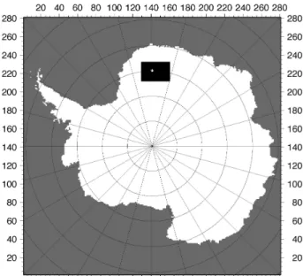
The nested ice sheet model has two components. The Large Scale Model covers all of the Antarctic ice sheet and is run on a 20 km horizontal resolution grid with 30 layers in the verti-cal. It provides boundary conditions for the Fine Scale Model which is implemented over an area of 600 km×400 km in eastern Dronning Maud Land. The FSM grid has a 2.5 km horizontal resolution with 101 equally-spaced layers in the vertical and comprises all of the area where Kohnen ice par-ticles are believed to have originated. All prognostic calcu-lations (ice thickness, bed elevation, ice temperature) take place in the LSM. The main output of the FSM is the diag-nostic three-dimensional velocity field in the nested domain as a function of time. All model parameters employed in FSM correspond to those defined in LSM. The only differ-ence between LSM and FSM concerns the approximations made in the force balance to calculate the horizontal veloc-ity components. Figure 1 shows the respective domains over which both the LSM and FSM are implemented.
2.1 The large scale model LSM
horizontal planes is considered. Longitudinal stress gradients in the flow direction and shear stress gradients perpendicular to the flow are ignored owing to the small height-to-width aspect ratio (Hutter, 1983). LSM accounts for grounding-line migration through explicit modeling of ice shelf flow and a stress transition zone across the grounding line in combi-nation with a floatation criterion. The model is driven by prescribed changes of sea level, surface temperature, surface mass balance and melting below the ice shelves. The en-hancement factor in Glen’s flow law has been slightly read-justed from the earlier value of 2 to a new value of 1.2 to op-timally represent the observed ice thickness in eastern Dron-ning Maud Land in a time dependent run covering the last 8 glacial cycles. In this way, the modeled surface elevation in LSM differs by less than 50 m from the observations over the whole area covered by the FSM domain. Apart from this slight retuning, all other formulations and model param-eters are identical to those given in Huybrechts and de Wolde (1999) and Huybrechts (2002), and are therefore not repeated again. The standard geothermal heat flux of 54.6 m W m−2is applied at the lower boundary of a 4 km thick bedrock slab underlying the ice sheet. The time step for the numerical in-tegration of the continuity equation is 1 year, but larger for numerically more stable quantities such as ice temperature, ice age, and bedrock height.
2.2 The fine scale model FSM
The FSM is a so-called higher-order model as it includes both longitudinal and transverse stress gradients in the force bal-ance equations (Pattyn, 2003). These additional terms im-prove the velocity solution at ice divides, near to the ice-sheet margin, and in areas with pronounced relief or high velocity gradients. They are also required for a more realistic solu-tion on numerical grids where the horizontal resolusolu-tion is of the order of the ice thickness, as is the case here. The solu-tion obtained here is also known as the incomplete 2nd order approximation because vertical pressure is still considered glaciostatic, meaning there are no vertical resistive stresses or bridging effects (Blatter, 1995). Since the horizontal veloci-ties no longer depend on local quantiveloci-ties such as ice thickness and surface slope, as is the case in the shallow-ice approxi-mation, the solution needs to be obtained with iterative meth-ods. The iteration on the nonlinear ice viscosity part is based on a subspace relaxation algorithm, but does not converge very rapidly. Consequently, the FSM is up to 500 times more time consuming than the LSM for a similar grid, and there-fore can only be used for a limited area. Moreover, halving the horizontal grid size in prognostic calculations requires four times more memory and increases CPU time by a factor 16, further limiting the applicability of high-resolution grids to large domains. The vertical velocity field in the nested domain of FSM is obtained through vertical integration of the continuity equation, satisfying kinematic boundary con-ditions at either the upper or lower ice surfaces.
Fig. 1.The Antarctic ice sheet model covers a 281×281 gridpoint square centered over the South Pole. The black rectangle in eastern Dronning Maud Land shows the model domain of the nested re-gional model FSM. The white star denotes the location of Kohnen Station (75◦00.104′S, 0◦04.07′E).
In this study FSM consists only of the higher-order me-chanical equations for the horizontal velocity components as given in Pattyn (2003). The flow law, rheological parameters, and the treatment of basal sliding are identical to LSM. On the 2.5 km grid employed here FSM computes a significantly more accurate velocity field in response to topographic dis-turbances (Hindmarsh et al., 2006). Bedrock perturbations inevitably lead to variations in the flow field. These vari-ations are exaggerated in an SIA model, especially at high resolution where horizontal grid sizes approach the ice thick-ness. This limitation can be overcome by using a coarser grid, but at the expense of a less detailed solution. A higher-order model is insensitive to this effect as long stresses de-velop where gradients are more pronounced, in effect smear-ing out the effects of small-scale irregularities (Pattyn et al., 2005). Without FSM we could therefore not have exploited the quality of the detailed observations to the same extent. This is best illustrated by the resulting ice core chronologies, which differed by up to 20% at 90% depth between FSM and LSM as obtained from their velocity solutions on their respective grids.
2.3 Geometric model input and coupling scheme
Fig. 2.Fundamental model input on the 2.5 km grid of the FSM. Left panel: bedrock elevation in m a.s.l.; right panel: present-day accumu-lation rate in m yr−1of ice equivalent. These datasets are a combination of the BEDMAP data and the earlier compilations of Huybrechts et al. (2000) updated with the results of extensive pre-site field surveys conducted by the Alfred Wegener Institute. The integer coordinates of the FSM domain correspond to the 20 km gridpoints of the LSM.
(Steinhage et al., 2001) and blended with the older datasets for oceanic bathymetry (Huybrechts et al., 2000) to circum-vent artefacts in the BEDMAP data at grounding lines and below ice shelves. The bedrock topography in the domain covered by FSM includes the most complete collection of radio-echo-sounding flight lines as obtained by the Alfred Wegener Institute. The flight line separation over the en-tire area where particle trajectories are located is better than 10 km with crossover differences in ice thickness less than 10 m for the majority of cases. Near to Kohnen station the radar profile separation densifies to less than 1 km due to the radial flight pattern, justifying the 2.5 km grid resolution em-ployed in FSM. For surface elevation, the 2.5 km grid is a high-resolution cubic-spline representation of the 20 km grid, in effect causing surface gradients in FSM to represent av-erage values over a distance of about 10 ice thicknesses as dictated by theory (Paterson, 1994). For ice thickness and bedrock elevation, on the other hand, overlapping gridpoints of FSM and LSM do not have exactly the same values. Fig-ure 2 (left panel) shows the bedrock topography in the nested model domain.
The field of accumulation rate is based on the Giovinetto and Zwally (2000) compilation used in Huybrechts et al. (2000), and updated with accumulation rates obtained from shallow ice cores during the EPICA pre-site surveys (Oerter et al., 1999, 2000; Rotschky et al., 2007). The present-day accumulation rate at Kohnen in this dataset is 7.0 cm yr−1of ice equivalent (Fig. 2, right panel).
The coupling between FSM and LSM is performed in a straightforward manner. LSM exchanges information with FSM only in the downward direction; the high-resolution flow solution does not feed back into the Large Scale Model. All information is passed down using cubic-splines as inter-polation algorithm (Press et al., 1992). We experimented with two anomaly schemes to transfer changes in geomet-ric variables (surface elevation, ice thickness, and bed ele-vation). In the first one anomalies, or differences, of LSM variables at time t with respect to the observations are
Fig. 3. Modeled present-day horizontal surface velocity (m yr−1) as obtained by the FSM. The modeled value for Kohnen Station of 0.73 m yr−1is very close to the observed value of 0.76 m yr−1. Meridians and parallel circles are both plotted at a 1◦spacing.
The present-day modeled field of horizontal surface veloc-ity in FSM is displayed in Fig. 3. Kohnen station is shown to be located almost exactly on the flow axis with horizon-tal velocities decreasing downstream when approaching the saddle area. The modeled surface velocity at Kohnen is 0.73 m yr−1, close to the currently observed surface
veloc-ity of 0.76 m yr−1(Wesche et al., 2007). The corresponding
vertically averaged velocity is 0.65 m yr−1from a direction
close to westward (279.4◦ azimuth in the model compared to 273.4◦ observed). The model predicts no basal sliding at Kohnen at present concomitant with a basal temperature 0.3◦C below the pressure melting point. However, as the EDML drill site is located very close to the melting point and is adjacent to a large wet-based zone further to the south, the pressure melting point was hit intermittently on many oc-casions during the last few glacial cycles. As present-day melting already occurs for a slightly higher geothermal heat flux of 56 m W m−2, well within the uncertainty range on this
parameter (Fox Maule et al., 2005), the exact history of basal melting at Kohnen is hard to predict. We therefore restrict the analysis of the EDML ice core to the uppermost 89% which are largely unaffected by the unknown basal boundary con-dition on temperature and velocity. Field evidence from the drilling itself found subglacial water entering the borehole, indicating pressure melting conditions also today, and conse-quently, a geothermal heat flux at least 1.4 m W m−2higher than assumed by the standard model.
2.4 Experimental set-up
The nested model was first integrated over the last 740 kyr. This is the period coinciding with the last 8 glacial cycles for which detailed climatic forcing from both Antarctic ice cores and oceanic sediment cores is available. The sea level forc-ing, which controls grounding-line migration in LSM, was
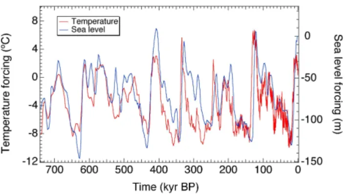
Fig. 4. Climatic forcing records used in the forward experiment over the last 8 glacial cycles. The temperature forcing was assem-bled from a combined EDC/EDML isotope record subject to surface elevation corrections from a precursor experiment. The sea level forcing record was assembled from the Bassinot and SPECMAP oceanicδ18O stacks.
put together by combining a planktonicδ18O record from the tropical ocean (Bassinot et al., 1994) with the well-known SPECMAP stack (Imbrie et al., 1984). Both were scaled to obtain a sea-level minimum of –130 m at the Last Glacial Maximum and a sea-level maximum of +6 m during the Last Interglacial around 122 kyr BP (Chappell and Shackleton, 1986). We took the Bassinot record because its chronol-ogy already served to construct age control windows for the dating of the EDC ice core for the period older than 50 ky BP (EPICA community members, 2004). The SPECMAP data provides the sea-level forcing only for the most re-cent 21 kyr following the Last Glacial Maximum when the Bassinot record is incomplete.
For the temperature forcing, we made use of both the EDC deuterium record (EPICA community members, 2004) for the last 740 kyr and the EDMLδ18O record for the last 170 kyr (EPICA community members, 2006). These were provided on early 2006 draft versions of the EDML1 and EDC3 time scales, virtually identical to their final forms (Ruth et al., 2007 issue; Parrenin et al., 2007). The correction for the mean isotopic content of the ocean was made follow-ing Vimeux et al. (2002) employfollow-ing the Bassinot et al. (1994)
1δ18Ooceanscaled for a global meanδ18O enrichment of 1‰
at the LGM (Waelbroeck et al., 2002). An iterative proce-dure was adopted to estimate the climatic part of the ice core signals. First, LSM was run over 740 000 years using the EDC deuterium record with∂Ts/∂δD=0.166◦C/‰. Modeled
forcing records obtained in this way are displayed in Fig. 4. The nested LSM/FSM experiment described in this paper in fact represents one more iteration to obtain the ice core cor-rections using those pre-determined forcing functions. The local accumulation rate in the large ice sheet and the nested flow model is calculated from the thermodynamical depen-dence of precipitation rate on the temperature at the eleva-tion of cloud formaeleva-tion over the ice sheet (Jouzel and Mer-livat, 1984), using a modification of the Lorius et al. (1985) approach (EPICA community members, 2004):
PA[TI(t )]=PA[TI(0)] exp
22.47
T
0
TI(0)
− T0
TI(t )
T
I(0)
TI(t )
2
{1+β[TI(t )−TI(0)]} (1)
where PA[TI(t )] is the local accumulation rate at time t,
PA[TI(0)] the present-day accumulation rate at the same
place,T0 =273.15 K,TI(t )= 0.67TS(t )+88.9 (in K) is
the inversion temperature at time t andTI(0)is the
present-day inversion temperature. β is a constant fitting parame-ter. The first part of the relation basically takes into account the temperature-dependent change of saturation vapour pres-sure, whereas the parameter β takes into account glacial-interglacial changes of the accumulation pattern that is not explained by this relationship.β=0.046 has been empirically determined by comparing upstream accumulation rates de-rived from firn cores (Oerter et al., 2000; Graf et al., 2002) with the internal layering from an extended surface radar sur-vey along the Kohnen-Dome Fuji radio-echo sounding pro-file (Steinhage et al., 2001; Rybak et al., 2005). This leads to average glacial accumulation rates around the EDML drill site which are around 45% of current values. The approach assumes that the current spatial pattern of accumulation rate is conserved through time and that spatially-derived temper-ature lapse rates are invariant in time.
3 Backward tracing of particle trajectories
3.1 Lagrangian backtracing method
The forward experiment stores the three-dimensional veloc-ity field, ice thickness, surface elevation, surface tempera-ture, accumulation rate, and other relevant variables for every 100 years in a FSM subdomain that is large enough to em-bed all possible trajectories. Initially, ice particles are placed at every 0.1% of ice equivalent thickness (or every 2.75 m) at the exact geographical position of the Kohnen drill site. Each particle is then rigorously traced back into time along La-grangian particle paths using the inverse three-dimensional velocity field interpolated by three-dimensional splines to the exact particle position. This is equivalent to the Particle-in-Cell method (Harlow, 1964) and the reverse of the method qualitatively described in Reeh (1989) for reconstructing for-ward particle paths or the method to determine isochrones in
numerical ice sheet models (Rybak and Huybrechts, 2003). The timetwhen the ice particle crosses the ice sheet surface is accepted as the time of origin, or age, of the ice, and the x,y-coordinates of surface emergence as the place of origin, which information can be further linked to a number of rel-evant variables. To improve the dating, an algorithm is used to calculate the exact age within a fraction of the time step
1t=100 years by estimating the time left to reach the surface by the tracer already closest to the surface.
3.2 Particle trajectories and points of origin
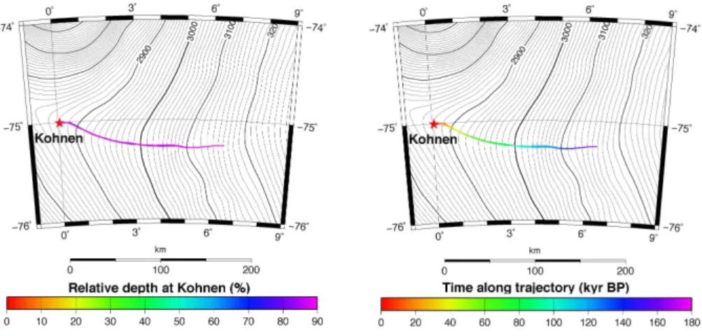
The left panel of Fig. 5 shows the horizontal projections of all particle trajectories for the upper 89% of the EDML ice core, plotted on a background representing the present-day observed topography. The deepest particle traveled for 184 km roughly parallel to a latitudinal circle. Only the deepest particle trajectories are visible on the plot in purple colours, attesting to the stability of the flow pattern and the ice di-vide position in this region over the time period considered. Apparently all these trajectories followed almost the same path with a maximum bandwidth of less than 2 km. The right panel of Fig. 5 shows the same particle trajectories, but now coloured as a function of time. The gradual change of colours again attests to the relatively constant flow magnitude along the ridge which varied around 1 m yr−1for most of the tra-jectories during the last 170 kyr.
The points of origin where Kohnen particles were origi-nally deposited is displayed in Fig. 6 as a function of EDML depth and time of deposition. It is found that the deepest par-ticle ending up at 89% relative depth was deposited 169.9 kyr ago at the ice sheet’s surface. As the time of deposition is equivalent to the age of a particle, these results immediately yield the chronology of Kohnen ice.
3.3 Ice core chronology
Fig. 5.Horizontal projection of ice particle trajectories placed at every 1% i.e. depth in the Kohnen drill site. The colour coding in the left panel is for their final depth at Kohnen. In the right panel the colours indicate the time along any individual trajectory. Since most trajectories follow similar paths, the younger ones are overlain by the deepest particle trajectories which travelled furthest. The background contour lines are for the present-day surface elevation. Results are only shown for the uppermost 89% of the ice core.
Fig. 6.Places of origin for particles placed at every 1% i.e. depth in the Kohnen drill site. These are shown as a function of relative depth at Kohnen (left panel) and time of deposition (right panel). The background contour lines are for the present-day surface elevation. Results are only shown for the uppermost 89% or 169 kyr of the ice core.
to glacial-interglacial shifts in accumulation rate, and hence, initial ice layer thickness at the surface.
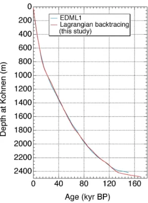
Comparing our glaciologically derived chronology with EDML1 shows an excellent agreement for most of the pro-file. This proves the validity and internal consistency of the modeled velocity fields and gives confidence in our parti-cle trajectory method. The agreement is very good for the Holocene and long time intervals during the last glacial pe-riod with a maximum age difference of less than 300 years. Somewhat larger differences are seen for several segments below 1000 m depth of up to 1750 yr at 1760 m and at 2110 m depth. The most conspicuous deviation from EDML1 how-ever takes place for the bottom part of the comparison below 2380 m (ice older than 130 kyr) where EDML1 gives consid-erably older ages than our modelling. The reasons for these mismatches are however unclear, in particular as they do not
Fig. 7. Model-derived depth-age distribution at Kohnen plotted as function of real depth. For comparison, the EDML1 time scale ob-tained from stratigraphic matching with the EDC ice core is shown in blue (Ruth et al., this issue). Both curves agree very well, but less so for the penultimate glacial period between 125 and 150 kyr BP.
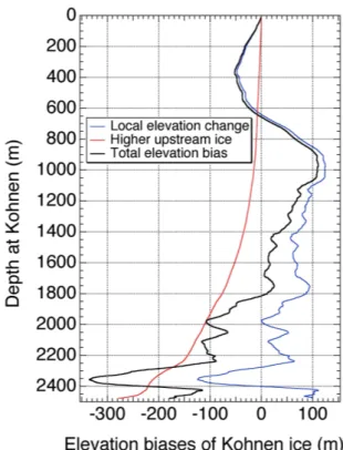
Fig. 8.Differences in surface elevation (m) of Kohnen ice with re-spect to its present-day elevation shown as a function of time. The total elevation bias (black line) has a component due to horizon-tal advection (red line, given as the elevation difference between Kohnen and the place of origin of the ice particle for present-day topography) and due to the local elevation change at the point of particle origin at the time of deposition (blue line, given as the ele-vation difference at the place of origin between today and the time of origin).
thinning function, but a definite proof of their occurrence at this depth has yet to be given. Unless the mismatches are caused by model errors or other physical mechanisms we are unaware of, it is also possible that the stratigraphic matching and/or the EDC3 chronology are imprecise. That may espe-cially be the case for the bottom part below 2350 m where confidence in the synchronization method is lower (Ruth et al., 2007); however, investigations have shown that possi-ble stratigraphic mismatches could only account for part of the observed deviations. Therefore it seems likely that the mismatches between the purely glaciologically derived time scale and EDML1 is some combination of all the factors mentioned above. We can probably exclude the role of possi-ble basal melting upstream of the Kohnen drill site, because any basal melting would have made the modelled ice even younger as compared to EDML1, and our standard model predicts continuously frozen conditions. Finally, it is inter-esting to note that tentative extensions of both chronologies not shown here seem to match up again around 180 ky.
4 Non-climatic biases
Since ice particles have recorded physical conditions at the time and place of origin, it is clear from the preceding dis-cussion that this information is contaminated by elevation changes. Any climatic interpretation of ice core variables therefore needs to be corrected for these elevation changes. The older the ice at Kohnen, the further upstream it was de-posited. Since particle trajectories approximately followed a circle of latitude, we can neglect latitudinal climatic gra-dients. We define non-climatic biases as a function of the elevation difference between the original altitude at particle deposition and the present-day altitude of Kohnen. A distinc-tion is made between a bias due to advecdistinc-tion1Sadvand one
due to the local elevation change1Sloc:
1Sadv(t )=SEDML(0)−Sxy(0) (2)
1Sloc(t )=Sxy(0)−Sxy(t ) (3)
1Stot(t )=1Sadv(t )+1Sloc(t ) (4)
where1Stotis the total elevation bias and the subscriptsxy
and EDML refer to the place of deposition and the current location of the EDML ice core, respectively.
These elevation biases are shown in Fig. 8 as a function of time. The advection bias from the higher upstream ice shows up as a systematic decline modulated by both surface slope and horizontal speed of advection. For the time span considered here, 1Sadv equals –275 m by 170 kyr BP.
Su-perimposed on this systematic trend are the effects of local elevation changes. These are primarily driven by accumula-tion changes, on which the effects of deeper ice temperature and to a lesser extent, grounding line changes at the coast, are superimposed. The local elevation bias1Slochas a
in this part of Dronning Maud Land. It is positive during glacial periods commensurate with the lower accumulation rates, and hence, lower elevations. At present, the surface at Kohnen is lowering at a rate of 8.7 m kyr−1, correspond-ing to a combination of slightly lower accumulation rates since the mid-Holocene, slight warming in the basal defor-mational layers, and the effects of a thinning wave originat-ing from groundoriginat-ing-line retreat after the Last Glacial Max-imum. These responses are very similar to those discussed in Huybrechts (2002). Because of the damming effect of the Maudheimvidda mountain range on the flow, grounding-line changes in both East and West Antarctica exert only a rela-tively minor influence on this part of Dronning Maud Land. As the effect of accumulation is dominant, elevation changes along the flowlines mainly scale with the local accumulation rate compared to Kohnen, and are moreover approximately synchronous with Kohnen. The local elevation bias is domi-nant for the upper half of the ice core but below that the up-stream advection bias is most important. The maximum total elevation bias1Stotof –335 m relative to present-day occurs
during the Last Interglacial at 125.2 kyr BP when accumu-lation rates were highest and the ice was deposited about 150 km inland at a current elevation 220 m higher than to-day. In Fig. 9 the same non-climatic biases are plotted as a function of depth at Kohnen using the modeled age to depth time scale.
To transform these elevation biases into temperature and
δ18O corrections present-day spatial correlations between 10-m firn temperature, surface elevation, and mean surface
δ18O need to be established. This was done using a sub-set of the pre-site survey data located upstream from Kohnen (Oerter et al., 1999, 2000; Graf et al., 2002). The linear re-lations resulting from this regression are shown in Fig. 10. Consequently, non-climatic biases on surface temperature andδ18O are found as:
btotT (t )=bTadv(t )+bTloc(t )=1Sadv(t )
∂TS
∂S +1Sloc(t ) ∂TS
∂S (5)
btotδ18O(t )=bδadv18O(t )+blocδ18O(t )=1Sadv(t )
∂δ18O ∂S
+1Sloc(t )
∂δ18O
∂S (6)
where b is the non-climatic bias and∂TS∂S= –0.01171◦C
m−1and∂δ18O
∂S= –0.00957‰ m−1. The usual assump-tion is made that present-day spatial gradients are a good approximation for temporal gradients (Jouzel et al., 1997). This need not necessarily be the case. For example, Krinner and Genthon (1999) established from numerical experiments with AGCMs that the temporal Antarctic lapse rate at 3000 m elevation may be somewhat lower at∂Ts∂S= –0.009◦C
m−1. If so, our non-climatic temperature bias may be over-estimated by about 25%.
Fig. 9.Same biases as in Fig. 8 but plotted as a function of depth at Kohnen using the modeled depth-age distribution.
Final non-climatic corrections for surface temperature and
δ18O are shown in Fig. 11 as a function of time. These are the values which need to be added to the measured δ18O ratios obtained directly from the EDML ice core. Appar-ently, the LGM was about 1◦C cooler and MIS 5.5 up to 4◦C warmer than evident from the uncorrected ice core data themselves because of the elevation biases. These correc-tions amount to about half of the range of the original data for the older ice analysed in this paper, which is certainly not negligible. The elevation biases are generally also of larger magnitude than the oceanic correction required to ac-count for changes in the mean δ18O composition of the oceans (EPICA community members, 2006). A complete list of the non-climatic biases is also given in the supplemen-tary Tables S1 and S2 (http://www.clim-past.net/3/577/2007/ cp-3-577-2007-supplement.zip).
5 Thinning function
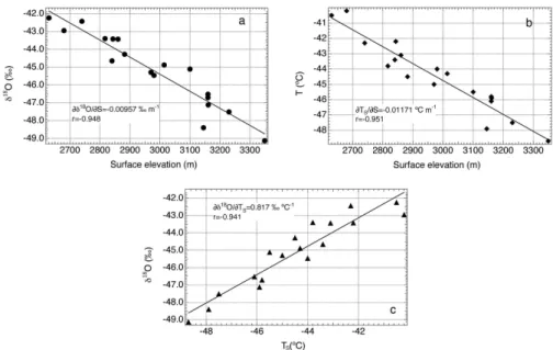
Fig. 10.Linear regression relations between present-day surface elevation (S, in m), surface temperature (Ts, in◦C) and oxygen-isotope value
of surface snow (δ18O, in ‰) for a selection of field sites upstream of the Kohnen drill site (Oerter et al., 1999, 2000). The calculated present-day spatial gradients are used to transform the modeled elevation changes into non-climatic biases and to correct the initial temperature forcing record. The high values of the correlation coefficients r attest as to the validity of the linear relationships.
Fig. 11.Total non-climatic biases for the last 169 kyr in the EDML ice core displayed both as a function of surface air temperature (◦C, left axis) and ofδ18O value (‰, right axis) using the linear relations shown in Figure 10.
λ(z), ice age A(z), accumulation ratePA(z), and thinning
functionR(z), e.g. Reeh (1989), Parrenin et al. (2004):
A (z)=
z
Z
0
dz′ PA(z′) R (z′)
(7)
R(z)= λ(z)
λ0
(8) whereλ0=PA(t )is the initial annual layer thickness at the
surface.
In our calculations the strain thinning function was rigor-ously derived from tracing back the layer thickness at a
cer-tain depth in the ice core to the original accumulation rate at the surface over exactly the same time interval. This required taking much smaller time steps in the Lagrangian backtrac-ing algorithm than the standard 100 years for the last 50 kyr. Additionally, a correction was made for firn compaction in the upper 180 m by fitting a relation for firn density ρ (z)
to the observed density profile of the B32 core (Oerter and Wilhelms, 2001) obtained by dielectric profiling (Wilhelms, 2005):
ρ (z)=ρ0−(ρ0−ρsur+ρc)exp(az)+ρc (9)
where ρ0=910 kg m−3 the density of ice, ρsur=350 kg m−3
snow density at the surface, a=–0.0212 m−1, and
ρc=12.329 kg m−3 a fitting constant to obtain a smooth
density transition at 180 m real depth. The depthzis taken positive downwards.
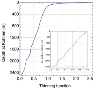
Fig. 12.Thinning function at Kohnen plotted as a function of depth. The blue line is plotted versus real depth and was corrected for a variable firn density in the upper 180 m. The inset shows the origi-nal thinning function obtained in the experiment as a function of ice equivalent depth.
“anomalously high” values for the thinning function between 1600 and 1720 m depth were caused by bedrock highs at around 60 km upstream from Kohnen station as these are the only irregular features corresponding to the approximate time and place of deposition at this depth in the core. Note, however, that the wiggle in the thinning function between 1600 and 1720 m depth is not correlated with any of the mis-matches between our modeled time scale and EDML1 as the age mismatches occur at depths where the thinning function shows no obvious features.
6 Conclusions
In this paper a novel method was presented to date the EDML ice core and separate its climatic information from topo-graphic effects. The main strength of the method is that it is self-contained and largely independent from the specific palaeo-climatic information retrieved from the ice core. The Lagrangian backtracing method in a nested model could as well have been successfully applied to a virtual location else-where on the Antarctic plateau without the need of a priori information about past climatic conditions in that particu-lar site provided geometric boundary conditions such as ice thickness are sufficiently well known.
The general good agreement between our glaciologically derived time scale and the official EDML1 time scale pro-vides a good validation of the models and the method, and therefore lends credibility to apply the method also at other (virtual) sites. It was demonstrated that because of its flank position, deeper ice at Kohnen progressively recorded
cli-mate from higher upstream positions increasingly less rep-resentative for the current drill site. Non-climatic tempera-ture biases from variations of surface elevation were found to amount to up to half of the climate changes retrieved from the ice core itself for the Last Interglacial period. Since the thinning function depends primarily on ice dynamics, any discrepancy between the model-derived age-depth dis-tribution and the one derived from another dating technique should preferentially be interpreted in terms of anomalous accumulation rates, provided substantial changes in ice rhe-ology along the vertical can be excluded.
Sensitivity tests not discussed further in this paper brought to light that the elevation changes and upstream flow cor-rections are robust to our most important model parameters, at least for the upper∼90% of the EDML ice core. Below that, the model chronology and derived characteristics are affected much more by the uncertainties on the basal bound-ary condition, especially on the unknown amount of basal melting. Extending the analysis to these basal layers will re-quire additional efforts to account for the potential range on the geothermal heat flux one could reasonably expect in this part of Dronning Maud Land. The age of the basal ice and the horizontal distance it travelled is moreover expected to increasingly depend on possible ice flow anomalies result-ing from fabric evolution or other deformational defects. A clear and unique solution to the age of the bottom ice may therefore be difficult to obtain from straightforward modeling alone, requiring additional constraints from detailed analyses of the ice core itself.
Acknowledgements. The authors wish to thank K. Ketelsen (DKRZ) for essential help to adapt the model code for parallel computing and S. Frickenhaus (AWI) for fruitful discussions concerning performance of the numerical experiments in the early stage of the research. Discussions with C. Ritz and F. Parrenin (LGGE) as well as with F. Wilhelms (AWI) were also greatly appreciated, as were thoughtful reviewer comments from R. Hind-marsh, an anonymous referee, and the editor. Part of the work was supported by the Belgian Research Programmes on the Antarctic and on Science for a Sustainable Development (Belgian Federal Science Policy Office) under contracts EV/11/08A (AMICS) and SD/CA/02A (ASPI). This work is a contribution to the European Project for Ice Coring in Antarctica (EPICA), a joint European Science Foundation/European Commission scientific programme, funded by the EU (EPICA-MIS) and by national contributions from Belgium, Denmark, France, Germany, Italy, the Netherlands, Norway, Sweden, Switzerland and the United Kingdom. The main logistic support was provided by IPEV and PNRA (at Dome C) and AWI (at Dronning Maud Land). This is EPICA publication no. 178.
References
Bassinot, F. C., Labeyerie, L. D., Vincent, E., Quidelleur, X., Shakelton, N. J., and Lancelot, Y.: The astronomical theory of climate and the age of the Brunhes-Matuyama magnetic rever-sal, Earth Planet. Sci. Lett., 126, 91–108, 1994.
Blatter, H.: Velocity and stress fields in grounded glaciers: a simple algorithm for including deviatoric stress gradients, J. Glaciol., 41(138), 333–344, 1995.
Chappell, J. and Shackleton, N. J.: Oxygen isotopes and sea level, Nature, 324, 137–140, 1986.
EPICA community members: Eight glacial cycles from an Antarc-tic ice core, Nature, 429, 623–628, 2004.
EPICA community members: One-to-one interhemispheric cou-pling of polar climate variability during the last glacial, Nature, 444, 19-5-198, 2006.
Fortuin, J. P. F. and Oerlemans, J.: Parameterisation of the an-nual surface temperature and mass balance of Antarctica, Ann. Glaciol., 14, 78–84, 1990.
Fox Maule, C., Purucker, M. E., Olsen, N., and Mosegaard, K.: Heat Flux Anomalies in Antarctica Revealed by Satellite Mag-netic Data, Science 309, 464–467, 2005.
Giovinetto, M. B. and Zwally, H. J.: Spatial distribution of net sur-face accumulation on the Antarctic ice sheet, Ann. Glaciol., 31, 171–178, 2000.
Graf, W., Oerter, H., Reinwarth, O., Stichler, W., Wilhelms, F., Miller, H., and Mulvaney, R.: Stable-isotope records from Dron-ning Maud Land, Antarctica, Ann. Glaciol., 35, 195–201, 2002. Harlow, F. H.: The particle-in-cell computing method for fluid
dy-namics, Methods of Computational Physics, 3, 319–343, 1964. Hindmarsh, R. C. A., Leysinger Vieli, G. J.-M. C., Raymond,
M. J., and Gudmundsson, G. H.: Draping or Overriding: The Effect of Horizontal Stress Gradients on Internal Layer Architecture in Ice-Sheets, J. Geophys. Res., 111, F02018, doi:10.1029/2005JF000309, 2006.
Hutter, K.: Theoretical Glaciology: material science of ice and the mechanics of glaciers and ice sheets, D. Reidel Publishing Co, Dordrecht etc, 1983, 510 p.
Huybrechts, P.: Sea-level changes at the LGM from ice-dynamic reconstructions of the Greenland and Antarctic ice sheets during the glacial cycles, Quat. Sci. Rev., 21, 203–231, 2002.
Huybrechts, P. and de Wolde, J.: The Dynamic Response of the Greenland and Antarctic Ice Sheets to Multiple-Century Climatic Warming, J. Climate, 12, 2169–2188, 1999.
Huybrechts, P., Steinhage, D., Wilhelms, F., and Bamber, J. L.: Bal-ance velocities and measured properties of the Antarctic ice sheet from a new compilation of gridded data sets for modeling, Ann. Glaciol., 30, 52–60, 2000.
Imbrie, J.Z., Hays, J.D., Martinson, D.G., MacIntyre, A., Mix, A.C., Morley, J.J., Pisias, N.G., Prell, W.L., Shackleton, N.J.: The orbital theory of Pleistocene climate: support from a revised chronology of the marineδ18O record, in: Milankovitch and Cli-mate, edited by: Berger, A., Imbrie, J. Z., Hays, J. D., Kukla, G., and Saltzman, B., 269–305, D. Reidel, Dordrecht., 1984. Jouzel, J. and Merlivat, L.: Deuterium and oxygen 18 in
precipita-tion: modelling of the isotopic effects during snow formation, J. Geophys. Res., 89(D7), 11 749–11 757, 1984.
Jouzel, J., Alley, R. B., Cuffey, K. M., Dansgaard, W., Grootes, P., Hoffmann, G., Johnsen, S. J., Koster, R. D., Peel, D., Shuman, C. A., Stievenard, M., Stuiver, M., and White, J.: Validity of the
temperature reconstructions from water isotopes in ice cores, J. Geophys. Res, 102(C12), 26 471–26 487, 1997.
Krinner, G. and Genthon, C.: Altitude dependence of the ice-sheet surface climate, Geophys. Res. Let., 26, 2227–2230, 1999. Lorius, C., Jouzel, J., Ritz, C., Merlivat, L., Barkov, N. I.,
Korotke-vich, Y. S., and Kotlyakov, V. M.: A 150 000-year climatic record from Antarctic ice, Nature, 316, 591–596, 1985.
Lythe, M., Vaughan, D. G., and the BEDMAP Consortium: BEDMAP: a new ice thickness and subglacial topographic model of Antarctica, J. Geophys. Res., 106(B6), 11 335–11 352, 2001. Oerter, H., Graf, W., Wilhelms, F., Minikin, A., and Miller, H.:
Accumulation studies on Amundsenisen, Dronning Maud Land, Antarctica, by means of tritium, dielectric profiling and stable-isotope measurements: first results from the 1995-96 and 1996-97 field seasons, Ann. Glaciol., 29, 1–9, 1999.
Oerter, H., Wilhelms, F., Jung-Rothenh¨ausler, F., G¨oktas, F., Miller, H., Graf, W., and Sommer, S.: Accumulation rates in Dronning Maud Land, Antarctica, as revealed by dielectric-profiling mea-surements of shallow firn cores, Ann. Glaciol., 30, 27–34, 2000. Oerter, H. and Wilhelms, F.: Physical properties of firn core DML05C98 32 (B32), PANGAEA, doi:10.1594/PANGAEA.58815, 2001.
Parrenin, F., R´emy, F., Ritz, C., Siegert, M. J., and Jouzel, J.: New modeling of the Vostok ice flow line and implication for the glaciological chronology of the Vostok ice core, J. Geophys. Res., 109(D20), D20102, doi:10.1029/2004JD004561, 2004. Parrenin, F., Hindmarsh, R. C. A., and R´emy, F: Analytical
solu-tions for the effect of topography, accumulation rate variasolu-tions and flow divergence on isochrone layer geometry, J. Glaciol., 52(177), 191–202, 2006.
Parrenin, F., Barnola, J.-M., Beer, J., Blunier, T., Castellano, E., Chappellaz, J., Dreyfus, G., Fischer, H., Fujita, S., Jouzel, J., Kawamura, K., Lemieux-Dudon, B., Loulergue, L., Masson-Delmotte, V., Narcisi, B., Petit, J.-R., Raisbeck, G., Raynaud, D., Ruth, U., Schwander, J., Severi, M., Spahni, R., Steffensen, J. P., Svensson, A., Udisti, R., Waelbroeck, C., and Wolff, E.: The EDC3 chronology for the EPICA Dome C ice core, Climate of the Past, 3, 485–497, 2007.
Paterson, W. S. B.: The physics of glaciers, 3rdedition, Elsevier, Oxford, New York, Tokyo, 1994, 480 p.
Pattyn, F.: A new three-dimensional higher-order thermomechani-cal ice sheet model: Basic sensitivity, ice stream development, and ice flow across subglacial lakes, J. Geophys. Res., 108(B8), 2382, doi:10.1029/2002JB002329, 2003.
Pattyn, F., Nolan, M., Rabus, B., and Takahashi, S.: Localized basal motion of a polythermal Arctic glacier: McCall Glacier, Alaska, USA, Ann. Glaciol., 40, 47–51, 2005.
Petit, J. R., Jouzel, J., Raynaud, D., Barkov, N. I., Barnola, J.-M., Basile, I., Bender, M., Chapellaz, J. Davis, M. E., Delaygue, G., Delmotte, M., Kotlyakov, V. M., Legrand, M., Lipenkov, V. Y., Lorius, C., Pepin, L., Ritz, C., Saltzman, E., Stievenard, M.: Cli-mate and atmospheric history of the past 420 000 years from the Vostok ice core, Antarctica, Nature, 399, 429–436, 1999. Press, W. H., Teukolsky, S. A., Vetterling, W. T., and Flannery, B. P.:
Numerical Recipes, 2nd ed., Cambridge University Press, Cam-bridge, 1992, 963 p.
C., J. Wiley & Sons, Chichester, 141–159, 1989.
Rotschky, G., Holmlund, P., Isaakson, E., Mulvaney, R., Oerter, H., Van den Broeke, M., and Winther, J.-G.: A new surface accumu-lation map for western Dronning Maud Land, Antarctica, from interpolation of point measurements, J. Glaciol., 53(182), 385– 398, 2007.
Ruth, U., Barnola, J.-M., Beer, J., Bigler, M., Blunier, T., Castel-lano, E., Fischer, H., Fundel, F., Huybrechts, P., Kaufmann, P., Kipfstuhl, S., Lambrecht, A., Morganti, A., Oerter, H., Parrenin, F., Rybak, O., Severi, M., Udisti, R., Wilhelms, F., and Wolff, E.: “EDML1”: a chronology for the EPICA deep ice core from Dronning Maud Land, Antarctica, over the last 150 000 years, Clim. Past, 3, 475–484, 2007,
http://www.clim-past.net/3/475/2007/.
Rybak, O. and Huybrechts, P.: A comparison of Eulerian and La-grangian methods for dating in numerical ice-sheet models, Ann. Glaciol., 37, 150–158, 2003.
Rybak, O., Huybrechts, P., Steinhage, D., and Pattyn F.: Dating and accumulation rate reconstruction along the Dome Fuji-Kohnen radio echo-sounding profile, Geophys. Res. Abstr., 7, 2005. Savvin, A., Greve, R., Calov, R., M¨ugge, B., and Hutter, K.:
Simulation of the Antarctic ice sheet with a three-dimensional polythermal ice-sheet model, in support of the EPICA project. II: Nested high-resolution treatment of Dronning Maud Land, Antarctica, Ann. Glaciol., 30, 69–75, 2006.
Severi, M., Becagli, S., Castellano, E., Morganti, A., Traversi, R., Udisti, R., Ruth, U., Fischer, H., Huybrechts, P., Wolff, E., Par-renin, F., Kaufmann, P., Lambert, F., and Steffensen, J. P.: Syn-chronisation of the EDML and EDC ice cores for the last 52 kyr by volcanic signature matching, Clim. Past, 3, 367–374, 2007, http://www.clim-past.net/3/367/2007/.
Steinhage, D., Nixdorf, U., Meyer, U., and Miller, H.: Subglacial topography and internal structure of central and western Dron-ning Maud Land, Antarctica, determined from airborne radio echo sounding, J. Appl. Geophys., 47, 183–189, 2001.
Vimeux, F., Cuffey, K. M., and Jouzel., J.: New insights into South-ern Hemisphere temperature changes from Vostok ice cores us-ing deuterium excess correction, Earth. Planet. Sci. Lett., 203, 829–843, 2002
Waelbroeck, C., Labeyrie, L., Michel, E., Duplessy, J. C., Mc-Manus, J. F., Lambeck, K., Balbon, E., and Labracherie, M.: Sea-level and deep water temperature changes derived from ben-thic foraminifera isotopic records, Quat. Sci. Rev., 21, 295–305, 2002.
Watanabe, O., Jouzel, J., Johnsen, S. J., Parrenin, F., Shoji, H., and Yoshida, N.: Homogenous climate variability across East Antarctica over the past three glacial cycles, Nature, 422, 509– 512, 2003.
Wesche, C., Eisen, O., Oerter, H., Schulte, D., and Steinhage, D.: Surface topography and ice flow in the vicinity of EDML deep-drilling site, J. Glaciol., 53(182), 442–448, 2007.