Abstract
This work deals with the design of a suspension device, idealized as a spring-mass-damper system. The amplitude of a nominal system is constrained to satisfy certain limitations in a given frequency band and the design is to be done as a reliability-based optimiza-tion. This constitutes a major difficulty since the constraint becomes a random process. To concentrate in the main ideas, only the stiff-ness of the system will be considered random. The stiffstiff-ness is char-acterized by a uniform random variable, and its mean and standard deviation are the optimization parameters. The design problem is stated as a two-objective optimization. They are the mean and the standard deviation of the stiffness: one search for the lowest stiffness and the greatest standard deviation, while the amplitude response must be within the acceptable domain of vibration, which is pre-scribed. To generate the Pareto front, the Normal Boundary Inter-section method is used in the RFNM algorithm. Results show that a not-connected Pareto curve can be obtained for some choice of constraint. Hence, in this simple example, one shows that difficult situations can occur in the design of dynamic systems when pre-scribing an amplitude-response hull. Despite the simplicity of the example treated here, chosen to highlight the main ideas without distraction, the strategy proposed here can be generalized for more complex cases and give valuable results, able to help designers to choose for the best compromise between the mean and the standard deviation in reliability-based designs.
Keywords
Structural dynamic, random system, uncertainty, multi-objective optimization, Pareto front.
Design Optimization of a Random Suspension Device Considering
a Reliability Constraint on the Frequency Response Function
Emmanuel Pagnacco a
Hafid Zidani b
Rubens Sampaio c
Eduardo Souza de Cursi d
Rachid Ellaia e
a LOFiMS, EA 3828, INSA de Rouen,
BP 8, 76801 Saint-Etienne du Rouvray, France
b LERMA, Mohammed V University in
Rabat, Mohammadia School of Engi-neers, Rabat, BP 765, Ibn Sina avenue, Agdal, Morocco
c PUC-Rio, Mechanical Eng. Dept., Rua
Marquês de São Vicente, 225; 22453-900 Rio de Janeiro RJ. Brazil
d LOFiMS, EA 3828, INSA de Rouen,
BP 8, 76801 Saint-Etienne du Rouvray, France
e LERMA, Mohammed V University in
Rabat, Mohammadia School of Engi-neers, Rabat, BP 765, Ibn Sina avenue, Agdal, Morocco
http://dx.doi.org/10.1590/1679-78252151
1 INTRODUCTION
In this study, the reliable design of a suspension device is considered. It is idealized as a spring-mass-damper, having linear behavior, leading to a simple single-degree-of-freedom (SDOF) dynamic system. The design parameter of interest is chosen to be the spring stiffness, while the design constraint consists in the prescription of a curve giving the acceptable amplitude response hull for the system responses over a given frequency range. That is, in the given frequency range the frequency response function (FRF) of the system, for any value of the stiffness, must be within the prescribed region. Considering this constraint for a random system leads to a difficult situation that involves a stochastic process having the frequency as parameter for the reliability-based design optimization. We propose in this work to replace this difficult problem by a simpler one, resulting from a discretization proce-dure. In our approach, a vector replaces the constraint process where each of his components is obtained for a fixed value of the frequency. We will see with the application treated in this work that this leads to an acceptable numerical solution from an engineer point of view.
In order to focus on the main ideas, only the stiffness of the system is chosen to be uncertain in the system. More precisely, we chose to study the specific case of a bounded distribution for the stiffness, which leads us to consider a uniform distribution, which is a consequence of the Maximum Entropy Principle. Then, the stiffness can be characterized by its mean and standard deviation, which become the design parameters. Moreover, since the design is a reliability-based optimization, one has to think now in terms of probability of acceptance for the design constraint. Thus, the acceptable reliability, specified by the designer, is an additional parameter of the problem.
To distinguish among the numerous design solutions, a vector objective function has to be defined, which leads to formulate an optimization problem in its standard form. Two scalar objective functions are chosen. One searches a suspension having the lowest mean stiffness, in order to keep low the cost of material, and the greatest standard deviation, in order to keep low the manufacturing costs. So the mean and the standard deviation of the random stiffness are the design objectives.
Let us described how the present study is organized: in the Section 2, generalities of interest about the mechanical design are presented, when considering the reliability of the structures. The Section 3 gives the equations of vibration to consider for the SDOF system and the adopted stochastic formu-lation. The Section 4 describes the choice of objective functions, the reliability constraints, a general way to evaluate them, and gives the resulting formulation for the multi-objective reliability based optimization problem. The Section 5 gives important results for the uncertainty propagation, which helps to link the reliability to the system random parameter. The Section 6 describes the Normal Boundary Intersection (NBI) method that is used to generate the Pareto front and the RFNM opti-mization algorithm (for Representation Formula Nelder-Mead). Finally, the last Section 7 describes the results of the application, where unusual Pareto front are found, and the mechanical interpretation of the design for this vibration problem is thoroughly discussed.
2 DESIGNING FOR STRUCTURAL RELIABILITY
Latin American Journal of Solids and Structures 13 (2016) 1203-1227 one says that the structure fails. The boundary between these two situations is known as the limit-state.
A simple example of ultimate limit-state is the Von Mises stress compared to an acceptable resistance of the structural material. Examples of serviceability limit-state can be a maximum deflection or an excessive vibration which do not exceed a human comfort threshold. Then, consider-ing a continuous structure it is required to analyze not only one spatial point of it but all points to ensure its design. To use standard Probability Theory, leads us to define a vector of limit states when adopting a spatial numerical description associated to a mesh of the mechanical part for a field.
Thus, the engineering task consists generally in finding the nominal design described by the set
of parameters which optimize an objective vector function , subject to a vector
failure criteria . A typical formulation reads:
(1)
where is the load and is the resistance, denotes the number of control (spatial) points over the structure. However, the design solution which satisfies this formulation does not take into account uncertainties, which implies the possibility of undesirable structural responses in presence of them. Thus, to handle structural or loading uncertainties it is preferable to think in terms of reliability when introducing a stochastic framework (Choi et al. 2007, Lemaire 2009, Souza de Cursi and Sampaio 2015). In the sequel, the random variables are distinguished from the deterministic ones by denoting them in capital letters. Then, to deal with the uncertainties, we introduce an additional set of random processes which has to be considered in the structural design, and the structure will be considered unreliable if the failure probability of the limit-state exceeds a prescribed value. Limit-state functions
and probability of failure are defined as:
(2)
Both and are now functions of the nominal design variable and the random processes . The probability space to be used is , where is the set of sample space, is an event space of subsets of and is a probability measure on .
The failure region is delimitated by while and indicate the limit state and the safe region, respectively. Note that the non-failure probability is:
(3)
3 FORMULATION OF THE STOCHASTIC VIBRATION PROBLEM
3.1 Equations for the Vibration Problem
Vibrations can often lead to undesirable results, such as discomfort or fatigue of passengers of a car whose suspension was not properly designed. Structural and mechanical failure can often result from sustained vibration. In this study, we are interesting in designing the stiffness of a mechanical device. To limit vibration risk, specifications are set for the amount of vibration a device can withstand. Hence, in designing, it is of interest to adjust the physical parameters of the system in such a way that the vibration response meets the specified peak level given by the specification. Generally, a hull of acceptable peaks levels of vibration are established in the frequency domain and are express in terms of accelerations, but it can be express also in peaks displacements without difficulty.
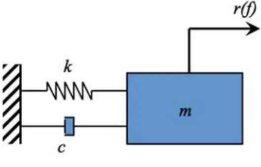
To fix ideas, we can consider the most simple case of a device which is idealized as a simple linear spring-damper-mass system fixed at one end and subjected to an imposed harmonic displacement at the other end (sketched in Figure 1). In the frequency domain, the displacement of this single degree of freedom (SDOF) system, , is given by Lin (1967):
(4)
with:
(5)
where is the frequency. In this equation, , and are the stiffness, mass and damping system parameters (respectively), and the displacement is obtained by solving equation (4), leading to:
(6)
In contrast to a general mechanical problem which is continuous in the space dimension, this simple system has only one spatial degree of freedom.
Figure 1: SDOF system.
Latin American Journal of Solids and Structures 13 (2016) 1203-1227 (7)
which has the amplitude:
(8)
Hence, amplitude of the Frequency Response Function depends non-linearly of the stiffness of the component.
More generally, frequency response function of a discrete system obtain by a finite element anal-ysis or frequency response function of a continuous system could also be considered in this study.
3.2 Stochastic Formulation of the Mechanical Problem
The mechanical system becomes stochastic when stiffness parameters or the loads (or both) are no longer deterministic. In the sequel, random variables will be denoted capitalizing the letter that rep-resents the deterministic variable, hence and in this case for the stiffness and the response amplitude.
The formulation adopted in this study is based on peak amplitudes of the system response. Con-sidering the SDOF device has a random stiffness, the amplitude system response is a random process, which leads to study:
(9)
for a unit forcing function.
In this study, the probability law for the random variable is chosen from the Maximum Entropy Principle (Kapur and Kesavan 1992, Rubinstein and Kroese 2008). This principle states that the uniform probability maximizes the entropy in the case of bounded domain of the random variable.
Thus, the probability density function (PDF) given by the constant value over
is adopted for the random variable , where denotes its mean value and its standard deviation. From the problem description proposed in the previous section, the
set of random processes is and the vector of design parameters is .
4 FORMULATION OF THE RELIABILITY-BASED DESIGN OPTIMIZATION PROBLEM
4.1 Objective Functions
From a design point of view, an interesting objective is to design springs with the lowest stiffness in order to generate significant economical gains due to cheaper material. But another economical inter-esting point is to authorize a large dispersion about the nominal design when building multiple springs, that is do not be strict about the manufacture. Thus, the optimization problem of interest is posed such as the one which minimize the mean stiffness and which simultaneously maximize its stand-ard deviation , to reduce manufacture costs. This leads to a two-objective optimization problem
( ).
4.2 Reliability Constraints
From a design point of view, the amplitude of the vibration response has to respect the bound for the peak level given by the specification, at least within a chosen reliability value . This define the limit state as:
(10)
where denotes the bound for the peak amplitude limit given by the specification and . To focus on main ideas in our problem, the peak limit function is considered deterministic. Thus, we can write the non-failure probability as:
(11)
where denotes the cumulative distribution function of the system amplitude response at the fixed frequency , thus:
(12)
being the probability density function (PDF) of the system and is the left endpoint of the support of .
For a general problem, the distribution function of the system response amplitude is linked to the system random variables. Hence, considering a set of random variables and the system response function , we have:
(13)
Latin American Journal of Solids and Structures 13 (2016) 1203-1227 method. In addition, to handle the continuous limit state linked to the random processes set, it is sampled at fixed frequencies, leading to:
(14)
which are collected in the vector of probabilities.
A possible general way to evaluate numerically this probabilities vector is the Monte Carlo nu-merical simulation method:
1. Choose , , and ;
2. Generate an event ;
3. For a sampling set of , , composed from components, compute for each frequency :
a) ; that is, compute the displacement amplitude for the generated at
step 2 by solving the vibration problem at the frequency ;
b) Evaluate the component of the vector related to the considered
frequency from the Monte Carlo simulation method; that is compute the ratio be-tween the number of displacement amplitude that are lower than the peak limit func-tion and the total number of the element of the event;
4.3 Resulting Formulation
Consequently, the reliability based design optimization problem has the following multi-objective form:
( )
( )
( )
( )
T r max min ,subject to: Prob , for 1,...,
3 , 0
~ Uniform
K K
K j j
K K K
U f u f P j e
K
m s
m s s
ìïï
ï é ù
ï =
-ï ë û
ïïï é < ù³ =
í ë û
ïï
ï > ³
ïï ïïïî x x (15)
with the two-parameter vector ( ).
5 UNCERTAINTIES PROPAGATION RESULT FOR THE SDOF SYSTEM HAVING A STIFFNESS
WHICH FOLLOWS A UNIFORM DISTRIBUTION
For an SDOF problem, there is only one single random variable in the set , and an analytical expression can be derived instead of using a Monte Carlo numerical simulation method. By using
, it is found that (Zwillinger and Kokoska, 2000):
(16)
In this expression, for denotes the roots of the algebraic equation , for
fixed (notice that for a bijective function). By considering a uniform distribution for the stiffness random variable such that:
(17)
having the mean , this produces (Pagnacco et al. 2015):
(18)
where:
denotes the upper envelope of the system response which is given by:
(19)
Latin American Journal of Solids and Structures 13 (2016) 1203-1227 (20)
denotes the domain where there is two roots. It is given by:
(21)
and we defined elsewhere for convenience.
Then, it is possible to evaluate the reliability for a fixed frequency by integrating the PDF given by Equation 18 which leads to:
(22)
such that:
(23)
where . Moreover, it is also possible to invert the integral of the PDF with an unknown upper boundary to find the iso-quantile function:
(24)
which leads to:
with:
(26)
and:
(27)
These two results enable to determine equivalently if the constraint is satisfied -or not- for the optimization problem at a fixed frequency, and frequency-by-frequency. From the first result, the
result is compared to . From the second result, is compared to .
Figure 2: FRF amplitude of a SDOF system having a uniform distribution for the stiffness; the thin line is for the nominal system response; the colored region is for the total amplitude dispersion; the lighted color is
for a probability lower than 75%.
To illustrate these results, we chose a SDOF system having a mean of 3500 N and a standard deviation of 700 N. In the Figure 2, the nominal amplitude in function of the frequency is plotted as well as the total dispersion, and the 75% quantile.
6 OPTIMIZATION
re-Latin American Journal of Solids and Structures 13 (2016) 1203-1227 sulting optimization subproblems are solved by using the Pincus representation formula in conjunc-tion with Nelder-Mead algorithm and the penalty method which deals with the constraints produced by NBI. This leads to the RFNM optimization algorithm (for Representation Formula Nelder-Mead), which permits to find global optima for the Pareto front (Zidani et al. 2013). Explanations about ideas of NBI method and RFNM optimization procedure are given in the appendix section.
For the problem of this work, the NBI first step is to find the solution sets and of both single-objective subproblems, corresponding to the individual global minima of each objectives
and :
(28)
and:
(29)
with the two-parameter vector and where is the admissible domain for the
design-point solutions (the ones that satisfy all constraints):
(30)
In order to apply the RFNM procedure, each constrained single-objective optimization subprob-lem formed by the NBI methodology is transformed into non-constrained optimization subprobsubprob-lem by using the penalty methodology (Haftka and Gurdal 1993). Then, by using the Equation (23), problems to solve are:
(31)
and:
(32)
for:
since boundary on the parameters are handled explicitly with the RFNM procedure. In both these expressions, the constant is the penalty constant that has to be chosen for our application. This
enables to evaluate and to form the utopia point .
Next, NBI consists in making a sequential set of single objective subproblems,
which depends of a parameter and defined by:
(34)
where and:
is the 2 × 2 pay-off matrix;
is a vector of chosen weights for the -th subproblem and such that ,
; and
is a quasi-normal direction which points towards the point in the objective space . It has to be chosen for each application (see the footnote 1 in the next section devoted to the application).
Then, as for the first NBI step, each constrained single-objective optimization subproblem is transformed into non-constrained optimization subproblem by using the penalty methodology:
(35)
since boundary on the parameters are handled explicitly with the RFNM procedure.
Next, unconstrained optimization problems given by Equations 31-32 and 35 of NBI method are solved by the RFNM procedure (Zidani et al. 2013). In this procedure, the Pincus representation formula is used to obtain only a set of guess starting points for the Nelder-Mead algorithm by generating a small finite sample size of pseudo-random numbers for the evaluation of the means. This strategy enables to find global optima. Note that it does not use sensitivities, which avoids drawbacks of the involved penalty methodology and makes it efficient.
However, to ensure a better numerical conditioning, objective functions are scaled and replaced throughout the optimization procedure, such that:
(36)
Latin American Journal of Solids and Structures 13 (2016) 1203-1227
7 APPLICATION: SDOF WITH A SPECIFIC HULL CONSTRAINT FOR SEVERAL RELIABILITY
LEVELS
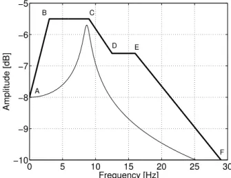
Points A B C D E F
Frequency [Hz] 0 3 9 12.5 16 29
Amplitude [dB] -8 -5.5 -5.5 -6.6 -6.6 -10
Table 1: Coordinates of the points that define the amplitude peak response hull for the optimization problems.
This application is defined from the amplitude peak response hull that corresponds to the line segments delimited by points A to F given in the Table 1. The Figure 3 shows the prescribe amplitude peak response hull, as well as a FRF amplitude corresponding to a deterministic SDOF system which belongs to the permissible region, since it is entirely under the curve delimited by the prescribed hull. For this specified hull, several situations were investigated by choosing different values of the
admis-sible reliability levels: . In addition, we chose to take a unit mass
for the numerical application.
Figure 3: FRF amplitude of one deterministic SDOF system and the available amplitude peak response hull.
In practice, sample size of pseudo-random numbers are chosen for generating from the Pincus representation formula guess points for the Nelder-Mead algorithm (the minimum value seems to be to obtain meaningful results). Moreover, each optimization from the Nelder-Mead algorithm is repeated by using new samples in order to ensure to find at least 3 times the same minima. From our numerical experience with this application, this procedure ensures to catch the global minimum. For a good resolution, a set of 147 points is chosen to construct the NBI boundary
front. For the current application, the scaling factors chosen are , , and
. Another parameter to be chosen is the number of the discretization for the fre-quency range of interest. The Figure 4 shows the results of investigations for three NBI boundary fronts, having , and frequency points of discretization, for a reliability level of 100%. We can observe that there is no difference between the last two discretization, demonstrating that a convergence is achieved. To ensure our application results, we take 1,500 points for this discretization in the following.
Figure 4: NBI boundary front for several discretization of the frequency range of interest.
Since starting guess points for the Nelder-Mead algorithm comes from samples of random varia-bles, the number of evaluations of the mechanical problem varies for each new run. For a relative stopping criteria of in the evolution of the objective function or in the evolution of the param-eters, it is observed that it is approximately an average of 1,000 evaluations for each point of the NBI front.
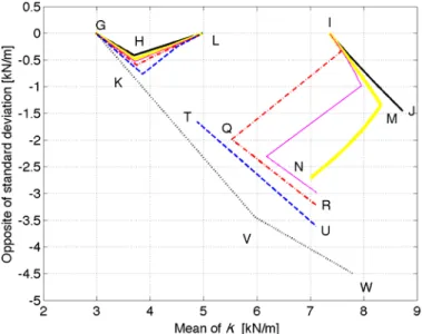
Results of the NBI boundary fronts obtained for each admissible reliability level are collected and reported in the Figure 5. Then, the RFNM optimization procedure leads to the six NBI boundary fronts presented in the Figure 5. For a 100% reliability, the front obtained1 is made of two disjoints parts: the lines segments GH, HL and the line segment IJ. There is no continuity of the front between the point L and the point I since there is no admissible solution for the optimization problem in this
1 Notice that to obtain this NBI front, the normal of the NBI method has to be chosen adequately (we took
for instance), since only the line segments GH and IJ are obtained with the recommendation of Das and
Dennis (1998): . However, it is not a critical difficulty and the standard choice could be also admissible without
Latin American Journal of Solids and Structures 13 (2016) 1203-1227 region. To explain the physical meaning of this solution, we can start from the left point G, corre-sponding to the minimal stiffness that satisfies the optimization constraints. At this design point, the stiffness standard deviation is at its lowest value: it is zero. This is the limit situation where a random system becomes deterministic. So, there is no acceptable uncertainty at this design point. Hence, we consider in this extreme situation that the reliability constraint is respected for any target value. Observing the mechanical system response amplitude helps to better understand the design point G. In fact, the FRF amplitude shown in the Figure 3 is precisely the one of the mechanical system corresponding to this design point G. We can observe in this Figure 3 that the FRF amplitude intersects the available amplitude peak response hull at the null frequency2. It is clear from this figure that giving a non-null standard deviation would leads to a dispersion about the nominal response amplitude, which is impossible since there is no margins between the nominal response amplitude and the amplitude peak response hull at this (null) frequency. In addition, one can see that decreasing this optimal meanLfigure-stiffness value would increase the FRF amplitude over all frequencies, hence at the null frequency too, which is also impossible. This explain the meaning of this solution.
Figure 5: NBI boundary front for several chosen reliabilities: the medium line corresponds to =100%, the thick
line corresponds to =93%, the thin line corresponds to =90%, the dash-dot line corresponds to =87%,
the dashed line corresponds to =83%, the dotted line corresponds to =75%.
On the contrary, increasing the mean stiffness results in a decrease in the amplitude response of the nominal system at all frequencies, therefore at the null frequency too. This allows the nominal system to go away from the forbidden region delimited by the amplitude peak response hull, enabling now some randomness in the response. Thus, increasing the mean stiffness enables the increase of the stiffness standard deviation, as long as the imposed reliability can be satisfied. So, by increasing the
mean, the optimal design solutions travels along the NBI front from the design point G to the design point H (Figure 5) for the 100% reliability level. However, we have to keep in mind that increasing the mean stiffness increases also the resonant frequency of the system. Then, the design point H is a limit situation where it becomes impossible to find an admissible solution by increasing the mean stiffness for a same standard deviation. At this design point H, the admissible system response dis-persion is simultaneously constrained at two distinct frequencies, namely 0 Hz and 12 Hz, as it is shown in the Figure 6-up-left. Next, it becomes necessary to decrease the standard deviation to enable the stiffness increased, up to the point L. At this design point L, the standard deviation becomes null for a maximal stiffness (see Figure 6-up-right). One can note however that these design solutions, between points H and L, do not belongs to the Pareto front since one objective function is deteriorated when traveling through this way.
(a) (b)
(c) (d)
Figure 6: Graphs of the SDOF system FRF amplitude at the design points H (a), L(b), I (c), J (d) for the reliability constraint of 100%; Colored region indicates the total dispersion of the SDOF amplitude,
while the thin line indicates the response of the nominal system.
Latin American Journal of Solids and Structures 13 (2016) 1203-1227 under the constraint hull (see Figure 6-down-left). Then, increasing the stiffness again from this point continued to decrease the amplitude, enabling the possibility of having a non-null, positive, standard deviation. The limit situation becomes now the point J, being the end of the NBI front (see Figure 6-down-right).
Explanations of NBI fronts for the reliability ranging from 93% to 83% are similar. All these fronts share the same left point G and has disjoints parts for the NBI fronts. Differences arise only from the possibility for the SDOF uncertainties to come over the prescribed hull, depending on the required reliability. Frequency response amplitude corresponding to point M and N are presented in Figure 7 for the 93% reliability. One can observe that the point M corresponds to an intersection of the 93% quantile with the constraint hull at 12.5 Hz, while the point N intersects at 4 frequencies, namely 0 Hz, 12.5 Hz, 17 Hz and 29 Hz. Frequency response amplitude corresponding to point Q and R are presented in Figure 8 for the 87% reliability. The point Q corresponds to an intersection of the 87% quantile with the constraint hull at 0 Hz and 12.5 Hz, while the point R intersects at 0 Hz and 29 Hz.
(a) (b)
Figure 7: Graphs of the SDOF system FRF amplitude at the design points M (a) and N (b) for a =93%
reliability. The lighted color region shows the dispersion that respect the reliability constraint (i.e. the region
corresponding to , the darken color extends this region to show the total dispersion of the
SDOF system, while the thin line indicates the response of the nominal system.
(a) (b)
Figure 8: Graphs of the SDOF system FRF amplitude at the design points Q (a) and R (b) for a =87%
reliability. The lighted color region shows the dispersion that respect the reliability constraint (i.e. the region
corresponding to , the darken color extends this region to show the total dispersion of the SDOF system, while the thin line indicates the response of the nominal system.
(a) (b)
Figure 9: Graphs of the SDOF system FRF amplitude at the design points V (a) and W (b) for a =75%
reliability. The lighted color region shows the dispersion that respect the reliability constraint (i.e. the region
Latin American Journal of Solids and Structures 13 (2016) 1203-1227 Figure 10: Pareto front for several chosen reliabilities: the medium line corresponds to =100%, the point
corresponds to =93%, the thin line corresponds to =90%, the dash-dot line corresponds to =87%,
the dashed line corresponds to =83%, the dotted line corresponds to =75%.
Throughout this analysis, it is clear that a filtering is necessary to extract the set of non-domi-nated points from the NBI boundary front, at the exception of the front of the 75% reliability case. The resulting Pareto front is then constituted from simple disjoints parts, as the Figure 10 illustrates it. The 93% reliability being only a line segment and a single point.
8 CONCLUSIONS
A reliability-based design of a mechanical suspension device is discussed in this study. For the sake of simplification and focusing on the main ideas, it is modeled as a SDOF dynamical system and only the stiffness was considered random. For an assumed bound random variable, the MEP gives the stiffness being a uniform distribution. The main constraint to the problem is the prescription of a peak amplitude hull, where the FRF amplitude of the device has to fit, within the band of frequency of interest. Uncertainty propagation is achieved analytically in this situation. Since the design is reliability based, one must also prescribe the desire reliability . The greater is this probability, the most strict is the acceptance of the rules.
interesting problem results and, for some choice of the reliability, a not-connected Pareto curve is obtained, meaning that there is a sub-frequency band where there is no solution for the problem.
References
Avriel, M. (1976), Nonlinear programming: Analysis and methods, Englewood Cliffs, NJ.
Bez, E., Souza de Cursi, E., and M.B., G. (2005), A hybrid method for continuous global optimization involving the representation of the solution. In 6th World Congress on Structural and Multidisciplinary Optimization, Rio de Janeiro. Choi, S., Grandhi, R., and R.A., C. (2007), Reliability-based structural design, Springer.
Das, I. and Dennis, J. (1998), Normal-boundary intersection: a new method for generating pareto optimal point in nonlinear multicriteria optimization problems, SIAM Journal on Optimization, 8:3:631–657.
Haftka, R. and Gurdal, Z. (1993), Elements of structural optimization, Kluwer Academic Publishers, Dordrecht, Netherlands.
Kapur, J. and Kesavan, H. K. (1992), Entropy optimization principles with applications, Academic Press, Inc., London. Lemaire, M. (2009), Structural reliability, Wiley.
Lin, Y. K. (1967), Probabilistic theory of structural dynamics, McGraw-Hill, Inc., New York. Luenberger, D. (1973), Introduction to linear and nonlinear programming.
Nelder, J. and Mead, R. (1965), A simplex method for function minimization, Computer Journal, 7:308–313. Pagnacco, E., Sampaio, R., and Souza de Cursi, E. (2015), Complexity of the response of linear systems with a random coefficient and propagation of uncertainties, Journal of the Brazilian Society of Mechanical Sciences and Engineering, 37:1591–1608. doi: 10.1007/s40430-015-0323-7.
Pincus, M. (1970), A Monte Carlo method for the approximate solution of certain types of constrained optimization problems, Operation Research, 18:1225–1228.
Rubinstein, R. Y. and Kroese, D. P. (2008), Simulation and the Monte Carlo method, John Wiley & Sons, Inc., New Jersey, USA.
Souza de Cursi, E. (2007), Representation of solutions in variational calculus, E. Tarocco; E. A. de Souza Neto; A. A. Novotny , (Org.). Variational Formulations in Mechanics: Theory and Applications. Barcelona , (CIMNE).
Souza de Cursi, E. and Sampaio, R. (2015), Uncertainty quantification and stochastic modeling with matlab, Elsevier, ISTE Press.
Souza de Cursi, E., Bez, E., and Goncalves, M. (2008), A procedure of global optimization and its application to estimate parameters in interaction spatial models. In EngOpt 2008.
Zidani, H., Pagnacco, E., Sampaio, R., Ellaia, R. and Souza de Cursi, E. (2013), Multi-objective optimization by a new hybridized method: applications to random mechanical systems, Engineering Optimization, 45:8: 917–939. doi: 10.1080/0305215X.2012.713355.
Zwillinger, D. and Kokoska, S. (2000), Standard probability and statistics tables and formulae, Chapman & Hall/CRC, New York, USA.
A Procedure to Solve the Multi-Objective Optimization Problem
Latin American Journal of Solids and Structures 13 (2016) 1203-1227 order to be solved by the RFNM procedure. Optimum solutions of this sequence enable to construct a pointwise approximation of the efficient Pareto front.
A.1 NBI method
Multi-objective optimization involves the simultaneous optimization of n incommensurable, and often competing, objectives :
(37)
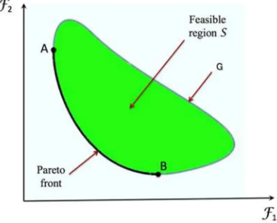
for parameters . In the absence of any preference information, a non-dominated set of solu-tions, termed as Pareto optimal solusolu-tions, is sought. This is illustrated in Figure 11 for the minimi-zation of a two-objective function. The most popular method to solve this problem is the weighted sum approach (Haftka and Gurdal 1993). But this method has the major drawback of not being able to generate an extended set of optimal Pareto solutions even for a uniform distribution of the weighting coefficients. In response to the failure of the weighted sum method, Das and Dennis (1998) have proposed the NBI method, which can produce a collection of even spread points on the Pareto front. NBI works by transforming the multi-objective optimization problem into a set of nonlinear programming subproblems from a geometrically intuitive parameterization. This strategy produces a set of points on the Pareto front, giving an accurate picture of the whole front. This strategy can be considered as the state-of-the-art regarding deterministic methods.
Figure 11: Pareto front for the minimization of two-objective function.
In order to explain the idea of the NBI method, let us define:
the solution vector for the individual function of the optimization problem in the
feasible region, .
the vector of the objective functions evaluated at the solution
the vector of the individual optimal solutions for the objective
functions (i.e., the utopia point or shadow minimum).
the pay-off matrix in which the -th column is :
(38)
In these conditions, the set of the point of , convex combination of , i.e.
, is the so-called Convex Hull Individual Minima (CHIM). This is
illustrated in Figure 12(a) for the minimization problem presented in the Figure 11.
(a) (b)
Figure 12: (a) CHIM representation for a minimization problem of two-objective function; and (b) 7 NBI subproblems to solve.
The purpose of NBI is to find the portion of space that contains the Pareto optimal front. In the Figure 11, this front is reduced to the black curve between the points A (i.e. ) and B (i.e.
) near the axes origin. The algebraic idea behind this approach is simple and evident: the
Latin American Journal of Solids and Structures 13 (2016) 1203-1227 Figure 12(b). Let us denote by the unit normal vector to the CHIM pointing to the origin. Under these conditions , , represents the set of points on this normal. The intersection of the normal and boundary closest to the origin is the global solution of the following problem:
(39)
Note that if the origin is not taken in , the constraint should be written in the form . We obtain a new formulation denoted NBI( ) for the minimization problem:
(40)
The idea is to solve NBI( ) for different values of and find different points of the limit and thus effectively build an approximation of the efficient front. In Figure 12(b), 7 blue arrows, producing 7 points of the Pareto front, illustrates this.
Generally, the vector can be chosen almost normal with negative components (points to the origin), and the results will be the same. For general situations, it is a quasi-normal direction as a linear combination of columns, multiplied by -1 to provide a direction toward the origin:
(41)
where is the all-ones column vector.
(a) (b)
Figure 13: (a) Pareto front for a specific problem of minimization of two-objective function having a non-convex feasible region; and (b) illustration of NBI subproblems generated from a 7 points
But the points thus obtained are not necessarily Pareto optimal points. To illustrate this assertion, the Figure 13 shows the Pareto front and solutions obtained from seven points of CHIM for a specific minimization problem with two-objective function having a non-convex feasible region. In this figure, it is clear that the points numbered 2 to 5 are not Pareto optimal, although they were found by the NBI method. As a consequence, a filtering procedure must be involved in post-processing, once NBI subproblems solutions are produced, in order to obtain the Pareto front.
A.2 Solving NBI subproblems by the RFNM procedure
The set of nonlinear programming subproblem obtained from the NBI method are solved by the RFNM procedure (Zidani et al. 2013). RFNM procedure is a hybrid Nelder-Mead simplex search with integral representation formula of Pincus and genetic algorithm. But it is a procedure to solve an unconstraint optimization problem. Then, constrained sub-problems obtained from the NBI method are first transformed into unconstrained sub-problems by using the penalty method (Luenberger 1973, Avriel 1976, Haftka and Gurdal 1993).
For solving optimization problems, Nelder and Mead (1965) algorithm is well known for its ease of use. It is a simple direct search technique that does not need to take derivatives of the function under exploration. One interesting feature of this algorithm is its ability to handle difficult objective functions such as the one obtained here by using the penalty method. However, it is a local approach. As a consequence, it is very sensitive to the choice of initial points and does not ensure to attain the global optimum. Hence, it is interesting to hybridize it with the formula method of Pincus (1970) and genetic algorithm to generate the initial point.
In the literature, representation formulae have been introduced in order to characterize explicitly solutions to the generic problem:
(42)
where it is assumed that many minima may exist on from which there is a single optimal point . For instance, Pincus (1970) has proposed the representation formula:
(43)
More recently, this representation has been reformulated by Souza de Cursi (2007) as follows: let be a random variable taking its values on and be a function. If these elements are conveniently chosen, then:
(44)
Latin American Journal of Solids and Structures 13 (2016) 1203-1227 for points having values higher than when . The formulation of Pincus corresponds to and this is a convenient choice. The general properties of and are detailed in Bez et al. (2005) and Souza de Cursi et al. (2008) but uniformly distributed is a convenient choice.
In practice, the numerical implementation uses a large value of λ. A finite sample of is gener-ated, according to the chosen probability distribution. This consists in generating admissible points
. In addition, empirical means are used:
(45)