Abstract
D-regions are defined by its non-linear strain distribution over a cross section. Deep beams are an example of D-regions, as most of its load is usually directly delivered to supports by arch mecha-nism. The present paper focus on the Stringer-Panel Method (SPM), an alternative procedure to some well-known methods for designing this type of structure, i.e., strut-and-tie method and finite element method. A manual approach of SPM is presented, by means of a simple principle of dividing a structure on two distinct elements: stringers, which absorb normal forces, and pan-els, which absorb shear forces by membrane action. Two practical examples of deep beams designed using SPM are presented and their overall behavior were investigated by means of non-linear analysis. Obtained results have shown that SPM is a very attrac-tive alternaattrac-tive for analyzing reinforced concrete deep beams.
Keywords
Stringer-Panel Method; D-regions; deep beams; non-linear analy-sis.
Analysis and Design of Reinforced Concrete Deep Beams
by a Manual Approach of Stringer-Panel Method
1 INTRODUCTION
The design of reinforced concrete beams usually considers the Bernoulli’s Hypothesis, which admits a linear strain distribution over the cross section and despises the strains due to shear, because they are very small. Thus, the design for bending can be done by considering the equilibrium in the cross section and the materials’ simplified constitutive relations. The design for shear, on the other hand, can be simply done by a truss analogy. The regions that adopt this hypothesis are commonly de-nominated as B-regions and as this simplification satisfies both equilibrium and compatibility condi-tions these models can be applied for a wide variety of loads and cross section’s geometries (Mitchell and Cook, 1991).
André Felipe Aparecido de Mello a Rafael Alves de Souza b
a Civil Engineer,
Postgraduate Program, State University of Maringa
b Full Professor of Civil Engineering
Department, State University of Maringa
Corresponding author:
http://dx.doi.org/10.1590/1679-78252623
Whatever the plane sections hypothesis and the truss analogy are considerations that simplify the design, they cannot be considered for any part of a structure. Local regions, such as joints, corbels and areas adjacent to application of concentrated forces, produce disturbed and irregular stress and strain distribution, so that compatibility conditions cannot be applied (Hsu and Mo, 2010). In those regions, denominated as D-regions, strains due to shear are significant and their design must consider the disturbed stress field, as it’s not correct to consider that cross sections remain plane and shear stresses are uniform (Mitchell and Cook, 1991).
D-regions have its behavior described by Saint Venant’s Principle, which states that the dis-turbances caused by concentrated forces (static discontinuity) or changes at the cross section’s ge-ometry (geometrical discontinuity) tend to normalize at a distance approximately equal to the cross section’s largest dimension. Figure 1 shows examples of structures classified as D-regions, as the type of discontinuity: geometrical (a) or static (b and c); and the extensions of those regions.
(a) Changes at the cross section (b) Concentrated forces or reactions (c) Deep Beams
Figure 1: Examples of D-regions (NBR 6118, 2014).
Among D-regions, the deep beams can be featured. As shown in Figure 1, due to its dimensions, deep beams are usually an entire D-region. According to American Concrete Institute (ACI), by its standard ACI 318-14 (2014), deep beams are members in which span is lower than 4 times their height (l ≤ 4h), or concentrated loads exist within a distance “2h” from the support’s face. In these structures, besides bending, shear strains are considerable, as most of the load must be directly de-livered to supports (Rogowsky and MacGregor, 1983).
The design of deep beams must consider the non-linear distribution of strain over a cross sec-tion. The consulted standards, from ACI (ACI 318-14, 2014), Brazilian Association of Technical Standards (ABNT) (NBR 6118, 2014), International Federation for Structural Concrete (FIB) (Bul-letin 55, 2010) and European Committee for Standardization (CEN) (EN 1992-1-1, 2004), suggest using Strut and Tie Method (STM) for designing this type of structure and, for non-linear analyses, Finite Element Method (FEM) is recommended.
called Stringer Method and was recommended by CEB-FIP Model Code (1993), in the absence of a more accurate analysis, for designing thin-walled members.
The most important improvements on SPM’s development were reached in the 1990s. From re-searches conducted at Polytechnic University of Milan (Simone, 1998) and Delft University of Technology (Hoogenboom, 1993; 1998), the method’s matrix formulation was obtained. In that same period, the software SPanCAD, a package software capable of analyzing stringer-panel models by elastic and non-linear formulations, was developed (Blaauwendraad and Hoogenboom, 1997; Hoogenboom, 1998). Unfortunately, the development of SPM stopped there and then only a few applications were available in the scientific literature, as the researches led by Tarquini and Sgambi (2003), Wang and Hoogenboom (2004), Souza (2004, 2012), Hauksdóttir (2007) and Refer (2012).
In this context, it can be observed that the main scientific researches focused on SPM’s compu-tational development, not mentioning the method’s manual application, which can be very practical for the most common situations (Souza, 2012). Furthermore, SPM is not well known around the world, as the consulted standards does not mention the method. Except for Denmark, where the method is used on a larger scale, since Danish National Annex to Eurocode 2 (DK NA) (2013) rec-ommends using SPM for designing structures subjected to in-plane stress conditions. Moreover, in the scientific literature, it’s not possible to find experimental data of structures designed by SPM, which, in fact, lacks for verifying its effectiveness.
Thus, this paper’s main objective is presenting a guide for designing reinforced concrete struc-tures by a SPM’s manual approach, by considering two practical examples of deep beams. These structures will be also designed via STM, in order to compare the resultant reinforcement by the distinct approaches. Besides, the designed structures will be analyzed by SPM’s non-linear formula-tions, using SPanCAD software, and by FEM, using ATENA 2D software (v. 5.1.1 – demo version) (2015), so safety and in-service conditions can be verified and compared from two different solu-tions.
2 STRINGER-PANEL METHOD (SPM)
According to Blaauwendraad (1994), SPM is an intermediate model between FEM and STM, and the resultant reinforcement consists of one or more concentrated bands and a web distributed over the structure or at the most of it, usually applied on two orthogonal directions. The basic difference between FEM and SPM is that, while FEM applies the finest mesh possible, SPM seeks to apply the coarsest mesh for a given geometry (Blaauwendraad and Hoogenboom, 2002).
The method is based on Lower Bound Theorem of Plasticity Theory, so, it’s based on the prin-ciple of stablishing a statically admissible stress field, which does not lead the constituent materials to their plastic strengths (Nielsen and Hoang, 2011). Thus, according to Hauksdóttir (2007), SPM can be applied to any material for which that theory is applicable.
disposed on an oblique direction. They must be placed at the structure’s edges or around existing openings, as well as at the lines of support reactions or concentrated loads.
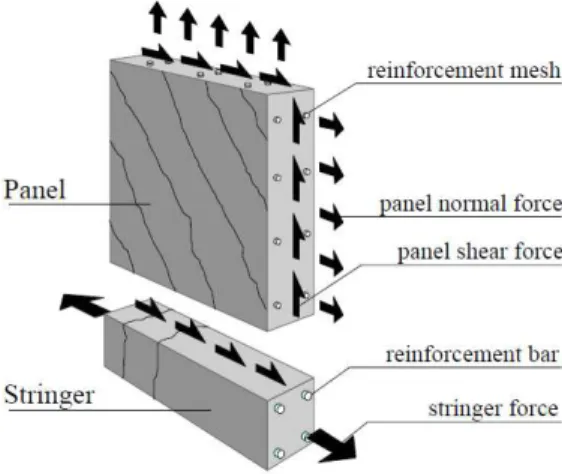
The panels are quadrilateral elements, placed always between four stringers, in order to absorb shear forces. In the most common cases, panels have rectangular geometry, although, for cases where the structure has variable height, they can have trapezoidal shape. Their behavior is based on a membrane element subjected to pure shear, with uniform intensity (Simone, 1998), and the panels’ shear forces must be equilibrated with the axial forces at the adjacent stringers, as shown in Figure 2. Thus, the shear force also acts in the interface between a panel and its adjacent stringers and, according to equilibrium conditions, the stringer’s axial force can increase or decrease linearly (Blaauwendraad and Hoogenboom, 1997).
Figure 2 shows the discretization of a simply supported beam by SPM, as well as the equilibri-um conditions between the stringers and panels. Figure 3 shows a closer look at these elements’ typical configuration and their resultant reinforcements.
Figure 2: Stringer-Panel Model for a beam showing the equilibrium conditions (Blaauwendraad and Hoogenboom, 1997).
Figure 3: Stringers and panels configuration (Blaauwendraad and Hoogenboom, 1997).
makes the model closer to the structure’s real behavior. This type of analysis can be conducted by SPanCAD software, which will be presented in Section 3.
2.1 Determination of Forces in Stringer-Panel Models by Hand Calculations
SPM’s manual approach, despite its simplicity, is not widely spread in the literature. The main researches that apply SPM by hand calculations are those published by Nielsen (1979), Simone (1998), Hauksdóttir (2007), Nielsen and Hoang (2011), Souza (2011, 2012) and Refer (2012). So, in this section, a manual process of obtaining forces in stringer-panel models is presented, as it may result in fast solutions for the most common situations (Souza, 2012).
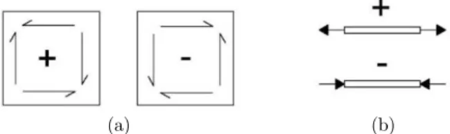
Before starting the process of analysis by SPM, it’s important to adopt a signal convention for the elements’ forces. In this paper, the convention shown in Figure 4 will be adopted. This signal convention is the same considered by Hoogenboom (1998), Simone (1998), Hauksdóttir (2007) and Nielsen and Hoang (2011).
(a) (b)
Figure 4: Signal convention for SPM elements: (a) panels and (b) stringers.
For the most common cases, obtaining the forces is simple. For that, the simply supported deep beam shown in Figure 5 will be used as example. Its length is represented by “l”, its height by “h” and its cross section’s thickness by “t”. This beam is subjected to an external force “P” placed at a distance “x” from the left support. Its effective height (he) is defined by the distance over which the
shear force acts, given as the distance between the upper and lower stringers’ axes.
(a) (b)
In Figure 5a, it can be observed that the deep beam was divided into two panels, surrounded by a total of seven stringers. The forces “RD” and “RF” are the vertical reactions of the left and right
supports, due to the load “P”, and they can be obtained by application of static equilibrium. Con-sidering a section “S1” (Figure 5b) located immediately before the application point of “P” and
con-sidering the equilibrium conditions to the left of this section, the forces in the model can be easily found. In Figure 5b, “FB” is the normal force that compresses the upper stringer at the point “B”,
“FE” is the normal force that tensions the lower stringer at the point “E”, and “v1” and “v2” are the
shear forces that act per unit length on the panels 1 and 2, respectively.
From equilibrium conditions at left of section “S1”, considering the positions of the points “A”
and “B” and that the shear force “v1” acts on the distance between the stringers’ axes (he), the
fol-lowing equations can be written:
0 ; 0 ; 0
1
R R x
D D
Fx F F Fy v M F
B E h B E h
e e
⋅
= = = = = =
å å å (1)
Equation (1) uses the total distance between the stringers’ axes due to the panels’ shear forces also act in the interface of each panel and its adjacent stringers (Blaauwendraad and Hoogenboom, 1997). Besides, it can be observed that the forces “FB” and “FE” are equal in module, although they
have contrary directions, according to those adopted in Figure 5b.
It can also be observed that the product of the vertical reaction by the distance from the chosen point (RD·x) equals to the bending moment (M) acting on section “S1”. Thus, the reaction “RD”
equals to the total shear force (V1) acting on “S1”. Figure 6 shows the model’s internal forces
dia-grams.
(a) (b)
Figure 6: The deep beam model’s internal forces diagrams: (a) shear force and(b) bending moment.
Therefore, comparing the internal forces with the values found on the previous equations, con-sidering simple structures like that shown in Figure 5, it can be deduced that:
M V
-F F ; v
su sl h p h
e e
= = = (2)
being: Fsu: force acting on the upper stringer;
Fsl: force acting on the lower stringer;
Considering the shear force (vp) acting per unit length on a panel, it’s possible to obtain the
shear stress ( p) acting on this panel, according to the following relation:
v p
p t
t = (3)
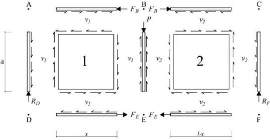
The vertical stringers’ axial forces can be obtained by considering the equilibrium between ex-ternal forces applied to them and the shear forces acting over its lengths. Another way for quantify-ing the forces in a Strquantify-inger-Panel Model is considerquantify-ing a free body diagram, as shown in Figure 7, in which the equilibrium conditions can be easily obtained.
Figure 7: Free body diagram showing the forces acting on the elements of the model.
For statically undetermined problems, in other words, models in which there are more than one panel or more than two stringers in a section, Nielsen and Hoang (2011) suggest to arbitrate the shear force for certain panels, and the choice of these panels is up to the engineer. Then, the shear forces on the other panels can be obtained by vertical or horizontal projections, in order to get a correct total shear force in the section. After that, the stringers’ forces are easily determined by equilibrium conditions. This solution is possible because of ensuring that a plastic redistribution of forces between the model’s elements occurs.
2.2 Design and Verification of Stringers
For designing the stringers, the design values of forces (Nd) for Ultimate Limit State (ULS) must be
considered. In this paper, these forces will be obtained according to ABNT’s standards: NBR 6118 (2014) and NBR 8681 (2003), as shown in the following equation:
d f n k
N = g ⋅g ⋅N (4)
n: additional partial safety factor for D-regions (1,1 ≤ n≤ 1,2);
Nk: characteristic value of the considered force.
The tensioned stringers’ reinforcement is calculated according to Simone (1998), considering that tension forces are resisted exclusively by the steel bars. So, the steel area (As) is obtained by relating the effective force on the stringer and the steel’s yield stress:
, d t s yd N A f = (5)
where: Nd,t: design value of the tension force;
fyd: design value of the steel’s yield stress: “fyd = fyk/ s”;
fyk: characteristic value of the steel’s yield stress.
s: partial safety factor of the steel’s strength: “ s = 1,15” (NBR 6118, 2014).
According to Nielsen and Hoang (2011), the reinforcement should be extended to the entire stringer system, without being reduced or cut. For compressed stringers, it must be checked if its compressive stress ( b) exceeds the stringer’s compressive strength (fs,ef), which can be obtained by
reducing the concrete’s design strength (fcd) by an effectiveness factor (v) and a factor “ c”, which
considers the strength reduction effect by constant loading (Rüsch, 1960). Simone (1998) suggests using an effectiveness factor equal to 1,0 for stringers, so, the stress on a compressed stringer ( b)
should not exceed it’s compressive strength (fs,ef), expressed by the following equation:
s,ef
d,c
b s c cd
c,s
N
f v f
A
s = £ = ⋅a ⋅ (6)
being: Nd,c: design value of the stringer’s compressive force (in module);
Ac,s: the stringer’s cross section area: “Ac,b = hb · t”;
hs: the stringer’s cross section height;
vs: effectiveness factor for the stringers’ compressive strength, which can be considered 1,0;
c: reduction factor for concrete’s peak strength, considering that it’s subjected to constant
loading (Rüsch, 1960). For strengths up to 50 MPa, it can be adopted “ c = 0,85”;
fcd: design value of concrete’s compressive strength: “fcd = fck/ c”;
fck: characteristic value of concrete’s compressive strength;
c: partial safety factor for concrete’s strength: “ c = 1,4” (NBR 6118, 2014).
In cases that the compressive stress in a stringer exceeds the value defined by Equation (6), Simone (1998) suggests a compressive reinforcement, in order to confine the concrete of that region, giving it a superior strength. This reinforcement is disposed on longitudinal(Asc,l) and transverse
directions (Asc,t), in the form of stirrups, and they can be obtained by the following expressions:
(
, ,)
, ,t
/ '
1
;
;
1
4
2
'
/ '
d c c c b ck c conf c c c ck
sc l sc
conf c yd
yd c ck c
conf
N
A
f
s
A
f
A
A
A
f
f
f
a
g
r
f
a
g
a
g
r
æ ö÷ ç ÷ ç ÷ ç ÷ ç ÷ çè ø
-
⋅
⋅
⋅
⋅
⋅
=
=
= ⋅
- ⋅
⋅
where: ’c: modified partial safety factor for concrete’s strength: “ ’c = 1,25· c” for isolated
string-ers, like a simple column, and “ ’c = c” for stringers adjacent to panels;
ρconf: the transverse confinement reinforcement’s geometrical ratio;
øc: diameter of the transverse confinement reinforcement’s steel bars;
s: the transverse confinement reinforcement’s spacing;
Aconf: the concrete’s cross section area confined by the transverse confinement reinforcement;
2.3 Design and Verification of Panels
The panels’ design is based on Equilibrium Plasticity Truss Model (EPTM) (Nielsen, 1967; Lampert and Thürlimann, 1968). The panels behave as a membrane subjected to pure shear, so, by Solid Mechanics, the angle of the principal stresses’ directions ( ) is given by 45o (Hibbeler, 2010), as shown in Figure 8.
Figure 8: Reinforced concrete panel subjected to pure shear.
As the normal stresses on the considered plane are zero ( x = y = 0), the equations of EPTM
can be simplified by:
1
; ;
, ,
c p
p p
sx f sy f
yd x yd y
t l t
r r s t l
l l
⋅
= = = - ⋅ +
⋅
æ ö÷
ç ÷
ç ÷÷
çè ø (8)
where: ρsx; ρsy: the geometrical reinforcement ratio on the directions “x” and “y”, respectively;
fyd,x; fyd,y: design value of steel’s yield stress on the directions “x” and “y”, respectively;
c: principal compressive stress on concrete;
λ: ratio parameter between reinforcement’s strengths on each direction: “λ = fyd,x/fyd,y”.
For the most common cases, in which the steel’s strengths on both directions are the same (fydx
= fydy = fyd), the reinforcement ratio will also be equal. So, Equation (8) can be rewritten by:
; c 2 p
p
sx sy f
yd t
“he” and “le” are considered. Although, if a panel is equilibrated with a tensioned stringer, the panel’s
reinforcement should be distributed over its equivalent dimension, so that the interference between the panel’s and the stringer’s steel bars is avoided. If a panel is in equilibrium with a compressed stringer, and a confinement reinforcement is not present, the steel bars can be distributed over its effective dimensions, attempting that their integral areas must be placed into these distances.
In order to prevent a premature concrete crushing, the stress “ c” must be limited to a value
which considers the softening effect, characterized by crack openings on directions orthogonal to principal tensile stresses. So, the concrete diagonal compressive stress ( c) must be limited to its
effective compressive strength (f’cd), as shown in Equation (10):
c fcd
s £ ¢ (10)
The concrete’s effective strength (f’cd) can be obtained considering STM’s strength parameters
for struts crossed by transverse ties. Table 1 presents the strength parameters for panels, consider-ing the given standard’s parameters for Strut and Tie Models.
Standard Strength parameter (f’cd)
NBR 6118 (2014)
and EN 1992-1-1 (2004) “ cd2 0.60 1 250 fck f = ⋅æççç - ö÷÷÷⋅fcd
÷
çè ø ”
ACI 318-14 (2014) “fce =0.85⋅bs ⋅fc¢”, with “ s = 0.4” and “f’c = fck”
Bulletin 55 (2010) “
1, 5 cd
fck
f¢ =kc ⋅ ”, with “
1/3 30
0.55 0.55
fck
kc = ⋅æççççè ö÷÷÷÷ £
ø ”
Table 1: Concrete’s strength parameters for panels.
For the equations presented in this section, the design values for concrete’s (fcd) and steel’s
strengths (fyd), as well as the design values for loads (Nd) can be obtained according to current
de-sign standards.
3 PRESENTATION OF NON-LINEAR SOFTWARE
In this research, two computer programs were used for non-linear analysis: SPanCAD, which im-plements SPM’s matrix formulation, and ATENA 2D, which is based on FEM.
SPanCAD (Stringer Panel Computer Aided Design) is a software developed by researchers from Delft University of Technology (Blaauwendraad and Hoogenboom, 1997; Hoogenboom, 1998). Actu-ally, SPanCAD is a plugin for the software AutoCAD (Release 14) (1997) and can be downloaded on the authors’ website (Blaauwendraad and Hoogenboom, 1999).
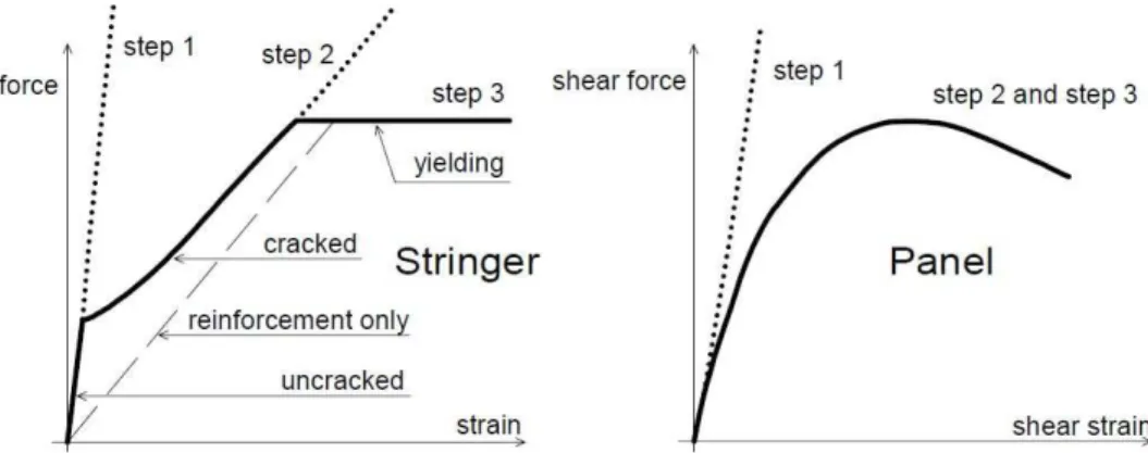
SPanCAD is a simple tool in which non-linear analysis can be made by defining only five pa-rameters. For concrete, it’s enough to inform its Young’s modulus and its compressive and tensile strengths, and for steel, its Young’s modulus and tensile strength. According to Blaauwendraad and Hoogenboom (2002), SPanCAD runs three types of analysis, divided by three steps: in step 1, a linear-elastic analysis is made and the model’s reinforcement can be obtained by this step’s results; in step 2, a non-linear analysis is made, which makes possible a improvement on the stringers’ rein-forcement and a verification of displacements and crack openings for service load combinations; finally in step 3, a model simulation is done, in order to predict its behavior until the collapse load. The elements’ behavior is distinct for each step, as shown in Figure 9.
Figure 9: Non-linear constitutive behavior of stringers and panels in SPanCAD (Blaauwendraad and Hoogenboom, 2002).
ATENA software is developed Cervenka Consulting, a company founded in Czech Republic, and the program is currently on version 5.1.1 (2015). ATENA’s formulations are based on FEM and a good description of this method can be found in Rao (2011). The software presents two ver-sions: ATENA 2D, which can analyze two-dimensional structures, adequate to elements subjected to in-plane stress conditions, and ATENA 3D, which analyses three-dimensional structures. In this paper, ATENA 2D’s demo version was used, which has a limit of 100 finite elements and can be found in the company’s website (Cervenka Consulting, 2015).
For descripting the concrete’s non-linear behavior, ATENA 2D uses SBETA model, which im-plements formulations for behaviors as: tension and compression softening, concrete’s in tension fracture based on non-linear fracture mechanics, biaxial strength failure criterion, compressive strength reduction after cracking and tension stiffening (Červenka et al., 2014). SBETA is made by 20 parameters, which can be automatically defined by informing concrete’s cubic strength (fcu). For
steel’s behavior, it’s possible to consider three models: elastic, bilinear (elastic-perfectly-plastic) and multilinear. The constitutive models used by ATENA 2D are shown in Figure 10.
In non-linear analysis, it’s most appropriate considering the materials’ characteristic strengths. Thus, the safety verification can be done by comparing the ultimate load factor ( u), corresponding
to the structure’s last equilibrium configuration, with the calculated load factor ( calc), which
proper-ties ( m) (Póvoas, 1991). For meeting safety conditions on a structure, these two factors must obey
the following expression:
u calc f n m
g ³ g = g ⋅g ⋅g (11)
with: m = c, for a brittle failure (concrete crushes before reinforcement yielding);
m = s, for a ductile failure (reinforcement yields before concrete crushing);
(a) (b)
Figure 10: ATENA 2D’s constitutive models: (a) concrete (SBETA) and (b) steel (bilinear) (Červenka et al., 2014).
4 PRACTICAL APPLICATION
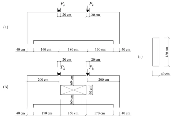
In this research, two practical examples of reinforced concrete deep beams were considered. These structures aim to transfer the concentrated loads of two columns that cannot be extended to the building’s foundation. The first one, named by DB1 (Figure 11a), has a 5-meter span, measured between the support columns’ faces, 180 cm in height and 40 cm in thickness. The second one, named by DB2 (Figure 11b), has basically the same dimensions. The only difference between these two structures is that there are a 160x60 cm opening in DB2’s span, as shown in Figure 11.
The material’s strengths for these structures are defined by 30 MPa for concrete’s compressive strength and 500 MPa for steel’s strength. The design values for concrete (fcd) and steel (fyd)
strengths were calculated according to the ABNT NBR 6118 (2014): “fcd = 21.43 MPa” and “fyd =
434.78 MPa”. The concrete tensile strength is defined by “fctk,inf = 2 MPa” and its initial Young’s
Modulus by “Eci = 30672.46 MPa”. For steel bars, a Young’s Modulus of “Es = 210 GPa” is
(a)
(c)
(b)
Figure 11: Side view of (a) DB1 and (b) DB2 and (c) the cross section’s geometry.
Both concentrated loads (Pk), defined by the forces’ characteristic values that must be
redi-rected to the lower floor’s columns, are divided by a permanent (gk = 300 kN) and a variable (qk =
150 kN) portions. The load combinations for the models were obtained according to ABNT NBR 6118 (2014), by a normal combination (Pu) for Ultimate Limit State (ULS) and by a
quasi-permanent (Ps1) and a frequent (Ps2) combinations for Serviceability Limit State (SLS). The service
load combinations “Ps1” and “Ps2” will be used for checking displacements and crack openings,
re-spectively. They are obtained by the following equations:
(
)
s 1
s 2
1, 4 1,1 693
0, 3 345
0, 4 360
u k k
k k
k k
P g q kN
P g q kN
P g q kN
= ⋅ ⋅ + =
= + ⋅ =
= + ⋅ =
(12)
4.1 Stringer-Panel Models
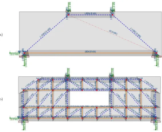
(a)
(b)
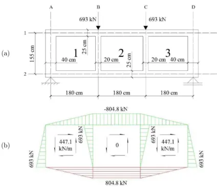
Figure 12: DB1’s analysis by SPM: (a) stringer-panel model and (b) the model’s forces.
The reinforcement calculation adopted the equations showed in sections 2.2 and 2.3, considering the minimal reinforcement ratios suggested by ABNT NBR 6118 (2014). As the stringer’s steel bars must be extended to the beam’s edges, its maximum tension force was taken into account. By prac-tical reasons, the horizontal reinforcement of panels 1 and 3 was extended to panel 2 and a minimal ratio was considered for its vertical reinforcement (ρsy = 0.23). Table 2 presents the elements’
rein-forcement calculation, as well as concrete compression verification, according to the Brazilian standard.
Stringer Area (cm2)
Nd,max
(KN)
As
(cm2)
Adopted reinforcement
c
(MPa)
vb· c·fcd
(MPa)
Compression Check
1 1000 -804.8 - - -8.05 18.21 OK
2 1000 804.8 18.51 6 ø 20 mm - - -
A = D 1600 -693 - - -4.33 18.21 OK
B = C 800 -693 - - -8.66 18.21 OK
Panel p (MPa)
ρsx = ρsy
(%)
As,x
(cm2) As,y
(cm2)
Adopted Reinforcement
(x/y)
c
(MPa) f'cd
(MPa)
Compression Check
1 = 3 1.12 0.26 15.94 18.51 16 ø 12.5 mm /
18 ø 12.5 mm -2.24 11.31 OK
2 0 0 0 0 16 ø 12.5 mm /
18 ø 12.5 mm 0 11.31 OK
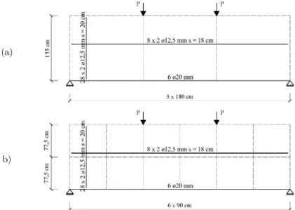
The reinforcement was placed in order to adequate to practical reasons and its configuration is shown in Figure 13. The panel’s reinforcement has a web distribution and its spacing (s) is also shown in Figure 13. From this configuration, two models were defined for non-linear analysis in SPanCAD: model A (Figure 13a), which is the same model adopted for the design, and model B (Figure 13b), which has a better discretization.
(a)
b)
Figure 13: Stringer-panel model and reinforcement for DB1: (a) model A and (b) model B.
For DB2, a model of 24 panels and 64 stringers was considered, as illustrated in Figure 14. For the stringers not present in DB1 model (the central ones), a 10 cm height was adopted. The analy-sis of forces was done for each section, by considering equilibrium on the horizontal direction and the lever arm that each stringer had to absorb the bending moment, as, according to Nielsen and Hoang (2011), it’s possible to arbitrate the stresses in some panels and calculate the remaining ones by projections. The forces in the model are presented in Figure 15, which shows the stringer’s forces on the left side and the panel’s shear forces on the right side, because of the beam’s symmetry.
Figure 15: Forces in DB2’s stringer-panel model.
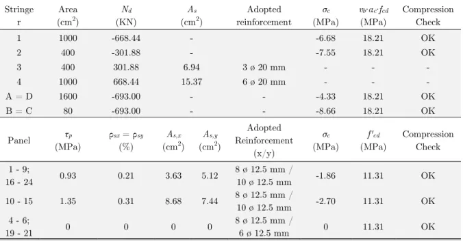
The model was designed in the same way as DB1. The resultant reinforcement is shown in Table 3, in which it’s possible to observe that a continuous reinforcement was adopted to panels, in other words, the most loaded panels’ steel bars were extended to the structure’s edges. Figure 16 illustrates the reinforcement obtained for the DB2, as the model that will be analyzed by SPanCAD.
Stringe r
Area (cm2)
Nd
(KN)
As
(cm2)
Adopted reinforcement
c
(MPa)
vb· c·fcd
(MPa)
Compression Check
1 1000 -668.44 - -6.68 18.21 OK
2 400 -301.88 - -7.55 18.21 OK
3 400 301.88 6.94 3 ø 20 mm - - -
4 1000 668.44 15.37 6 ø 20 mm - - -
A = D 1600 -693.00 - - -4.33 18.21 OK
B = C 80 -693.00 - - -8.66 18.21 OK
Panel p
(MPa)
ρsx = ρsy
(%)
As,x
(cm2) As,y
(cm2)
Adopted Reinforcement (x/y) c (MPa) f'cd (MPa) Compression Check
1 - 9;
16 - 24 0.93 0.21 3.63 5.12
8 ø 12.5 mm /
10 ø 12.5 mm -1.86 11.31 OK
10 - 15 1.35 0.31 8.68 7.44 8 ø 12.5 mm /
10 ø 12.5 mm -2.70 11.31 OK 4 - 6;
19 - 21 0 0 0 0
8 ø 12.5 mm /
6 ø 12.5 mm 0 11.31 OK
Table 3: Design and verification of DB2 model.
4.2 Strut-and-Tie Models
For comparing the resultant reinforcement, the deep beams can be analyzed via STM. A general formulation of this method can be found in Schlaich et al. (1987) and Wight and MacGregor (2012). By practical reasons, CAST software (Tjhin and Kuchma, 2004) was used for obtaining these struc-ture’s strut-and-tie models. In order to obtain a more consistent comparison, the chosen models are very similar to those obtained in SPM’s analysis, as shown in Figure 17.
(a)
(b)
Figure 17: Strut and tie models for the studied deep beams: (a) DB1 and (b) DB2.
For DB1’s model (Figure 17a), it can be observed that the forces in the upper strut and the lower tie are equal to those obtained by SPM (Figure 12b). This is certainly due to the fact that, in both models, these elements are calculated considering only the bending moment. Thus, for DB1, both models resulted in the same reinforcement for the lower tie. The only difference between these models is that, while for SPM it’s possible to obtain the distributed reinforcement, for STM, just a minimal web reinforcement would be required. For both DB1 and DB2, the minimal reinforcement ratios were defined by “ρsx = 0.2” and “ρsy = 0.23”.
ties. For example, for the vertical ties loaded by 260 kN, two 20 mm diameter steel bars would be required. Besides, according to design standards, a minimal web reinforcement would also be neces-sary.
Table 5 presents a comparison, in terms of total weight, between the resultant reinforcement of DB1’s and DB2’s distinct approaches, whereas folds and losses were not taken into account. It can be noted that in both structures, SPM and STM resulted in the same reinforcement for the main ties or stringers. Otherwise, STM resulted on less distributed reinforcement than SPM, due to a minimal ratio consideration. Unlike DB2’s SPM model, STM’s would result in a less practical rein-forcement, due to its vertical ties reinforced by 20 mm diameter steel bars.
Deep beam Model Stringer/Tie Web reinforcement (x) Web reinforcement (y) Weight (kg)
DB1 SPM 6 ø20 mm (540 cm) 16 ø12.5 mm (540 cm) 56 ø12.5 mm (180 cm) 260,2 STM 6 ø20 mm (540 cm) 24 ø10 mm (540 cm) 68 ø10 mm (180 cm) 235,4
DB2
SPM 9 ø20 mm (540 cm) 16 ø12.5 mm (540 cm) 16 ø12.5 mm (180 cm)
64 ø12.5 mm (180 cm)
32 ø12.5 mm (55 cm) 397,5
STM
9 ø20 mm (540 cm)
16 ø10 mm (540 cm) 20 ø10 mm (180 cm)
48 ø10 mm (180 cm)
24 ø10 mm (55 cm) 305 8 ø20 mm (180 cm)
2 ø12.5 mm (540 cm)
2 ø10 mm (180 cm)
Table 4: The deep beams’ design models comparison.
5 NON-LINEAR ANALISYS
The designed deep beams were analyzed non-linearly by SPanCAD software, in order to verify the mid-span’s vertical displacement for quasi-permanent load combination (Ps1), the crack openings for
frequent load combination (Ps2), the load that causes the first crack opening and the load that
causes the lower reinforcement’s yielding. For obtaining a comparison of SPanCAD’s results with a more realistic solution, these same designed structures were analyzed by FEM, using ATENA 2D software.
The same reinforcement obtained by SPM’s manual approach for DB1 (Figure 13) and DB2 (Figure 16) was defined on ATENA 2D. SBETA constitutive model was considered for concrete by defining “fcu = fck/0.85 = 35.3 MPa”, according to SBETA’s general formulation (Červenka et al.,
2014). Besides, exponential crack opening law, fixed crack model and Hyperbole A tension-compression interaction were considered. The bilinear model was adopted for steel bars and its strength and Young’s Modulus were defined in the beginning of this section.
The models were defined considering their axis of symmetry, in order to analyze the structure by an adequate number of finite elements. 24 load steps with 15 kN increments were considered, which totals the load of combination “Ps2” (360 kN) and, after that, more load steps with 30 kN
5.1 SPanCAD’s Solutions
DB1’s non-linear analysis conducted by SPanCAD for model A resulted in a 1.2 mm mid-span’s displacement and a 0.016 mm maximum crack opening and, as cracks were placed on the lower stringer, it can be deduced that the they formed by bending. For model B, half of that displacement (0.6 mm) and a 0.1 mm maximum crack opening were obtained and, as these cracks appeared in the panels, it can be concluded the they formed by shear. DB1 models’ in-service behavior is pre-sented in Figure 18.
Model A: displacements Model A: crack opening
Model B: displacements Model B: crack opening
Figure 18: In-service behavior of DB1’s models obtained by SPanCAD.
For obtaining the DB1’s failure load, simulations for both models were done and SPanCAD re-sulted on 945 kN for model A and 1080 kN for model B. These loads represent the lower stringer’s yielding, which can be characterized as a ductile failure. The safety verification for both models satisfies the condition presented in Equation (11). The load-displacement diagrams for simulation of DB1’s models are shown in Figure 19.
(a) (b)
Figure 19: Load-displacement diagrams for DB1 simulation in SPanCAD (a) model A and (b) model B.
Displacements Crack opening
Figure 20: In-service behavior of DB2’s model obtained by SPanCAD.
5.2 ATENA 2D’s Solutions
DB1’s non-linear analysis performed by ATENA 2D resulted in a 1.32 mm displacement for load combination “Ps1” (345 kN). For “Ps2” (360 kN), cracks with a 0.22 mm maximum opening appeared
on the bottom of the beam, bellow the load application points. These results are presented in Figure 22. Figure 23 represents the load step corresponding the 1170 kN loading, in which occurs the lower reinforcement’s yielding. It can be observed that the structure has a ductile failure, as its strains (Figure 23a) exceeded the steel limit (2,38∙10-3) and concrete stresses on top of the beam reached 23 MPa (Figure 23b).
(a) (b)
Figure 22: DB1’s in-service behavior obtained by ATENA 2D: (a) displacements (in meters) for 345 kN loading and (b) crack openings (in meters) for 360 kN loading.
(a) (b)
Figure 23: DB1’s failure by the lower reinforcement yielding: (a) strains on “x” direction and (b) normal stresses (in MPa) on “x” direction.
Figure 24: DB1’s load-displacement diagram for ATENA 2D’s simulation.
DB2’s non-linear analysis made in ATENA 2D resulted in a 1.44 mm mid-span’s displacement for 345 kN loading, and a 0.3 mm maximum crack opening for 360 kN loading, located bellow the structure’s opening, as presented in Figure 25. Figure 26 represents the 1290 kN load step, in which occurs a ductile failure of the structure, as the steel bars are subjected to high strains (Figure 26a) and concrete stresses are up to 23.3 MPa (Figure 26b).
(a) (b)
Figure 25: DB2’s in-service behavior obtained by ATENA 2D: (a) displacements (in meters) for 345 kN loading and (b) crack openings (in meters) for 360 kN loading.
(a) (b)
Figure 27 shows the load-displacement diagram for the DB2 simulation in ATENA 2D, in which the yellow point represents the load step that the first cracks appeared (285 kN) and the red point, the lower reinforcement’s yielding load (1290 kN).
Figure 27: DB2’s load-displacement diagram for ATENA 2D’s simulation.
5.3 Comparison Between SPanCAD’s and ATENA 2D’s Results
Table 5 presents a comparison between SPanCAD’s and ATENA 2D’s results. Information about vertical displacements, cracking and ultimate loads can be compared. There is also a comparison of the peak displacements of the simulations’ diagrams, which can be defined by the maximum mid-span displacements obtained for the ultimate load.
Consideration SPanCAD ATENA 2D Variation (%)
DB1
Mode
l A
Mid-span displacement (in mm) for “Ps1” 1.2 1.32 -9.1
Maximum crack opening (in mm) for “Ps2” 0.016 0.22 -92.7
Concrete cracking load (kN) 554.4 270 +105.3 Lower reinforcement yielding load (kN) 945 1170 -19.2
Peak displacement (mm) 13 8.9 +46.1
DB1
Mode
l B
Mid-span displacement (in mm) for “Ps1” 0.6 1.32 -54.5
Maximum crack opening (in mm) for “Ps2” 0.092 0.22 -58.2
Concrete cracking load (kN) 346.5 270 +28.3 Lower reinforcement yielding load (kN) 1080 1170 -7.7
Peak displacement (mm) 12.5 8.9 +40.4
DB2
Mid-span displacement (in mm) for “Ps1” 0.9 1.44 -37.5
Maximum crack opening (in mm) for “Ps2” 0.2 0.3 -33.3
Concrete cracking load (kN) 242.55 285 -14.9 Lower reinforcement yielding load (kN) 1300 1290 +0.8
Peak displacement (mm) 9 8.6 +4.7
For comparing the results, Table 5 presents a variation parameter, which is given by the follow-ing expression:
(%) 1 100
2
SPanCAD Variation
ATENA D
æ ö÷
ç ÷
=çç - ÷÷⋅
çè ø (13)
It can be observed that the DB1’s model A showed a better approximation for the mid-span displacement than model B and, for the other considerations, model B presented better results than model A, mostly for concrete’s cracking load. The peak displacements obtained for these two models were very close, but relatively distant from that showed by ATENA 2D.
DB2’s analysis showed a better approximation for cracking and ultimate loads, as for the peak displacements. When considering the crack openings for both deep beams, SPanCAD presented results somewhat divergent to ATENA 2D.
6 CONCLUSIONS
This paper’s main objective was to present the analysis and design process of deep beams through a manual approach of SPM. In Section 2.1, it was shown that, for structures that present only static discontinuities, as DB1, the determination of forces can be quickly done through the application of Statics. In cases where geometrical discontinuities exist, which can lead to a statically undetermined model, as DB2, it’s possible to arbitrate shear stresses in some panels and calculate the remaining ones via horizontal or vertical projections (Nielsen and Hoang, 2011).
The practical examples showed that SPM is a method of easy application, as it is a very attrac-tive alternaattrac-tive for analyzing reinforced concrete deep beams and it results in a model as simple as STM. As shown in Section 4, the main difference between these two methods is that, while STM results in a more concentrated reinforcement in the considered ties, SPM can result in a more dis-tributed one, by calculating a web reinforcement for the considered panels.
The conducted non-linear analyses showed that SPanCAD, as a simple software that depends on the definition of only five parameters, presented close results to ATENA 2D, especially for the ultimate loads. Safety and in-service conditions for both deep beams could be verified through the non-linear analyses and the results showed that SPM provided a good solution for designing these structures. However, further investigations need to be done, in order to analyze the behavior of structures designed by SPM by an experimental program, so an adequate comparison between SPanCAD’s solutions and experimental data can be made.
References
ACI 318-14 (ACI) (2014). Building code requirements for structural concrete.
Argyris, J.H., Kelsey, S. (1960). Part I: General Theory, in: Energy Theorems and Structural Analysis. Butterworths (London).
AUTODESK (1997). AutoCAD for Windows. Release 14.
Blaauwendraad, J., Hoogenboom, P.C.J. (1999). SPanCAD’s website. (http://homepage. tudelft.nl/p3r3s/spancad/ index.html) (accessed 1.19.15).
Blaauwendraad, J., Hoogenboom, P.C.J. (2002). Design instrument SPanCAD for shear walls and D-regions, in: FIB Congress, 1., 2002, Osaka.
Cervenka Consulting (2015). Atena 2D for Windows. v. 5.1.1 – demo version.
Cervenka Consulting (2015). ATENA’s website (http://www.cervenka.cz/products/atena/) (accessed 10.23.15).
Červenka, V., Jendele, L., Červenka, J. (2014). ATENA Program Documentation Part 1: Theory.
DS/EN 1992-1-1 DK NA:2013 (DS) (2013). National Annex to Eurocode 2: Design of concrete structures - Part 1: General rules and rules for buildings.
EN 1992-1-1 (CEN) (2004). Eurocode 2: Design of concrete structures - Part 1: General rules and rules for buildings. ENV 1992-1-1 (BSi) (1992). Eurocode 2: Design of concrete structures - Part 1: General rules and rules for buildings. FIB Bulletin 55 (CEB-FIP) (2010). Model Code 2010.
Hauksdóttir, B. (2007). Analysis of a reinforced concrete shear wall, Master’s Thesis, Technical University of Den-mark, Denmark.
Hibbeler, R.C. (2010). Mechanics of Materials, 7th ed. (In Portuguese), Pearson Prentice Hall (São Paulo).
Hoogenboom, P.C.J. (1993). The Stringer-Panel Model, Master’s Thesis (In Dutch), Delft University of Technology, The Netherlands.
Hoogenboom, P.C.J. (1998). Discrete elements and nonlinearity in design of structural concrete walls, Doctoral The-sis, Delft University of Technology, The Netherlands.
Hsu, T.T.C., Mo, Y.L. (2010). Unified theory of concrete structures, 1st ed., John Wiley and Sons (Chichester). Kaern, J.C. (1979). The stringer method applied to discs with holes, in: IABSE Colloquium on Plasticity in Rein-forced Concrete, 29., Copenhagen.
Lampert, P., Thürlimann, B. (1968). Report no. 6506-2: Torsion tests of reinforced concrete beams (In German), Swiss Federal Institute of Technology in Zurich.
Mello, A.F.A. (2015). Analysis and design of reinforce concrete deep beams using Stringer-Panel Method, Master Thesis (in Portuguese), State University of Maringá, Brazil.
Mitchell, D., Cook, W.D. (1991). Design of disturbed regions, in: IABSE Colloquium on Plasticity in Reinforced Concrete, 62., 1991, Sttutgart.
Model Code 1990 (CEB-FIP) (1993). Design Code.
NBR 6118 (ABNT) (2014). Design of concrete structures: procedure (in Portuguese). NBR 8681 (ABNT) (2003). Actions and safety in structures: procedure (in Portuguese).
Nielsen, M.P. (1967). On shear reinforcement in reinforced concrete beams (In Danish), Bygningsstatiske Meddelelser 38: 33–58.
Nielsen, M.P. (1971). On the Strength of Reinforced Concrete Discs, Acta polytechnica Scandinavica: Civil engineer-ing and buildengineer-ing construction series 70, Danish Academy of Technical Sciences (Copenhagen).
Nielsen, M.P. (1979). Some examples of lower-bound design of reinforcement in plane stress problems, in: IABSE Colloquium on Plasticity in Reinforced Concrete, 29., 1979, Copenhagen.
Nielsen, M.P., Hoang, L.C. (2011). Limit analysis and concrete plasticity, 3rd ed. CRC Press (Boca Raton).
Póvoas, R.H.C.F. (1991). Non-linear models of analysis and design of reinfoced concrete laminar structures including deferred effects, Doctoral Thesis, University of Porto, Portugal.
Rao, S.S. (2011). The Finite Element Method in Engineering, 5th ed. Elsevier (Burlington).
Rogowsky, D.M., MacGregor, J. G. (1983). Structural engineering report no. 110: shear strength of deep reinforced concrete continuous beams, University of Alberta.
Rüsch, H. (1960). Researches toward a general flexural theory for structural concrete, Journal of the American Con-crete Institute 32.
Schlaich, J., Schäfer, K., Jennewein, M. (1987). Toward a consistent design of structural concrete, PCI journal 32: 74–150.
Simone, A. (1998). Design of reinfoced concrete structures by the Stringer and Panel Model, Doctoral Thesis (In Italian), Polytechnic University of Milan, Italy.
Souza, R.A. (2004). Structural concrete: analysis and design of discontinuous elements, Doctoral Thesis (In Portu-guese), University of São Paulo, Brazil.
Souza, R.A. (2011). Report of short term postdoctoral internships accomplished at Swiss Federal Institute of Tech-nology in Lausanne (Switzerland) and Delft University of TechTech-nology (The Netherlands) (In Portuguese).
Souza, R.A. (2012). Stringer and Panel Method manual and computational approach for analysis and design of rein-forced concrete walls (In Portuguese), in: Brazilian Concrete Congress, 54., 2012, Maceió.
Tarquini, G., Sgambi, L. (2003). Stringer Panel Method: a discrete model to project structural reinforced concrete elements, in: International Structural Engineering Construction Conference, 2., 2003, Rome.
Tjhin, T.N., Kuchma, D.A. (2004). CAST (Computer Aided Strut and Tie) for Windows. v. 0.9.11.
Vecchio, F.J., Collins, M.P. (1986). The modified compression-field theory for reinforced concrete elements subjected to shear, ACI Structural Journal 83: 219–231.
Wang, Q., Hoogenboom, P.C.J. (2004). Nonlinear analysis of reinforced concrete continuous deep beams using stringer-panel model, Asian Journal of Civil Engineering 5: 25–40.