An ASABE Conference Presentation
Paper Number:
ASABE staff will complete
Modeling runoff with AnnAGNPS model in a small agricultural
catchment, in Mediterranean environment
António Canatário Duarte
College of Agriculture/IPCB, Apartado 119, 6001-909 Castelo Branco, Portugal,
CEER-Biosystems Engineering, Tapada da Ajuda, 1349-017, Lisboa, Portugal
acduarte@ipcb.pt
Luciano Mateos Iñiguez
IAS/CSIC, Apartado 4084, 14080 Córdoba, Spain, ag1mainl@uco.es
Elias Fereres Castiel
Cordoba University, University Campus of Rabanales, 14071 Córdoba, Spain,
ag1fecae@uco.es
21st Century Watershed Technology Conference and Workshop
Bari, Italy
May 27th- June 1st, 2012
Abstract
Agricultural activities, as part of the natural resource management practice, impact soil and water quality at the watershed or catchment level. Field monitoring is often used to evaluate and acquire knowledge of the impacts of management practices on productivity and environment. Computer simulation models, after calibrated and validated, provide an efficient and effective alternative for evaluating the effects of agricultural practices on soil and water quality at the watershed level. The main objective is calibrate and validate the AnnAGNPS model relatively to runoff and peak flow using five hydrologic years data, for the rain and irrigation season. The study watershed is located in Portugal, and covers an area of 189 ha, divided into 18 fields belonging to four farmers. The climate is typically Mediterranean with continental influence, and the main crops are oat, tobacco, sorghum and maize. The calibration was done manually, but in a systematic away, in order to select values for the statistical parameters so that the model closely simulates runoff and peak flow. The results obtained in calibration and validation of the AnnAGNPS model, confirm a good or very good performance to simulate the peak flow and runoff volume at daily or event scale, in rainfall season. Also, the obtained results are a good indication of the validity of AnnAGNPS model to simulate runoff in irrigation to larger periods of time, for example irrigation season.
Keywords
1. Introduction
Agricultural activities as part of the natural resource management practice impact soil and water quality at the watershed or catchment level (Wani et al., 2003; Twomlow et al., 2008). Soil and water conservation practices also help in reducing the loss of chemicals in runoff and in maintaining water quality (Sahrawat et al., 2005; Berry et al., 2003). Non-point source (NPS) pollution is an important environmental and water quality management problem, closely related with hydrologic behavior of the territorial unit (Arnold et al., 1998). In this context, watershed is the basic unit of all research, development and policy-making activities related to water at present. Field monitoring is often used to evaluate and acquire knowledge of the impacts of management practices on productivity and environment. However, field research can be prohibitively costly and time consuming to perform across all possible landscape, climate, management practice, and cropping system combinations (Chung et al., 1999; Davis et al., 2000). Computer simulation models provide an efficient and effective alternative for evaluating the effects of agricultural practices on soil and water quality at the watershed level (He, 2003). Prior to this assessment, these models need to be properly calibrated and validated using hydrologic and water quality data of a basin. It is important to understand not only the level to which model prediction errors are affected by the precision of spatial input data, but also the mechanisms involved in these changes (Chaplot, 2005). Given the multiplicity of hydrological models that simulate non point pollution, our selection for this study was for to the AnnAGNPS model (Cronshey and Theurer, 1998), due to its features well adapts to our objectives. In addition, AnnAGNPS has been used and calibrated in variety of conditions (Baginska et al., 2003; Grunwald and Norton, 2000; Yuan et al., 2001).
For this study, the main objective is calibrate and validate the AnnAGNPS model relatively to runoff and peak flow using five hydrologic years data, for the rain and irrigation season (only runoff), in a small agro-forestry basin under mediterranean climatic conditions.
2. Materials and methods
2.1. The AnnAGNPS model
Several available hydrologic models were evaluated and the AnnAGNPS model (Cronshey and Theurer, 1998) was selected as the simulation tool to be used in this study. AnnAGNPS model is a joint Agricultural Research Service (ARS) and Natural Resources Conservation Service (NRCS) suite of computer models developed to predict nonpoint source pollutant loadings within agricultural watersheds. Within AGNPS, AnnAGNPS is a continuous-simulation, mixed-land use, watershed-scale computer model designed to predict the origin and movement of water, sediment, and chemicals at any location in agricultural watersheds. The model estimates erosion caused by different processes such as sheet and rill, tillage induced gullies, classical gullies, and streambed and bank sources (Bingner et al., 2010). In AnnAGNPS the catchment area is divided into individual slopes (so-called cells), which are directly connected to the river network by potential flow paths. The cells and any potential flow paths are defined automatically based on the digital elevation model (DEM). Each cell has homogeneous vegetation and soil characteristics allocated by the GIS interface based on the prevailing soil type and vegetation (Kliment et al., 2008). AnnAGNPS input accepts five types of land use identifiers (cropland, pasture, forest, rangeland and urban), and only the predominant land use and management are used to represent each AnnAGNPS cell. Output parameters such as runoff, sediment, nutrients and pesticides are selected by the user for the desired watershed source locations (specific cells, reaches, feedlots, gullies and point sources) for simulation duration source accounting.
2.1. Watershed characterization and input parameters
Location of the watershed
The study watershed is located within the Idanha Irrigation Scheme, Idanha-a-Nova, Portugal, near the border with Spain and just north of the Tejo river (Figure 1). The study catchment covers an area of 189 ha; It is divided into 18 fields belonging to four farmers. About one third (31%) of the catchment is not irrigable and is now devoted to a young cork tree forest (10 years) (Duarte, 2006).
Figure 1 - Location of the study watershed.
Soils
The major physical and chemical properties needed by the AnnAGNPS model for each soil layer include layer depth, texture, field capacity, wilting point, organic matter, pH, bulk density, saturated conductivity, structure code, soil hydrologic group and soil erodibility factor. Most of the soil types in the watershed are classified as silty loam. According to the FAO classification system (FAO, 1998), the predominant soil classes are Cambisols and Luvisols, originated from deposits of the tributaries of the Tagus river. Other soil class in the watershed is Fluvisols, originated by alluvial deposits of the main creak that crosses the watershed. An impermeable soil layer underlies the three soil classes at approximately 0.4 m in depth, which greatly determines the hydrology of the watershed. Both the A and B horizons of soils across the catchment have a sandy loam texture.
Topography and watershed schematization
The watershed has 189 ha and 28 natural channels with density 12.2 m ha-1 and fluvial hierarchy of three levels. Altitude varies from 248 m, in a plateau north east, to 212 m at the control section. The slopes are between 0 and 4%, thus the topography is flat to slightly sloppy.
The resolution of the DEM is affects the delineation of watersheds which in turn would influence models’ prediction quality Kalin et al. (2003). Two DEMs with resolutions of 1 and 5 meters were generated by digitizing existing cartographic information at 1:2500 scale. Critical source area (CSA) and minimum source channel length (MSCL) are the input parameters to TOPAZ (Garbrecht and Martz, 1995) which controls the number and size of sub-watersheds and extent of the channel network, respectively. CSA is the minimum upstream drainage area below which a source channel can be initiated and maintained. MSCL is the minimum acceptable length for a source channel (FitzHugh and Mackay, 2000). The selection of the combination of CSA/MSCL values that best represented the observed watershed characteristics were obtained by a trial-and-error process and the values adopted were 3.0 ha and 80.0 meters for CSA and MSCL respectively. Using these values, the study basin was subdivided into 28 sub-watersheds, 67 cells, and 28 reaches (Duarte et al., 2005).
Crops
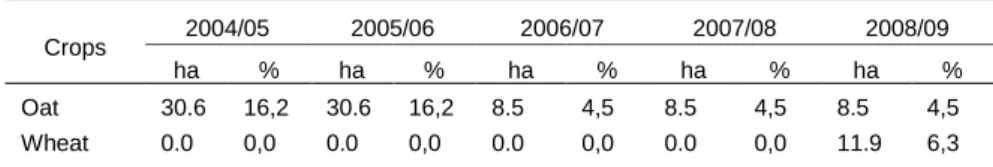
In the Tables 1 and 2 we can see that, both winter and irrigation crops, has been a trend to an increase in the fallow area, most evident in the irrigated crops. This reality is explained in large part by CAP (Common Agricultural Policy) contingencies, and the support system to farmers inherent to this policy.
Table 1 – Area and winter crops in each hydrologic year during the period of analysis.
Crops 2004/05 2005/06 2006/07 2007/08 2008/09 ha % ha % ha % ha % ha % Oat 30.6 16,2 30.6 16,2 8.5 4,5 8.5 4,5 8.5 4,5 Wheat 0.0 0,0 0.0 0,0 0.0 0,0 0.0 0,0 11.9 6,3 N E W S Idanha-a-Nova County Tagus River LEGEND 100 0 100 200 Kilometers SPAIN PORTUGAL # Study watershed
Meadow 0.0 0,0 0.0 0,0 9.8 5,2 0.0 0,0 0.0 0,0 Grass 1.9 1,0 1.9 1,0 6.1 3,2 6.1 3,2 6.1 3,2 Oak/grass 58.6 31,0 58.6 31,0 58.6 31,0 58.6 31,0 58.6 31,0 Fallow 97.9 51,8 97.9 51,8 106.0 56,1 115.9 61,3 103.9 55,0
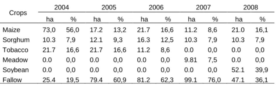
The area values in percentage in the Table 2, are calculated relatively to the agricultural area in the study basin, in other words, excluding the area of oak/grass.
Table 2 – Area and irrigated crops in each year during the period of analysis.
Crops 2004 2005 2006 2007 2008 ha % ha % ha % ha % ha % Maize 73,0 56,0 17.2 13,2 21.7 16,6 11.2 8,6 21.0 16,1 Sorghum 10.3 7,9 12.1 9,3 16.3 12,5 10.3 7,9 10.3 7,9 Tobacco 21.7 16,6 21.7 16,6 11.2 8,6 0.0 0,0 0.0 0,0 Meadow 0.0 0,0 0.0 0,0 0.0 0,0 9.81 7,5 0.0 0,0 Soybean 0.0 0,0 0.0 0,0 0.0 0,0 0.0 0,0 52.1 39,9 Fallow 25.4 19,5 79.4 60,9 81.2 62,3 99.1 76,0 47.1 36,1
Climate
The climate in this region is typically Mediterranean with continental influence. The mean annual of precipitation is 781 mm (data from 1961 to 1986), with a dry and warm period during the summer season. The mean daily temperature varies between 8.3 oC in January and 24.5 oC in August, thermal amplitude proper to the regions with a strong interiority (Duarte, 2006).
For the climatic file, eight parameters were required for each day: date, daily maximum temperature, daily minimum temperature, precipitation, dew point temperature, percent sky cover, wind speed and wind direction. Header data in the file included location latitude for estimation of solar radiation and daily precipitation over a period of 2 years. A value of 31.2 mm was calculated (Gumbel method; Gumbel, 1958) for the daily precipitation for a period 2 years.
The hydrological station
A hydrological station was constructed and installed in 2004 at the outlet of the catchment (39º50’48’’ N, 7º10’00’’ W). The station consisted of a long-throated flume (with a triangular control section for shallow water conditions and a triangular/trapezoidal section for deep water conditions) designed and calibrated following the procedure described by Bos et al. (1991). An ultrasonic sensor (“The Probe”, manufactured by Milltronics, Siemens Milltronics Process Instruments Inc., Ontario, Canada) connected to a datalogger continuously measured and recorded the water level at the flume.
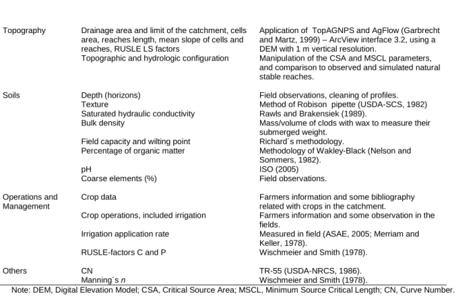
In summary, Table 3 lists the main input parameters commonly used in AnnAGNPS simulations.
Table 3 – AnnAGNPS Input parameters and methods used in their evaluation. Group of
parameters
Imput variables Methods
Climate Daily rainfall
Daily maximum and minimum temperatures, wind direction and speed, daily percentage cloud cover and dew point temperature. Annual distribution EI30
Type of rainfall distribution (TR-55)
Two year 24 hour precipitation
Measurements at the Ladoeiro (INAG, 2008) and Ribeiro de Freixo satations (data not publicated). Measurements at the Ribeiro de Freixo station (data not published).
Calculated with measured data, from Ladoeiro data (INAG, 2008), and the methodology described in Wischmeier and Smith (1978) . Comparison with the 24 h rainfall distribution curve calculated with the data from Ladoeiro station (INAG, 2008)
Gumbel method (Gumbel, 1958) applied to the data from Ladoeiro station (INAG, 2008).
Topography Drainage area and limit of the catchment, cells area, reaches length, mean slope of cells and reaches, RUSLE LS factors
Topographic and hydrologic configuration
Application of TopAGNPS and AgFlow (Garbrecht and Martz, 1999) – ArcView interface 3.2, using a DEM with 1 m vertical resolution.
Manipulation of the CSA and MSCL parameters, and comparison to observed and simulated natural stable reaches.
Soils Depth (horizons) Texture
Saturated hydraulic conductivity Bulk density
Field capacity and wilting point Percentage of organic matter pH
Coarse elements (%)
Field observations, cleaning of profiles. Method of Robison pipette (USDA-SCS, 1982) Rawls and Brakensiek (1989).
Mass/volume of clods with wax to measure their submerged weight.
Richard´s methodology.
Methodology of Wakley-Black (Nelson and Sommers, 1982). ISO (2005) Field observations. Operations and Management Crop data
Crop operations, included irrigation Irrigation application rate
RUSLE-factors C and P
Farmers information and some bibliography related with crops in the catchment.
Farmers information and some observation in the fields.
Measured in field (ASAE, 2005; Merriam and Keller, 1978).
Wischmeier and Smith (1978).
Others CN
Manning´s n
TR-55 (USDA-NRCS, 1986). Wischmeier and Smith (1978).
Note: DEM, Digital Elevation Model; CSA, Critical Source Area; MSCL, Minimum Source Critical Length; CN, Curve Number.
2.2. Statistical indicators used in the calibration and validation
Model performance was evaluated by qualitative and quantitative approaches. The qualitative procedure consisted of visually comparing in data-display graphics the observed and simulated values. The components runoff and peak flow of the model were quantitatively evaluated by the Nash-Sutcliffe Efficiency Index (E) (Nash and Sutcliffe, 1970), Correlation coefficient (r), Root Mean Square Error (RMSE), and ratio of the RMSE and standard deviation (RSR); various authors used these statistical parameters (Krause et al., 2005; Legates and McCabe, 1999; Cohen, 2003; Moriasi et al., 2007)
At Table 4 we can see the classification of model efficiencies for the different statistical indicators.
Table 4 – Classification of model efficiencies for the different water parameters (Parajuli et al., 2009). Class R2, E
Flow rate, runoff volume Flow rate, runoff volume RSR Excellent Very good Good Fair Poor Unsatisfactory <0.90 0.75-0.89 0.50-0.74 0.25-0.49 0.00-0.24 <0.00 0.00-0.25 0.26-0.50 0.51-0.60 0.61-0.70 0.71-0.89 >0.90
3. Results and Discussion
3.1. Calibration of the AnnAGNPS model
The SCS Curve Number is the most important factor for accurate prediction of runoff. Many studies ranked CN as the most sensitive parameter, which resulted in high output variations (Shrestha et al., 2006; Sarangi et al., 2007; Grunwald and Norton, 2000; Bosch et al., 1998; Mohammed et al., 2004). The measured daily runoff volume from July 2004 to April 2008 at the watershed outlet was used to calibrate and validate the model. The calibration steps continued by adjusting the SCS curve number (CN) values by trial and error with the graphical comparison as well as the comparison of statistical parameters of measured and simulated runoff volume (rain and irrigation season) and peak flow (rain season). Initial CN
values (Table 5) were selected based Technical Release 55 (USDA-NRCS, 1986), by considering hydrologic soil group and cover description (hydrologic conditions that affect infiltration and runoff, treatment on the fields, and cover type).
Table 5 - Curve Number (CN) parameter and adjustment during calibration.
Parameter Land use Default value Test range value Final value Runoff Volume Peak Flow Peak flow and
runoff volume Curve Number (CN) Corn Tobacco Sorghum Oat Wheat Pasture Fallow Oaks 78 78 75 75 75 69 85 56 69 – 87 69 – 87 64 – 86 64 – 86 64 – 86 49 – 84 76 – 93 35 - 77 87 87 64 64 64 49 76 46 87 87 64 64 64 49 76 46
In this study, as well as many others, calibration was done manually, but in systematic away, in order to select values for the parameters so that the model closely simulates runoff and peak flow (Mohammed et al., 2004).
3.1.1. Rain season
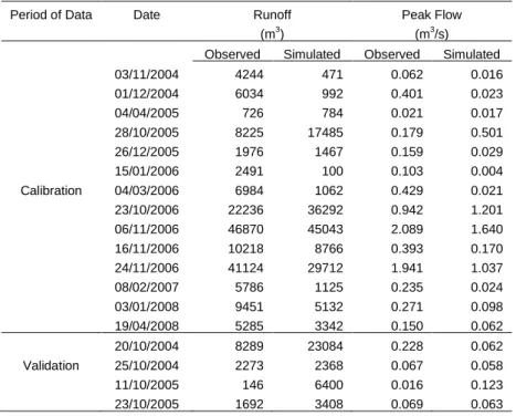
In this study, calibration was performed manually to select the parameter values so that the model closely simulates runoff and peak runoff rate (Mohammed et al., 2004). The calibration and validation of AnnAGNPS used data from the climate station available and it was performed through selection of individual significant and well identified peak runoff events at the daily scale. In these events, the baseflow is relatively smaller than the superficial and sub-surface flows. Studies indicated that baseflow separation analysis in some watersheds indicated low value (weighted average) base flow of the total direct flow (Kyoung et al., 2005; Li et al., 2006). Between October 2004 and April 2008, 28 events were selected and were alternately grouped into calibration and validation (Table 6). The superficial runoff dominates the hydrological response of this basin during the most significant events.
Table 6 - Observed and simulated of runoff volume and peak flow from the events used to the calibration and validation, for the period in analysis.
Period of Data Date Runoff (m3)
Peak Flow (m3/s) Observed Simulated Observed Simulated
Calibration 03/11/2004 01/12/2004 04/04/2005 28/10/2005 26/12/2005 15/01/2006 04/03/2006 23/10/2006 06/11/2006 16/11/2006 24/11/2006 08/02/2007 03/01/2008 19/04/2008 4244 6034 726 8225 1976 2491 6984 22236 46870 10218 41124 5786 9451 5285 471 992 784 17485 1467 100 1062 36292 45043 8766 29712 1125 5132 3342 0.062 0.401 0.021 0.179 0.159 0.103 0.429 0.942 2.089 0.393 1.941 0.235 0.271 0.150 0.016 0.023 0.017 0.501 0.029 0.004 0.021 1.201 1.640 0.170 1.037 0.024 0.098 0.062 Validation 20/10/2004 25/10/2004 11/10/2005 23/10/2005 8289 2273 146 1692 23084 2368 6400 3408 0.228 0.067 0.016 0.069 0.062 0.058 0.123 0.063
31/10/2005 04/11/2005 20/11/2005 02/12/2005 27/12/2005 18/03/2006 23/03/2006 25/10/2006 03/11/2006 08/12/2006 7746 5809 5566 9981 4902 2936 6436 23183 45795 14904 9416 7700 2812 1576 1408 862 559 19402 44081 1595 0.187 0.163 0.126 0.253 0.037 0.082 0.331 0.502 2.545 0.713 0.323 0.244 0.051 0.031 0.026 0.018 0.012 0.707 1.571 0.031
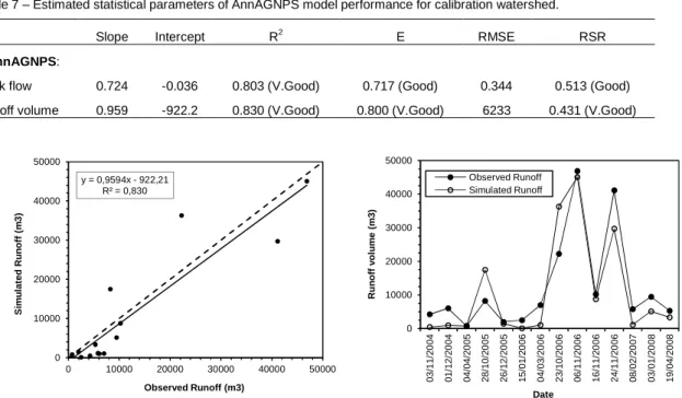
The calibration parameters for runoff volumes are listed in Table 7. Similar values were obtained at calibration efforts of AnnAGNPS model by other authors: Mohammed et al. (2004), 0.87 and 0.73 for R2 and E; Das et al. (2007), 0.79 for E; Taguas et al. (2009), 0.83 and 0.66 for R2 and E; and Licciardello et al. (2007), 0.84 for E. Our results indicate a good to very good agreement of simulated runoff by the AnnAGNPS model. This can be also visualized in Figure 2.
Table 7 – Estimated statistical parameters of AnnAGNPS model performance for calibration watershed.
Slope Intercept R2 E RMSE RSR
AnnAGNPS: Peak flow Runoff volume 0.724 0.959 -0.036 -922.2 0.803 (V.Good) 0.830 (V.Good) 0.717 (Good) 0.800 (V.Good) 0.344 6233 0.513 (Good) 0.431 (V.Good)
Figure 2 - Correlation between observed and simulated runoff on event scale in the calibration of the AnnAGNPS model.
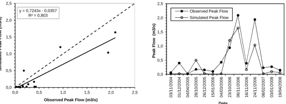
Regarding the peak flow, the calibration indicators obtained were 0.803, 0.717, and 0.513, for indicators R2, E and RSR, respectively. The ability of the model to simulate the peak values for each event can be considered in agreement with the calibration results from runoff values (Parajuli et al. 2009). The R2 value of 0.80 is similar to the value obtained by Mohammed et al. (2004) of 0.81, while the indicator E yielded 0.717 slightly higher than E value of 0.53 reported in the same study. Our findings also agree with findings from Licciardello et al., (2006) indicating that AnnAGNPS model overestimates the peak flow for the events with small amplitudes while underestimates the events with larger amplitude (Figure 3). y = 0,9594x - 922,21 R² = 0,830 0 10000 20000 30000 40000 50000 0 10000 20000 30000 40000 50000 S im u la te d R u n o ff ( m 3 ) Observed Runoff (m3) 0 10000 20000 30000 40000 50000 0 3 /1 1 /2 0 0 4 0 1 /1 2 /2 0 0 4 0 4 /0 4 /2 0 0 5 2 8 /1 0 /2 0 0 5 2 6 /1 2 /2 0 0 5 1 5 /0 1 /2 0 0 6 0 4 /0 3 /2 0 0 6 2 3 /1 0 /2 0 0 6 0 6 /1 1 /2 0 0 6 1 6 /1 1 /2 0 0 6 2 4 /1 1 /2 0 0 6 0 8 /0 2 /2 0 0 7 0 3 /0 1 /2 0 0 8 1 9 /0 4 /2 0 0 8 R u n o ff v o lu m e ( m 3 ) Date Observed Runoff Simulated Runoff
Figure 3 - Correlation between observed and simulated peak flow in the calibration of the AnnAGNPS model.
3.1.2. Irrigation season
The hydrologic behavior of the basin in irrigation season, under sprinkler irrigation systems mostly center-pivots, is much influenced by the proximity of the irrigation machines to the natural drainage network (Duarte, 2006). In a small irrigation basin, the hydrologic behavior is, consequently, much sensible by the irrigation practices, for example the irrigation scheduling and application depth; at this territorial scale, these irrigation parameters can present a considerable variability (Lorite et al., 2004).
By comparison of the observed and simulated runoff in full irrigation seasons (Table 8), we obtain statistical indicators higher than the same values verified for the rainfall season, although to be a data set lower than of the rainy season. Nevertheless, this is a good indication of the validity of AnnAGNPS model to simulate runoff in irrigation to larger periods of time, for example irrigation season.
Table 8 - Observed and simulated of runoff volume used in calibration for five irrigation season. Period of Data Date Runoff
(m3) Observed Simulated Irrigation Season 2004 2005 2006 2007 2008 65208 10396 2560 0 51466 47997 2196 5801 2767 66575
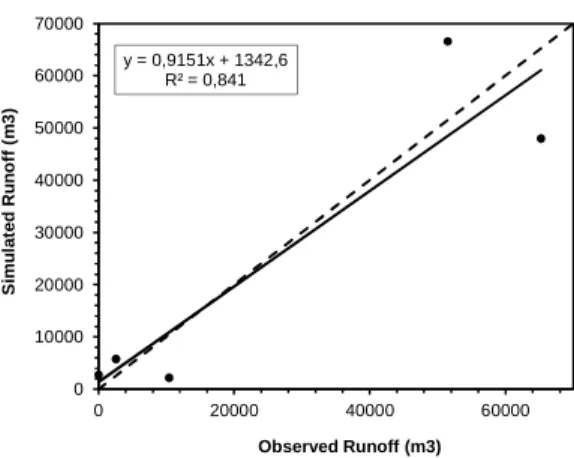
The values of statistical parameters obtained in the calibration, were the following: 0.841, 0.833 and 0.218, for R2, E and RSR, respectively (Table 10). These values make up a good or excellent capacity of AnnAGNPS model to simulate the irrigation return flows, at season time scale, as we can also observe in the Figure 4.
Table 9 – Estimated statistical parameters of AnnAGNPS model performance for calibration watershed (irrigation season).
Slope Intercept R2 E RMSE RSR
AnnAGNPS:
Runoff volume 0.915 1342.6 0,841 (V.Good) 0.833 (V.Good) 6600 0.218 (Excellent)
y = 0,7243x - 0,0357 R² = 0,803 0,0 0,5 1,0 1,5 2,0 2,5 0,0 0,5 1,0 1,5 2,0 2,5 S im u la te d P e a k F lo w ( m 3 /s )
Observed Peak Flow (m3/s)
0,0 0,5 1,0 1,5 2,0 2,5 0 3 /1 1 /2 0 0 4 0 1 /1 2 /2 0 0 4 0 4 /0 4 /2 0 0 5 2 8 /1 0 /2 0 0 5 2 6 /1 2 /2 0 0 5 1 5 /0 1 /2 0 0 6 0 4 /0 3 /2 0 0 6 2 3 /1 0 /2 0 0 6 0 6 /1 1 /2 0 0 6 1 6 /1 1 /2 0 0 6 2 4 /1 1 /2 0 0 6 0 8 /0 2 /2 0 0 7 0 3 /0 1 /2 0 0 8 1 9 /0 4 /2 0 0 8 P e a k F lo w (m 3 /s ) Date
Observed Peak Flow Simulated Peak Flow
Figure 4 - Correlation between observed and simulated runoff on season scale in the calibration of the AnnAGNPS model (irrigation season).
3.2. Validation of AnnAGNPS model
Some of calibration studies of hydrologic models, use data set for a continuous time period for calibration, and other data set for validation (Kliment et al., 2008; Poliakov et al., 2007). Given the randomness climate, especially in Mediterranean climate, we can have systematically low values in one of the continuous periods of time, and systematically high values in the other of the continuous periods of time. To prevent this situation, we were randomly selecting the values to the data set used in calibration and used in the validation. The data analysis in the Tables 10 and 7, allow concluding the better results obtained in the calibration than in the validation, but conforming the validation as good. The values are for the runoff volume, 0.721, 0.679 and 0.546, respectively for the statistical parameters R2, E and RSR. Das et al. (2007) in a similar study obtained an E value very similar (0.690); in the other hand, Mohammed et al. (2004) and León et al. (2004), in their studies achieved better E values (0.860 and 0.810, respectively).
Table 10 – Estimated statistical parameters of AnnAGNPS model performance for validation watershed.
Slope Intercept R2 E RMSE RSR
AnnAGNPS: Peak flow Runoff volume 0.574 0.878 0.058 148.6 0.742 (Good) 0.721 (Good) 0.676 (Good) 0.679 (Good) 0.358 6497 0.548 (Good) 0.546 (Good)
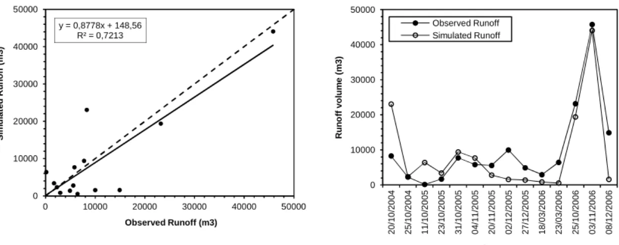
We can note, from observation the Figure 5, a higher dispersion of the observed and simulated data, than in the Figure 2 relating to calibration.
We can observed at Figure 5, as others authors have noted, at the beginning of the wet season runoff was generated by the AnnAGNPS but not observed in the same magnitude; this may depend on a defective model update of the antecedent moisture conditions for each rainfall event in those periods (Licciardello et al., 2006). y = 0,9151x + 1342,6 R² = 0,841 0 10000 20000 30000 40000 50000 60000 70000 0 20000 40000 60000 S im u la te d R u n o ff ( m 3 ) Observed Runoff (m3)
Figure 5 - Correlation between observed and simulated runoff on event scale in the validation of the AnnAGNPS model.
Respects to the peak flow validation, the values of statistical parameters are 0.742, 0.676 and 0.548, to R2, E and RSR, respectively. These values, except the RSR value, are slightly lower than the values obtained to the calibration, not calling into question the performance of AnnAGNPS model to predict the peak flow in isolated events. León et al. (2004) and Mohammed et al. (2004) calculated very similar values for the E parameter, 0.650 and 0.690, respectively. A lower performance was obtained by Nigussie and Fekadu (2003) in a small basin, where the E value was 0.340. Similarly as others authors (Shrestha et al., 2006; Haregewyen and Yohannes, 2003; Babel et al., 2004), we achieved in our study the tendency to the AnnAGNPS model overestimate the peak flow in the big events.
Observing the Figure 6, we can find a reasonable adherence between observed and simulated peak flow values.
Figure 6 - Correlation between observed and simulated peak flow on event scale in the validation of the AnnAGNPS model.
The results obtained in calibration and validation of the AnnAGNPS model, confirm a good or very good performance to simulate the peak flow and runoff volume at daily or event scale, as others authors have concluded in their studies (Taguas et al., 2009; Licciardello et al., 2006; Bhuyan et al., 2003). In the other hand, also the Curve Number methodology (USDA-SCS, 1986), show an adequate capacity to predict the runoff volume in experimental conditions, after well calibrated. However, Yuan et al. (2001; 2005) in AnnAGNPS applications to the small Mississippi watershed better results were achieved for monthly and annual runoff volumes with respect to the corresponding event scale estimations.
y = 0,8778x + 148,56 R² = 0,7213 0 10000 20000 30000 40000 50000 0 10000 20000 30000 40000 50000 S im u la te d R u n o ff ( m 3 ) Observed Runoff (m3) 0 10000 20000 30000 40000 50000 2 0 /1 0 /2 0 0 4 2 5 /1 0 /2 0 0 4 1 1 /1 0 /2 0 0 5 2 3 /1 0 /2 0 0 5 3 1 /1 0 /2 0 0 5 0 4 /1 1 /2 0 0 5 2 0 /1 1 /2 0 0 5 0 2 /1 2 /2 0 0 5 2 7 /1 2 /2 0 0 5 1 8 /0 3 /2 0 0 6 2 3 /0 3 /2 0 0 6 2 5 /1 0 /2 0 0 6 0 3 /1 1 /2 0 0 6 0 8 /1 2 /2 0 0 6 R u n o ff v o lu m e ( m 3 ) Date Observed Runoff Simulated Runoff y = 0,5738x + 0,0577 R² = 0,742 0,0 0,5 1,0 1,5 2,0 2,5 3,0 0,0 0,5 1,0 1,5 2,0 2,5 3,0 S im u la re d P e a k F lo w ( m 3 /s )
Observed Peak Flow (m3/s)
0,0 0,5 1,0 1,5 2,0 2,5 3,0 2 0 /1 0 /2 0 0 4 2 5 /1 0 /2 0 0 4 1 1 /1 0 /2 0 0 5 2 3 /1 0 /2 0 0 5 3 1 /1 0 /2 0 0 5 0 4 /1 1 /2 0 0 5 2 0 /1 1 /2 0 0 5 0 2 /1 2 /2 0 0 5 2 7 /1 2 /2 0 0 5 1 8 /0 3 /2 0 0 6 2 3 /0 3 /2 0 0 6 2 5 /1 0 /2 0 0 6 0 3 /1 1 /2 0 0 6 0 8 /1 2 /2 0 0 6 P e a k F lo w ( m 3 /s ) Date
Observed Peak Flow Simulated Peak Flow
Conclusions
After this study about a very important question, that is the selection and calibration a hydrologic model that simulates the non point source pollution originated by agriculture, more dangerous in irrigation agriculture, it´s possible to extract some conclusions reported bellow.
In the studies where the hydrologic aspects are very important, as the studies of non point source pollution at watershed scale, it come decisive the existence of good topographic information to made a DEM with proper vertical resolution, related with the study area. Usually, in the small basins, like our study basin, the hydrologic behavior is conditioned by the superficial runoff, namely when exist an impermeable soil layer.
The model AnnAGNPS appears to be a suitable tool for predicting non-point pollution due to some biogeochemical fluxes in irrigated agricultural watersheds. The experience on applying AnnAGNPS makes us think that the principles that support the model keep balance between complexity and applicability. Runoff and peak flow could be simulated in the study watershed reasonably well. Likely, a calibration of the parameters of the runoff sub-model would improve the performance of the model, but its inability to simulate base flow is a limitation inherent in the model.
Although the calibration of the AnnAGNPS model is based on only five irrigation seasons, the obtained results are a good indication of the validity of AnnAGNPS model to simulate runoff in irrigation to larger periods of time, for example irrigation season.
Except for the soil use oak/grass, the Curve Number values of all soil use goes to the extremes values of the interval range; these are the results verified with the methodology applied in this calibration. In future development of this study, is our intension use a methodology more accurate, like PEST algorithm, to confirm this tendency.
References
Arnold, J.G., R. Srinivasan, R. S. Muttiah, J. R. Williams. 1998. Large area hydrologic modeling and assessment, Part I: Model development. J. Am. Water Resour. Assoc. 34 (1), 73–89.
ASAE. 2005. ASAE Standards 2005. American Society of Agricultural Engineers, ASAE, St. Joseph, MI. Babel, M.S., M.N. Najim, R. Loof. 2004. Assessment of the AGNPS model for a watershed in tropical
environment. Journal of Environmental Engineering 130 (9), 1032e1041.
Baginska, B., W. Milne-Home, P. S. Cornish. 2003. Modelling nutrient transport in Currency Creek, NSW with AnnAGNPS and PEST. Environmental Modelling and Software 18 (8-9), 801e808.
Berry, J. K., J. A. Delgado, R. Khosla, F. J. Pierce. 2003. Precision conservation for environmental
sustainability. Journal of Soil and Water Conservation, Volume 58, Number 6, 332-339.
Bos, M. G., J.A. Replogle, A. J. Clemmens. 1991. Flow measuring flumes for open channel systems. American Society of Agricultural Engineers, St. Joseph, MI.
Bosch, D.D., R. Bingner, F.G. Theurer, G. Felton, I. Chaubey. 1998. Evaluation of the AnnAGNPS water quality model. ASAE Report No. 98- 2195, St. Joseph, MI.
Bhuyan, S.J., K.R. Mankin, J.K. Koelliker. 2003. Watershed-scale AMC selection on for hydrologic modelling. Transactions of the ASAE 46(2): 303–310.
Chaplot, V. 2005. Impact of DEM mesh size and soil map scale on SWAT runoff, sediment, and NO3–N loads predictions. Journal of Hydrology 312 (2005) 207–222.
Chung, S.W., P. W. Gassman, L. A. Kramer, J. R. Williams, R. Gu. 1999. Validation of EPIC for two watersheds in Southwest Iowa. J. Environ. Qual. 28 (3), 971–979.
Cohen, J. 2003. Applied Multiple Regresision – Correlation Analysis for the Behavioural Sciencies. Lawrence Erlbaum Associates: Malwah, NJ; 28.
Cronshey, R. G., F. G. Theurer. 1998. AnnAGNPS-Non Point Pollutant Loading Model. In Proceedings First Federal Interagency Hydrologic Modelling Conference, 19-23 April 1998, Las Vegas, NV.
Das, S., R. P. Rudra, B. Gharabaghi, P. K. Goel, A. Singh, I. Ahmed. 2007. Comparing the Performance of SWAT and AnnAGNPS Model in a Watershed in Ontario. Watershed Management to Meet Water Quality Standards and TMDLS (Total Maximum Daily Load) Proceedings. ASABE Publication number: 701P0207. ASABE, St. Joseph, MI.
Davis, D. M., P. H. Gowda, D. J. Mulla, G. W. Randall. 2000. Modeling nitrate leaching in response to nitrogen fertilizer rate and tile drain depth or spacing for southern Minnesota. USA J. Environ. Qual. 29 (5), 1568–1581.
Duarte, A. C. 2006. Contaminación difusa originada por la actividad agrícola de riego, a la escala de la
cuenca hidrográfica. Ph.D Thesis, University of Córdoba, Spain.
Duarte, A. C., F. J. Afonso, L. Mateos, E. Fereres. 2005. Resolution influence of the Digital Elevation
Model in the topographic configuration of the watershed. Water Resources, Journal of Water
Resources Portuguese Association, Vol.27 Nº1, 7-14.
FAO. 1998. World Reference Base for Soil Resources. FAO World Soil Resources Report 84. Food and Agriculture Organization of the United Nations, Rome.
FitzHugh, T. W., D. S. Mackay. 2000. Impacts of input parameter spatial aggregation on an agricultural nonpoint source pollution model. Journal of Hydrology 236, 35–53.
Garbrecht, J., W. Martz. 1995. Advances in automated landscape analysis. In: Proceedings of the First
International Conference on Water resources Engineering, Espey, W. H., P. G. Combs, Eds.,
American Society of Engineers, San Antonio, Texas, August 14-18, 1995, Vol.1, pp. 844-848.
Garbrecht, J., L. W. Martz. 1999. TOPAGNPS, An Automated Digital Landscape Analysis Tool for
Topographic Evaluation, Drainage Identification Watershed Segmentation and Subcatchment Parameterization for AGNPS 2001 Watershed Modelling Technology. Agricultural Research Service:
Washington, DC.
Grunwald, S., L. D. Norton. 2000. Calibration and validation of a non-point source pollution model. Agricultural Water Management 45 (1), 17-39.
Gumbel, E. J. 1958. Statistics of extremes. Columbia University Press.
Haregeweyn, N., F. Yohannes. 2003. Testing and evaluation of the agricultural non-point source pollution model (AGNPS) on Augucho catchment, Western Hararghe, Ethiopia. Agric. Ecosyst. Environ. 99, 201–212.
He, C. 2003. Integration of geographic information systems and simulation model for watershed management. Environmental Modelling & Software 18 (2003) 809–813.
INAG. 2008. Boletim de precipitação anual – Estação do Ladoeiro-14N/02U. Serviço Nacional de
Informação de Recursos Hídricos (SNIRH), Retrieved January 25, 2008, from the World Wide Web: http://snirh.inag.pt/snirhwww.php?main_id=18item=4.3.
ISO. 2005. Standard ISO 10390:2005 – Soil Quality - Determination of pH. International Organization for Standardization,Genéve, Switzerland.
Kalin, L., R. S. Govindarajua, M. M. Hantush. 2003. Effect of geomorphologic resolution on modeling of runoff hydrograph and sedimentograph over small watersheds. Journal of Hydrology 276, 89–111. Kliment, Z., J. Kadlec, J. Langhammer. 2008. Evaluation of suspended load changes using AnnAGNPS
and SWAT semi-empirical erosion models. Catena 73 (2008) 286–299.
Krause, P., D. P. Boyle, F. Base. 2005. Comparison of different efficiency criteria for hydrological model
assessment. Advances in Geosciences, 5: 89-97.
Kyoung J. L., B. A. Engel, Z. Tang, J. Choi, K. S. Kim, S. Muthukrishnan, D. Tripathy. 2005. Automated Web GIS based Hydrograph Analysis Tool, WHAT. Journal of American Water Resources Association 41(6): 1407–1416.
Legates, D. R., G. J. McCabe. 1999. Evaluating the use of "goodness of fit" measures in hydrologic and
hydroclimatic model validation. Water Resources Research, 35: 233-241.
León, L. F., W. G. Booty, G. S. Bowen, D. C. Lamb. 2004. Validation of an agricultural non-point source
model in a watershed in Southern Ontario. Agricultural Water Management, 65: 59–75.
Li, X., L. Frees, D. S. Moore, S. Wang. 2006. Calibrating the AnnAGNPS model in the Red Rock Creek watershed. Unpublished report. Department of Geography, University of Kansas, Lawrence, KS. Licciardello, F., D. A. Zema, S. M. Zimbone, R. L. Bingner. 2007. Runoff and soil erosion evaluation by
AnnAGNPS model in a small Mediterranean watershed. Transactions of the ASABE 59(5): 1585– 1593.
Licciardello, F., E. Amore, M. A. Nearing, S. M. Zimbone. 2006. Runoff and erosion modelling by WEPP
in an experimental Mediterranean watershed. In Soil erosion and sediment redistribution in river
catchments: Measurement, Modelling and Management. P.N. Owens and A.J. Collins (Eds), CABI. Lorite, I. J., L. Mateos, E. Fereres. 2004. Evaluating irrigation performance in a Mediterranean
environment. II. Variability among crops and farmers. Irrigation Science (2004) 23: 85-92.
Merriam, J. L., J. Keller. 1978. Farm Irrigation System Evaluation: A Guide for Management. Utah State University, Logan.
Mohammed, H., F. Yohannes, G. Zeleke. 2004. Validation of agricultural non-point source (AGNPS) pollution model in Kori watershed, South Wollo, Ethiopia. International Journal of Applied Earth
Observation and Geoinformation 6 (2004) 97–109.
Moriasi, D. N., J. G. Arnold, M. W. Van Liew, R. L. Bingner, R. D. Harmel, T. L. Veith. 2007. Model evaluation guidelines for systematic quantification of accuracy in watershed simulations. Transactions
of the ASABE 50(3): 885–900.
Nash, J. E., J. V. Sutcliffe. 1970. River flow forecasting through conceptual models. Part 1. A discussion of principles. Journal of Hydrology 10, 282-290.
Nelson, D. W., L. E. Sommers. 1982. Total carbon, organic carbon, and organic matter. In Methods of
Soil Analysis: Chemical and Microbiological Properties (part 2 (9), 2nd edition), Page AL, Miller H,
Keeney DR (eds). Soil Science Society of America: Madison, WI; 539–577.
Nigussie, H., Y. Fekadu. 2003. Testing and Evaluation of Agricultural Non-Point Source Pollution Model (AGNPS) on Augucho catchment, Western Hararghie, Ethiopia. Agriculture, Ecosystems and Environment 99, 201–212.
Parajuli, P. B., N. O. Nelson, L. D. Frees, K. R. Mankin. 2009. Comparison of AnnAGNPS and SWAT model simulation results in USDA-CEAP agricultural watersheds in south-central Kansas. Hydrol.
Process. 23, 748–763.
Polyakov, V., A. Fares, D. Kubo, J. Jacobi, C. Smith. 2007. Evaluation of a non-point source pollution model, AnnAGNPS, in a tropical watershed. Environmental Modelling & Software 22 (2007) 1617-1627.
Rawls, W. J., D. L. Brakensiek. 1989. Estimation of soil and water retention and hydraulic properties. In:
Unsatured flow in hydrologic modelling theory and practice, H. J. Morel-Seytoux (Ed.) Klwer Academic
Publeshers, Beltsville, MD, 275-300.
Sahrawat, K. L., K. V. Padmaja, P. Pathak, S. P. Wani. 2005. Measurable biophysical indicators for impact assessment: changes in water availability and quality. In: Shiferaw, B., Freeman, H.A., Swinton, S.M. (Eds.), Natural Resource Management in Agriculture: Methods for Assessing Economic
and Environmental Impacts. CAB International, Wallingford, UK, pp. 75–96.
Sarangi, A., C.A. Cox, C.A. Madramootoo. 2007. Evaluation of the AnnAGNPS Model for prediction of runoff and sediment yields in St Lucia watersheds. Biosystems Engineering 97 ( 2007 ) 241 – 256. Shrestha, S., S. Babel Mukand, A. Das Gupta, F. Kasama. 2006. Evaluation of annualized agricultural
nonpoint source model for a watershed in the Siwalik Hills of Nepal. Environmental Modelling &
Software, 21: 961-975.
Taguas, E. V., J. L. Ayuso, A. Peña, Y. Yuan, R. Pérez. 2009. Evaluating and modelling the hydrological and erosive behaviour of an olive orchard microcatchment under no-tillage with bare soil in Spain.
Earth Surf. Process. Landforms, Vol. 34, 738–751.
Twomlow, S., D. Love, S. Walker. 2008. The nexus between integrated natural resources management and integrated water resources management in southern Africa. Physics and Chemistry of the Earth 33, 889–898.
USDA-SCS. 1982. Soil Survey Laboratory Methods and Procedures for Collecting Soil Samples, Soil Survey Report 1. USDA: Washington, DC.
USDA-NRCS. 1986. Urban Hydrology for Small Watersheds. Technical Release 55, United States Department of Agriculture- Natural Resources Conservation Service, Washington, D.C.
Wani, S. P., P. Pathak, L. S. Jangawad, H. Eswaran, P. Singh. 2003. Improved management of Vertisols in the semi-arid tropics for increased productivity and soil carbon sequestration. Soil Use and
Management 19, 217–222.
Wischmeier, W. H., D. D. Smith. 1978. Predicting rainfall erosion losses. Agricultural Handbook No. 537. USDA, Washington, DC.
Yuan, Y., R. Bingner, F. Theurer, R.A. Rebich, P.A. Moore. 2005. Phosphorous component in
AnnAGNPS. Transactions of the ASAE, Vol. 48(6): 2145-2154.
Yuan, Y., R. L. Bigner, R. A. Rebich. 2001. Evaluation of AnnAGNPS on Mississippi Delta MSEA watersheds. Transactions of the ASAE 44(5): 1673–1682.