Advances in Mechanical Engineering 2016, Vol. 8(3) 1–10
ÓThe Author(s) 2016 DOI: 10.1177/1687814016638300 aime.sagepub.com
Nonlinear dynamic analysis of nuclear
fuels considering thermo–elastic–
plastic–creep phenomena
Young-Doo Kwon
1, Bo-Kyoung Shim
2and Ji-Min Song
2Abstract
Recently, research on the behavior of nuclear fuel rods in accident situations was performed. The research conducted was very sophisticated and involved complex tasks related to thermal, elastic, plastic, and creep phenomena. Previously, a nonlinear iterative static analysis for the behavior of a nuclear fuel rod was performed taking into consideration the thermal, elastic, plastic, and creep effects. However, the analysis cannot be applied to an unstable situation such as a bul-ging phenomenon of a nuclear fuel rod when a loss of coolant accident occurs. In this study, a nonlinear iterative dynamic analysis is performed considering large strain and thermo-mechanical effects, and the results of this dynamic analysis were obtained. The analysis is similar to those of static analysis; however, it differs from the static analysis after loss of coolant accident because of the inertia term of the dynamic equation.
Keywords
Nuclear fuel rod, nonlinear dynamic problem, Newton–Raphson iteration method, loss of coolant accident, large strain plasticity
Date received: 4 November 2015; accepted: 14 February 2016
Academic Editor: Nao-Aki Noda
Introduction
Energy consumption of human beings is drastically increasing till date and will increase further more in the future. The fossil energy will cease to serve sooner or later, and the alternative energy is still far less than the necessity. As the importance of nuclear energy is expected to be increased more and more, the safe con-trol of a nuclear power system including more precise prediction of the accidental behavior of nuclear fuels is required because of the formidable situation that would be encountered in case of an accident, which might happen without warning. Recently, researches on the behavior of nuclear fuel rods in accidents are being per-formed; the research conducted are very sophisticated and involved complex task related to thermal, elastic, plastic, and creep phenomena. Moreover, the strain may not be small; thus, we need a large strain plasticity analysis.
Thermo–elastic–plastic–creep analysis was fully developed using an equivalent stress function algorithm for small strain problems.1Large strain plasticity anal-yses were studied for isotropic and anisotropic prob-lems.2,3 Thermo–elastic–plastic–creep analysis considering large strain plasticity has been applied to nuclear fuel in loss of coolant accident (LOCA) situa-tion.4 However, the quasi-static analysis could not
1School of Mechanical Engineering & IEDT, Kyungpook National
University, Daegu, Korea
2Graduate School of Mechanical Engineering, Kyungpook National
University, Daegu, Korea
Corresponding author:
Young-Doo Kwon, School of Mechanical Engineering & IEDT, Kyungpook National University, 80 Daehakro, Bukgu, Daegu 702-701, Korea. Email: [email protected]
handle the bulging phenomenon at the final stage of deformation.
The bulging phenomenon is a type of stability prob-lem, and neither the quasi-static approach nor the post-buckling approach can be used to deal with this phe-nomenon, as these approaches are not suitable for problems where properties depend upon time and tem-perature. The only appropriate approach is a dynamic analysis considering the thermo–elastic–plastic–creep effects. This dynamic analysis will be developed and applied to the LOCA situation to show the thermo-mechanical behavior of fuels at the final stage of defor-mation. The results will show the exact time when the nuclear fuel rods will fail in a LOCA situation after the bulging phenomenon, which is a critical factor in the design and recovery of nuclear power plants.
Finite element analysis of nuclear fuels
including the bulging phenomena
For the analysis of the bulging phenomenon of a nuclear fuel rod, the heat transfer equation and the dynamic equation of motion will be presented. However, when the inertia term is neglected, the dynamic equation may be reduced to an equilibrium equation.
Nonlinear transient heat transfer equation
For the thermo–elastic–plastic–creep analysis of a nuclear fuel rod, it is necessary to obtain time-dependent temperatures by solving the following well-known transient equation of heat transfer
k(T,xx+ T,yy) + QcrT =_ 0
q = fB onGf
q =h(TT‘) onGh ð1Þ
where T is the temperature, k is the coefficient of the thermal conductivity, ris the density, c is the specific heat,qis the heat flow rate, fBis the heat flux, andhis
the convective heat transfer coefficient. The partial dif-ferential equation of heat transfer (equation (1)) is expressed in other functional forms to be minimized as in equation (2).5
Consider Y = ð 1 2T T
∂kT∂QT +crTT_
dV
ð
fBT +hT‘T
1
2hT
2
dS
ð2Þ
where k is the conductivity matrix and T∂ is the tem-perature gradient. After we introduce the finite elements with proper shape functions and minimize the
functional parameters, the following finite element equation is derived
t+DtC(i)t+DtT_(i1)+ (tKK+tKC)DT(i)
=t+DtQ+t+DtQC(i1)t+DtQK(i1) ð
3Þ
t+DtT(i)=t+DtT(i1)
+DT(i) ð4Þ Superscriptiindicates the quantity of iterative statei at time t+Dt; therefore, t+DtC is the heat capacity
matrix at time t+Dt,t+DtT_ is the rate of temperature
at time t+Dt,tKK is the conductivity matrix, andtKC
is the convection matrix at timet.DTis the incremental nodal point temperature,t+DtQis the nodal point heat
input vector, t+DtQC is the nodal point heat
contribu-tion due to conveccontribu-tion, and t+DtQK is the equivalent
nodal point heat contribution. Accordingly, to solve the unknown nodal point temperaturet+Dt
T, the equi-librium iteration will be performed repeatedly until the difference of the right-hand terms of equation (3) is smaller than the convergence tolerance.
Iterative nonlinear equation of motion
After obtaining the temperature distributions of the fuel, the incremental equilibrium equation for the motion of the fuel can be solved to obtain the incremen-tal displacements. Generally, the method for analyzing nonlinear problems includes the total Lagrangian and updated Lagrangian formulation. The updated Lagrangian formulation, which calculates the state at time t+Dt referring to the configuration at time t, is the method for nonlinear problems using the principle of the virtual work and the Cauchy stress tensor.
The principle of virtual work at time t may be expressed as
tR=ð
0 V
t
0Sijdt0eijd 0 V = ð 0 V t
0Cijrs t0ers+t0hrs
dt0eijd 0 V + ð 0 V t 0Sijdhijd
0
V
ð5Þ
where Cijrs is the material property tensor of stress–
strain.
The relation between the external virtual work tR
and the external force vectortPis as follows6
tR=dtUT tP
=
ð
0 V
dtUT t0BL0TD BLtUd 0 V + ð 0 V
dtUT t0BNLT t0S t
0BNL tUd 0
V
Applying the quotient law in order to obtain the equivalent nodal forces from equation (6)
tP=ð
0 V
t
0BL0TDBLtUd 0 V + ð 0 V t
0BNLT t0S t
0BNLtUd 0
V=t0F
ð7Þ
where t
0F is the equivalent nodal force vector
corre-sponding to the internal stresses at timet. It is the equi-librium state whentP=t
0F.
Because it establishes the equilibrium state when the external force is equal to the equivalent nodal force at timet+Dt
t+DtP=t+Dt
0F ð8Þ
Equation (8) can be written in the increment form as
t+Dt
P=t+Dt
0F=t0F+0F ð9Þ
where0F is the incremental nodal force vector, which
can be obtained approximately from the tangent stiff-ness matrix as
0F’t0KDU ð10Þ
DUdenotes the increment of the nodal displacement vectort+DtU. Substituting equation (10) to equation (9)
t
0KDU=t
+Dt
Pt0F ð11Þ
is obtained, and because the inertia force is added to body force, in dynamic problems, equation (11) can be written as
t
0KDU=
t+DtP
t0FM t+DtU€
ð12Þ
whereM=Ð 0
V 0
rHTHd0
V andHis the shape function matrix. The stiffness matrix in equation (12) can be decomposed into t
0K=t0KL+t0KNL, where the latter
term of stiffness is known as geometric nonlinear stiff-ness with regard to large displacement, buckling, and instability behaviors
K=KL+KNL= ð
0V
(BL0+BL1)TD(BL0+BL1)d0V ð13Þ
As equations (11) and (12) are linearized equations, they have some errors in comparison to the exact solu-tions. Therefore, iteration is required to correct the errors. Equation (12) can be expressed with the equili-brium by the Newton–Raphson iteration and Newmark method as follows6
t+Dt 0K(i
1)DU(i)=t+DtP
t+DtF(i1)
M 4
(Dt)2
t+DtU(i1)
tU
D4 t
tU_
tU€
ð14Þ
Superscriptiindicates the quantity of iterative state i. In order to simplify the displacement, equation (14) can be written as equation (15)
t+Dt
0K(i
1)DU(i)=t+DtP
t+DtF(i1)
Mt+D0tU€
(i) ð15Þ
As an iterative equilibrium equation which combines the Newton–Raphson iteration method and the Newmark integration method is used in the numerical calculation, equation (14) analyzes the nonlinear dynamic problems in this article. Ignoring the mass term in equation (15), the nonlinear incremental equili-brium equation for the quasi-static motion of the fuel can be obtained.
Thermo–elastic–plastic–creep analysis
The deviatoric stress is computed from the deviatoric strain while regarding the plastic and creep strain1,4 adopting the same symbols in Kojic and Bathe1as
t+Dt
S=
t+DtE
1+t+Dtn t+Dt
e0t+DtePt+DteC
ð16Þ
The mean stress is computed from the mechanical mean strain as equation (17)
t+Dt
sm=
t+DtE
12t+Dt
n t+Dt
emt+
Dt eth
ð17Þ
wheret+DtSis the deviatoric stress tensor,t+Dte0 is the
deviatoric strain tensor,t+Dt
ep is the plastic strain
ten-sor,t+Dt
ecis the creep strain tensor,t+Dt
smis the mean stress,t+Dt
emis the mean strain,t+Dteth is the thermal
strain,t+Dt
E is the Young’s modulus andt+Dt
n is the Poisson’s ratio at timet+Dt.
If we split the plastic and creep stains att+Dtinto the terms at timetand incremental terms, equation (17) then becomes
t+Dt
S=
t+DtE
1+t+Dtn t+Dt
e00DepDec
ð18Þ
where
t+Dte00=t+Dte0teptec ð19Þ
wheretepandtecare the plastic and creep strain at the
start of the current time step.
Creep strain may be represented by various creep laws such as the power creep law or the exponential creep law. To confirm plastic stress based on the given displacement,t+Dt
u(i), it must satisfy one of the yield
criteria. Adopting the von Mises yield criterion
fy=t+
Dt
t+Dt
s=pffiffiffiffiffiffiffiffiffiffiffiffiffiffiffiffiffiffiffiffiffiffiffiffiffiffiffiffiffiffiffiffiffiffi1:5t+DtSt+DtS:
von Mises equivalent stress ð21Þ
t+Dtsy= yieldstress ð22Þ
We have to solve the equation to obtain the deviato-ric stress tensor. By applying following flow rules of plastic and creep deformations
Dep=Dlt+DtS ð23Þ Dec=DttgtS ð24Þ
t= (1a)t+a(t+Dt):relaxed time ð25Þ
whereais the relaxation parameter. We obtain
t+DtS= 1
t+Dt
aE+aDttg+Dl t+Dt(e00(1a)DttgtS)
ð26Þ
where
aE=
1+n
E ð27Þ
Taking the product of both sides of the equation, we obtain the following equation
fg=a 2t+Dts2
+btgc2tg2d2=0 ð28Þ
where a=t+Dt
aE+aDttg+Dl= (1=2G0), b=
3(1a)Dtt+Dte00tS, c= (1a)Dtts, and
d2
=1:5t+Dte00t+Dte00.
The function on the left side of equation (28) is known as the effective-stress function, and it has to sat-isfy the condition of zero. Because s is a function of the plastic strain, andDlis also a function of the plas-tic strain and yield stress; equation (28) must be solved simultaneously forsandDlusing a root finding algo-rithm. Both the Newton method and the bisection method were used to find the proper roots. The latter method is very reliable without being affected by the derivative of the function. For the assumed
t+Dts( =t+Dts
y), Dl was computed first and then
checked whether the equation is satisfied. If the equa-tion cannot be satisfied, then the usual root finding algorithm can be used to findt+Dt
s( =t+Dt
sy) andDl simultaneously such that the chosen type of yield criter-ion is satisfied. The tangent constitutive matrix CEPC
can be obtained using the perturbation method.1,7 Here, we propose a first stage constitutive modulus as
C00=t+Dt 1
aE+l+Dttg
=2G00 ð29Þ
whereC00 is approximately closer to the tangent modu-lus thanC0. We could determine fast convergence with C00thanC0in several examples.
Large strain (Hencky logarithmic) measure
For large strain analysis, some basic relations are required which are briefly introduced here.2,3,8–11 The deformation gradient is represented by
t
0X=
∂tx
∂0x= tJT(0
J1)T ð30Þ
where J is the transformation between the Cartesian coordinate and natural coordinate systems. It can be decomposed into rotation tensor t
0R and right stretch
tensort 0U
t
0X=t0Rt0U ð31Þ
The right Cauchy–Green gradients are expressed using the deformation gradient
t
0C=t0XT t0X ð32Þ
Solving the following equivalent problem
t
0Ct0P=t0L 2 t
0P ð33Þ
A diagonal matrixt
0Lof principal stretches and their
direction matrix is then obtained. The right stretch matrix is
t
oU=t0Pt0Lt0PT ð34Þ
Therefore, the rotation matrix is given by
t
oR=toXtoU 1
ð35Þ
Then, the Hencky logarithmic strain tensor is given by
t 0EH=
1 2 t 0P t 0H t 0P
T ð36Þ
where
t
0H= lnL
2
ð37Þ
The Green–Lagrange strain tensor can be repre-sented as
t 0EG=
1
2
t
0CI
ð38Þ
and the Almansi strain tensor as
t 0EA=
1
2 I
0 tC
The Hencky logarithmic strain tensor can also be written as
t
0EH= ln t0U=
1
2ln
t
0C ð40Þ
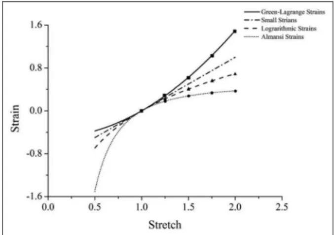
Using the equations above and comparing them (three kinds of marks) with theoretical equations (equa-tions (41)–(44)) in Figure 1 then
t 0e11=
1
2
t 0l
2
1
:GreenLagrange strain ð41Þ
te
11=t0l:small strain ð42Þ
t 0E
(H)
11 = ln t
0l:logarithmic strain ð43Þ
t teA11=
1
2 1
t 0l
2
:Almansi strain ð44Þ
Using the procedure of thermo–elastic–plastic–creep with logarithmic strain measure and additive decompo-sition of plastic strain, the developed Fortran program with additive decomposition method follows the proce-dures in Bathe and colleagues,2,8,9 except that plastic deformation gradient is not decomposed multiplica-tively as
XEA= t+Dt
0X t0Xp
1
ð45Þ
at the trial elastic state first, but considered additively as in equations (16) and (18). Therefore, continuation between later large strain procedure and former small strain procedure including creep deformation is not lost.
Verification of developed program
For the analysis of the bulging phenomenon of a nuclear fuel rod, analysis program is developed. The
developed FORTRAN program was tested with several cases.
Thermal analysis
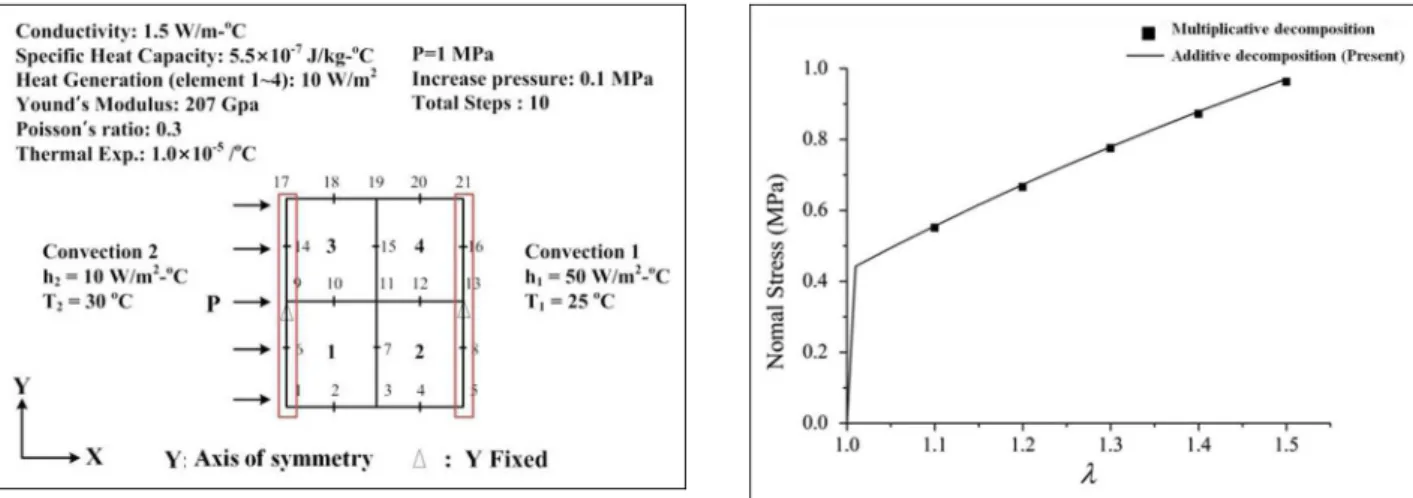
Thermal analysis4was performed using the present pro-gram and commercial package ADINA. The boundary conditions are shown in Figure 2.
Temperatures are analyzed and the results of three nodes are compared in Table 1 showing a good agreement.
Plasticity analysis
Plasticity analysis4 was performed using the present program and commercial package ADINA. The boundary conditions are shown in Figure 3.
The von Mises, radial, and hoop stresses are ana-lyzed for three cases of perfect, bilinear, and general plasticities. The initial value of the yield stress is 25 MPa, and the mechanical pressure load increases up to 9 MPa with 90 steps. As shown in Figure 4, the pres-ent program is proven to have a verified accuracy for the plasticity problems.
Creep analysis
Creep analysis was performed using the present pro-gram and commercial package ADINA.4 The bound-ary conditions are shown in Figure 5.
Figure 1. Strain–stretch relations for various strain measures.
Figure 2. Boundary condition for thermal analysis.
Table 1. Results of thermal analysis.
Temperature (°K)
Node 9 Node 11 Node 13
Present program 366.6 354.3 331.93
The von Mises, radial, and hoop stresses of the pres-ent program and ADINA are compared each other for creep problems as shown in Figure 6. The present pro-gram is reliable in the analysis of elasto-creep as well as in the thermal and plasticity analyses.
Large strain plasticity
For the case without creep deformation, the following example compares the two procedures of large strain
problems: additive decomposition (developed present program) and multiplicative decomposition.2The first one is uniaxial isochoric extension with the following conditions
Young’s modulus : E=200MPa Shear modulus : m=76:92MPa Bulk modulus : k=166:7MPa Poisson’s ratio : n=0:3 Yield stress : sy=0:75MPa
Hardening modulus : H=2MPa
An in-plane isochoric deformation with no rotation of the principal stretch directions, given by the defor-mation gradient
½X=
l 0 0
0 1=l 0
0 0 1
2
4
3
5 ð46Þ
wherel2[1, 1.5]. Figure 3. Boundary condition for plasticity analysis.
The results are compared in Figure 7 showing a good agreement.
The second example is shear deformation given by the deformation gradient
½X=
1 g 0 0 1 0 0 0 1
2
4
3
5 ð47Þ
whereg2[0, 0.5].
The result compared to the literature results (solid square) obtained by the multiplicative decomposition2 in Figure 8.
Behavior of nuclear fuel rods after LOCAs
considering the bulging effect
After a LOCA during the behavior of nuclear fuels, an unstable situation develops where the cladding stiffness becomes zero because of a local uncontrollable deformation.4 In this case, an analysis using the
post-buckling method applied to quasi-static problems is not a proper method for analyzing this transient problem because properties of the materials, which composed the nuclear fuel rods, are not constant. The material properties are considered functions of time and temperature. In order to analyze this type of phe-nomenon without divergence, the dynamic analysis method was adopted. Consequently, the bulging motion of the inflated nuclear fuel rods during a LOCA situation can be analyzed using the dynamic equation.
In the usual case of LOCA, the control rods are inserted into the fuel rods to shut down the reactor, and the power is reduced successfully. However, during events, such as the Fukushima accident, the control rods could not be inserted into the fuel rods because the insertion system, which is located at the lower part of the reactor, is malfunctioned. Therefore, it was assumed that the heat generation of the fuels was partly reduced. The material properties of the fuel components are the same as in the literature.12,13 Mesh generation of Figure 5. Boundary condition for creep analysis.
Figure 6. Results of creep analysis.
Figure 7. Normal stresssxalong stretchl.
the fuel rod was conducted using two-dimensional (2D) axisymmetric and quadrilateral eight-node elements, and the boundary conditions were applied as shown in Figure 9. The boundary conditions include the applica-tion of heat generaapplica-tion to the pellet as well as coolant pressure and convection heat transfer from the clad-ding to coolant. In addition, the gas pressure of the gap between the pellet and the cladding is also applied. The actual nuclear fuel rods are activated with mechanical and thermal properties shown in Table 2. In this article, the gas pressure of 34.5 MPa is applied to the analyses to assume the severe situation of the nuclear fuel rods. Figure 10 shows the temperature changes at the pellet center and cladding outer surface at steady-state condi-tions prior to 100 s.
The LOCA event was assumed to occur at 70 s resulting in a loss of coolant pressure and change in the ambient heat transfer coefficient from 7500 to 75 mJ/s mm2°K. In addition, the control rod is also malfunctioned. It was assumed that one of four condi-tions of heat generation (complete shutdown = 0%, 55%, 60% and full heat generation = 100%) was main-tained after LOCA. Temperature changes at the
cladding outer surface are shown in Figure 11. As expected, there were rapid changes in temperature at both the outer surface of the cladding because of the shutdown. It was detected that the outer surface of the Figure 9. (a) Solid nuclear fuel model and (b) boundary conditions.
Table 2. Mechanical and thermal properties.
Pellet Gap Cladding Coolant
TN – – 600°K –
Pressure (MPa) – 3.45 – 15.5
Density (mg/mm3) 1.0412e208 1.0412e208 6.5500e209 –
Heat generation (mJ/mm3s) 459 – – –
Convection (mJ/s mm2°K) – – 100 –
Specific heat (mJ/mg°K) 0.313889e+09 0.313889e+07 0.325896e+09 –
Thermal conductivity (mJ/s mm°K) 0.344808e+01 0.5 0.129064e+02 –
cladding shows a rapid increase in temperature and then the temperature increases slowly afterward at both 60% and 100% while temperature of the reactor con-tinued to decrease at complete shutdown after 70 s. After LOCA, there were sharp increases in temperature especially for full heat generation. The cladding with-stood the internal pressure load from the fuel rod. However, Young’s modulus and strength of the clad decreased since the cladding temperature beyond the steady-state temperature condition of 600°K. As a result, the fuel rod cannot resist the pressure load and deformation begins to occur, which causes larger stres-ses leading to fuel failure. This phenomenon is similar to buckling instability. The asterisk marks denote the divergence time at each heat generation in the quasi-static analysis of the fuel rods.
Figure 12 shows the radial displacements of the clad-ding outer surface during operation with considering
dynamic effects. The heat generation above 55% reac-tor power caused cladding instability, which then induced continuous expansion of the fuel rod ultimately leading to burst fuel rods. However, adopting the dynamic equation, the analyses was not been stopped due to the instability conditions. The variations of hoop stresses at the cladding surface are shown in Figure 13.
In the case of 60% and 100% heat generation after a LOCA, the behavior of the fuel rods could be analyzed using the dynamic equation without considering the cladding instability. This approach differed from Kim et al.4where the analyses do not consider the dynamic effects.
Conclusion
For the safe design and operation of a nuclear power plant, a precise thermo-mechanical analysis regarding the behavior of nuclear fuel rods in accidental situa-tions is required as well as the analysis for controlled operations. Thermo-mechanical analysis, including the thermal, elastic, plastic (large strain), and creep effect, on nuclear fuel comprehensively is rare. Moreover, the bulging phenomenon, which is the last stage of defor-mation followed by the bursting failure, cannot be ana-lyzed by a conventional quasi-static approach. We presented a nonlinear dynamic analysis of nuclear fuel rods considering the thermal, elastic, plastic (large strain), and creep effects for analyzing the bulging phe-nomenon in LOCA cases. It can be summarized as follows:
A comprehensive nonlinear iterative static analy-sis of nuclear fuel rods was made including the thermal, elastic, large strain plastic, and creep effects.
Figure 11. Temperatures at cladding outer surface with the LOCA at 70 s.
Figure 12. Radial displacements of cladding outer surface with the LOCA at 70 s.
A nonlinear iterative dynamic analysis procedure was formulated including the thermo-mechanical effects to handle the bulging phenomenon in LOCA situation.
The results of the dynamic analysis are very close to those of the static approach before the bul-ging. During the bulging phenomenon, dynamic results could be obtained while static analysis failed to proceed beyond the critical point.
Declaration of conflicting interests
The author(s) declared no potential conflicts of interest with respect to the research, authorship, and/or publication of this article.
Funding
The author(s) disclosed receipt of the following financial sup-port for the research, authorship, and/or publication of this article: This research was supported by the Basic Science Research Program through the National Research Foundation of Korea funded by the Ministry of Education (NRF-2012R1A1A2008903). The authors are partially sup-ported by the BK21 PLUS project of the Korean Research Foundation.
References
1. Kojic M and Bathe KJ. The ‘‘effective-stress-function’’ algorithm for thermo-elasto-plasticity and creep. Int J Numer Meth Eng1987; 24: 1509–1532.
2. Eterovic AL and Bathe K. A hyperelastic-based large strain elasto-plastic constitutive formulation with com-bined isotropic-kinematic hardening using the logarith-mic stress and strain measures. Int J Numer Meth Eng 1990; 30: 1099–1114.
3. Caminero MA´, Monta´ns FJ and Bathe K. Modeling large strain anisotropic elasto-plasticity with logarithmic strain and stress measures. Comput Struct 2011; 89: 826–843.
4. Kim JY, Kim DB, Cho HJ, et al. A critical heat genera-tion for safe nuclear fuels after a LOCA.Sci Tech Nucl Install2014; 2014: 150985.
5. Cook RD, Malkus DS, Plesha ME, et al.Concepts and applications of finite element analysis. New York: John Wiley & Sons, 2002.
6. Kim JU and Kwon YD. Nonlinear analysis of dynamics of beam with special boundary conditions.Trans Korean Soc Mech Eng1991; 15: 809–823.
7. Miehe C. Numerical computation of algorithmic (con-sistent) tangent moduli in large-strain computational inelasticity. Comput Method Appl M 1996; 134: 223–240.
8. Bathe KJ. Finite element procedures. Englewood Cliffs, NJ: Prentice Hall, 1996.
9. Kojic M and Bathe KJ. Inelastic analysis of solids and structures (Computational fluid and solid mechanics). Ber-lin: Springer, 2004.
10. Simo JC. A framework for finite strain elasto plasticity based on maximum plastic dissipation and the multiplica-tive decomposition: part I. Continuum formulation. Com-put Method Appl M1988; 66: 199–219.
11. Monta´ns FJ and Bathe KJ. On the stress integration in large strain elasto plasticity. Comput Fluid Solid Mech 2003; 2003: 494–497.
12. Kwon YD, Kwon SB, Song HJ, et al. Evaluation of nuclear fuel behaviors using finite element. Daejeon, South Korea: KAERI, 2010.